Research Article
Wavefront Reconstruction of Elevation Circular Synthetic
Aperture Radar Imagery Using a Cylindrical Green’s Function
Daniel Flores-Tapia,
1Gabriel Thomas,
2and Stephen Pistorius
1, 3, 41Division of Medical Physics, CancerCare Manitoba, Winnipeg, MB, Canada R3E 0V9
2Department of Electrical and Computer Engineering, University of Manitoba, Winnipeg, MB, Canada R3T 5V6 3Department of Radiology, University of Manitoba, Winnipeg, MB, Canada R3E 3P5
4Department of Physics and Astronomy, University of Manitoba, Winnipeg, MB, Canada R3T 2N2
Correspondence should be addressed to Daniel Flores-Tapia,[email protected]
Received 1 June 2009; Accepted 30 October 2009
Academic Editor: Laurent Ferro-Famil
Copyright © 2010 Daniel Flores-Tapia et al. This is an open access article distributed under the Creative Commons Attribution License, which permits unrestricted use, distribution, and reproduction in any medium, provided the original work is properly cited.
Elevation Circular Synthetic Aperture Radar (E-CSAR) is a novel radar modality used to form radar images from data sets acquired along a complete or even a segment of a cylindrical geometry above a given scan area. Due to the nonlinear nature of the target signatures on the E-CSAR data sets, the collected data must be focused. In this paper, a novel E-CSAR reconstruction algorithm is proposed. The proposed method uses a new formulation of the Green’s function of an E-CSAR scan geometry in which the phase components introduced by the scan geometry can be clearly identified and their effects can be effectively compensated. Additionally, theoretical aspects of the point spread function related to this new Green’s function were determined. The feasibility of the proposed technique was assessed using experimental data sets. The proposed method yielded spatially accurate images and exhibited an average execution time in the order of minutes.
1. Introduction and Motivation
Since its origins in 1951, Synthetic Aperture Radar (SAR) has been used for a wide variety of applications, from military reconnaissance to agricultural imaging to only name two examples [1]. Similarly to other radar imaging modalities, SAR techniques collect the reflections from an irradiated area and process them to create a reflectivity map from the scattering bodies present in the imaged region [2]. The SAR data acquisition process can be described as follows. A trajectory over the scan region is defined. Along this trajectory, an illuminating source radiates an ultra-wideband waveform and records the collected reflections from the objects inside the scan area. The recorded reflections are then processed to eliminate the distortions caused by the antenna, the shape of the irradiated waveform, and the motion of the moving platform [3–5]. Finally, the resulting reflectivity map can be visualized and interpreted.
The most commonly used scan geometries in SAR imaging scenarios are linear trajectories [3]. However, this
geometry [8]. This SAR modality is called Elevation Circular Synthetic Aperture Radar (E-CSAR) [3].
Similarly to other SAR scan geometries, E-CSAR data sets must be focused in order to be properly visualized and interpreted. Several reconstruction approaches have been proposed for this SAR modality, including Time Domain Correlation (TDC) techniques and Plane Wave Approxi-mation (PWA) methods. However, TDC techniques have execution times in the order of days or even weeks and PWA methods produce images with low focal quality, considerable spatial location errors and target smearing [9, 10]. An alternative approach is the use of waveform reconstruction techniques. These methods are based on performing a series of operations in the frequency domain that transfer the collected data from the spatiotemporal domain in which it was originally collected to the spatial domain where it will be displayed. It has been shown that wavefront reconstruc-tion techniques produce spatially accurate E-CSAR images [3].
Nevertheless, current E-CSAR wavefront reconstruction approaches still present limitations such as the execution times in the order of hours and altitude constraints [8, 11]. These considerations limit the widespread use of E-CSAR techniques in scenarios where the geometry of the scan region or target detection requirements suit the E-CSAR advantages, such as novel near field applications like breast microwave imaging [12], wood inspection [13], and low altitude SAR imaging scenarios [14]. In this paper, a novel E-CSAR wavefront reconstruction algorithm is proposed. Unlike current E-CSAR wavefront reconstruction approaches, the proposed method uses a novel formulation of Green’s function of the E-CSAR scan geometry that does not include a Hankel function and imposes no altitude restrictions on the inversion algorithm. The algorithm presented in this paper is an extension of the work presented by the authors in [15] for radar data sets acquired along cylindrical scan geometries. This paper is organized as follows. The E-CSAR signal model is explained inSection 2. InSection 3, the spectrum of Green’s function corresponding to the E-CSAR scan geometry is calculated. The proposed reconstruction method is described inSection 4. A theoreti-cal analysis of the point spread function of the E-CSAR imag-ing geometry, includimag-ing aspects such as the spatial samplimag-ing constraints and resolution, is done inSection 4. InSection 5, the feasibility of the proposed method is assessed using experimental data sets. Lastly, some concluding remarks are mentioned inSection 6.
2. Signal Model
Consider the scan geometry depicted inFigure 1. In E-CSAR scan scenarios, the data acquisition process is performed along a series of circular trajectories in the (x,y) plane defined along the z-axis. The antenna mainlobe is always pointing towards the center of a scan region with radiusRg.
The antenna radiation footprint is assumed to be constant over the scan region. A total ofTtargets are assumed to be present inside the scan area. The E-CSAR data acquisition process is performed as follows. At each scan location,
a waveform f(t) is irradiated and the responses from the targets present in the scan area are recorded. For the scan location at (R·cos(θ),R·sin(θ),z), the received signal can be expressed as
s(t,θ,z)=
T
p=1 σp(θ,z)
·f
t−2·
X+Y+zp−zc−z 2
/c
, (1)
where X denotes (xp−R·cos(θ))2, Y denotes (yp−
R·sin(θ))2, and z[0,zmax], c is the medium propa-gation speed, σi(θ,z) is the reflectivity of the pth target
when irradiated from (R·cos(θ),R·sin(θ),z), (xp,yp,zp)
is the location of thepth target, andzmin andzmax are the lower and upper spatial bounds of the scan trajectory along the azimuth direction. The frequency representation of the reflected signals from each target along thetdirection can be obtained by calculating its Fourier transform which yields the following expression:
Sp(ω,θ,z)=σp(θ,z)·F(ω)
·exp
−2k·
X+Y+zp−zc−z 2
, (2)
where k = ω/c which is known as the wavenumber and ω∈[ωmin,ωmax] andωmaxandωminare the maximum and minimum frequency components off(t), andp=1, 2,. . .,T. The exponential term in (3) is also known as the spherical phase function of the imaging system [3].
3. Wavefront Reconstruction
3.1. Green’s Function Spectrum Calculation. The collected data sets are a function of the signal travel time and the recording spatial location. Due to the different travel times of the target reflections and the shape of the scan geometry, the target responses exhibit nonlinear signatures when viewed on the (t,θ,z) domain. An example of this can be seen in Figure 2. This fact makes difficult to assess the locations and dimensions of the targets present in the scan area. If the collected data is directly mapped to a rectangular coordinate system, the target signatures appear at a shifted location and present a considerable augment on their dimensions. In order to properly visualize the target responses, the recorded data must be focused by transferring it from its original spatial temporal space to the spatial space related to the dimensions of the scan area. A common way of performing this process is to use the phase delay from the recorded reflections to determine its spatial location. This approach is known as wavefront reconstruction or holography [3,16, 17].
Let define the following distance function:
Lp(θ,z)=
R2+r2
p−2Rrpcos
ϕp−θ
+zp−zc−z 2
zc+zmax
zc+z
zc
Rg
x
y
z
R θ
(R,θ,z)
Figure1: E-CSAR scan geometry.
×10−9
2.3 2.4 2.5 2.6 2.7 2.8
Ti
m
e
(s
)
0 1 2 3 4 5 6
Angular location (rad)
Surface reflection
Target signatures
Figure2: Unprocessed experimental E-CSAR data corresponding
to 2 metal ovoids inside a PVC pipe.
x
y
α∗ β∗ R
(θn−ϕp)
(R,θn,zc)
Lp(θn,zc)
(rp,ϕp,zp)
Figure3: Angle geometry and nomenclature.
where
rp=
x2
p+y2p,
ϕp= ⎧ ⎪ ⎪ ⎪ ⎪ ⎪ ⎪ ⎪ ⎪ ⎪ ⎪ ⎪ ⎪ ⎪ ⎪ ⎪ ⎪ ⎪ ⎪ ⎪ ⎪ ⎨ ⎪ ⎪ ⎪ ⎪ ⎪ ⎪ ⎪ ⎪ ⎪ ⎪ ⎪ ⎪ ⎪ ⎪ ⎪ ⎪ ⎪ ⎪ ⎪ ⎪ ⎩
tan−1yp xp
ifxp>0, yp≥0,
tan−1yp xp
+ 2π ifxp>0, yp<0,
tan−1yp
xp +π ifxp<0,
π
2 ifxp=0, yp>0, 3π
2 ifxp=0, yp<0, 0 ifxp=0, yp=0.
(4)
The next step is to determine the Fourier transform of Sp(ω,θ,z) in the angular and elevation domains. This
operation is given by
Sp(ω,ε,kz)= zmax
0
2π
0 σp
(θ,z)·F(ω)
·exp−j·2k·Lp(θ,z) +εθ+kzz
dθ dz, (5)
whereε, andkz are the spatial frequency counterparts ofθ
andz respectively. To determine a closed form expression for (5), the stationary phase method will be used [17]. This technique determines the Asymptotic Behaviour (AB) of integrals containing a Phase Modulated (PM) function, as the value of the modulating terms tends to infinity. This approach determines the phase center of the PM term by analyzing the behaviour of its Instantaneous Frequency (IF). The AB is then determined by evaluating the PM function at the stationary point. The resulting expression is the frequency response of the imaging system. This technique has been used by several radar imaging reconstruction approaches to determine the frequency response of their corresponding imaging geometries [5,18–21].
×10−9 2.3 2.4 2.5 2.6 2.7 2.8
Ti
m
e
(s
)
0 1 2 3 4 5 6
Angular location (rad) Space definition
kux=krcos(θn)
kuy=krsin(θn)
Mapping from (kr,θn,kz)
to (kux,kuy,kz)
Interpolation from (kux,kuy,kz)
to (kx,ky,kz)
3D inverse Fourier transform Interpolation
(4k2−k2
z) kr
Inverse Fourier transform in the
εdirection 3D Fourier
transform
s(tl,θn,zm) S(ω
,ε,k z)
U(ω,ε,kz)
U(kr,ε,kz)
U(kr,θn,kz)
U(kr,θn,kz)
i(xa,yb,zm)
l(kx,ky,kz)
l(kux,kuy,kz)
F+(ω)exp(−J
⎛ ⎝
(4k2−k2
z)R2−ε2
+εsin−1(ε/
(4k2−k2
z)R) +επ+kzzc
⎞ ⎠)
−6.86
0
6.86 6.86 −3.43
0 3.43 6.86 7.5
2.5
−2.5
−7.5
z
(cm)
x(cm)
y(cm)
Figure4: Block diagram of the proposed inversion approach.
Phantom
Antenna Motor
Motor
90
cms
30
cms
70 cm
(a) (b)
y-axis
x-axis
1 cm 1 cm (a)
z-axis
x-axis
1 cm 1 cm (b)
z-axis
y-axis
1 cm 1 cm (c)
Figure6: Physical setup for experiment 1. (a) (x,y) plane view, (b) (x,z) plane view, and (c) (y,z) plane view.
0.15
0.1 0.05 0
z
(m)
−0.102
−0.034
0.034 0.102
y
(m)
−0.102 −0.068 −0.034 0 0.034 0.068 0.102
x(m) (a)
0.15
0.1
0.05
0
−0.102 −0.068 −0.034 0 0.034 0.068 0.102
y(m)
z
(m)
0
−0.102
x(m)
(b)
Figure7: Experiment 1 reconstructed 3D image: (a) (x,z) plane
view, and (b) (y,z) plane view.
θ∗. To make this process easier to follow, the value of z∗ will be calculated first. The IF in the z direction is given by
∂2k·Lp(θ,z) +εθ+kzz
∂z
= 2k·
zp−zc−z
R2+r2
p−2Rrpcos
ϕp−θ
+zp−zc−z 2−kz.
(6)
The phase center along the z direction, z∗, is defined as follows:
2k·zp−zc−z
R2+r2
p−2Rrpcos
ϕp−θ
+zp−zc−z 2 −kz
z=z∗
=0.
(7)
By making the left side of (6) equal to zero, the following expression is produced:
zp−zc−z∗
R2+r2
p−2Rrpcos
ϕp−θ
+zp−zc−z∗ 2 =
kz
2k. (8)
Notice how the left side of (8) resembles a trigonometric relationship. Taking advantage of this fact, (8) can be rewritten as
tan
⎛ ⎜ ⎜ ⎝sin−1
⎛ ⎜ ⎜
⎝ zp−zc−z
∗
R2+r2
p−2Rrpcos
ϕp−θ
+A
⎞ ⎟ ⎟ ⎠ ⎞ ⎟ ⎟ ⎠
=tan
sin−1
kz
2k
,
y-axis
x-axis
1 cm 1 cm (a)
z-axis
x-axis
1 cm 1 cm (b)
z-axis
y-axis
1 cm 1 cm (c)
Figure8: Physical setup for experiment 2. (a) (x,y) plane view, (b) (x,z) plane view, and (c) (y,z) plane view.
0.15 0.1
0.05 0
z
(m)
−0.102
−0.034
0.034 0.102
y
(m)
−0.102 −0.068 −0.034 0 0.034 0.068 0.102
y(m) (a)
0.15
0.1
0.05 0
−0.102 −0.068 −0.034 0 0.034 0.068 0.102
x(m)
z
(m)
0 0.102 y(m)
(b)
Figure9: Experiment 2 reconstructed 3D image: (a) (x,z) plane
view, and (b) (y,z) plane view.
whereAdenotes (zp−zc−z∗)2. By algebraically
manipu-lating (9), the next expression is obtained:
z∗=zp−zc−
kz
R2+r2
p−2Rrpcos
ϕp−θ
4k2−k2
z
. (10)
Next, the value ofz∗will be used to determine the AB of (5) along thezdirection. The resulting expression is
Sp(ω,ε,kz)
= 2π
0 σp(θ,kz)·F(ω)
·exp
−j·4k2−k2
z·Dp(θ,z) +εθ+kzzp−kzzc
dθ, (11)
where σp(θ,kz) is the spectrum amplitude component
in the (θ,kz) domain, ε and kz are the frequency
counterparts of θ and z, respectively, and Dp(θ,z) = R2+r2
p−2Rrpcos(ϕp−θ). Next, the asymptotic
behaviour in theθdirection will be calculated. The IF of the PM component of (11) in theθdirection is
∂−4k2−k2
z·Dp(θ,z) +εθ+kzzp−kzzc
∂θ
= −
4k2−k2
z
·R·rp·sin
ϕp−θ
R2+r2
p−2Rrpcos
ϕp−θ
−ε. (12)
The phase centerθ∗is defined as:
−
4k2−k2
z
·R·rp·sin
ϕp−θ
R2+r2
p−2Rrpcos
ϕp−θ −ε
θ=θ∗
=0. (13)
By algebraically manipulating (13), the following expression is obtained:
sinϕp−θ∗
R2+r2
p−2Rrpcos
ϕp−θ∗
= −ε
4k2−k2
z
·R·rp
.
y-axis
x-axis
1 cm 1 cm (a)
z-axis
x-axis
1 cm 1 cm (b)
z-axis
y-axis
1 cm 1 cm (c)
Figure10: Physical setup for experiment 2. (a) (x,y) plane view, (b) (x,z) plane view, and (c) (y,z) plane view.
0.15 0.1 0.05 0
z
(m)
−0.102
−0.034
0.034 0.102
y(m)
−0.102−0.068−0.034 0 0.034 0.068 0.102
x(m) (a)
0.15 0.1 0.05 0
0.102 0.068 0.034 0 −0.034−0.068−0.102
y(m)
z
(m)
0.102 0.034
−0.034
−0.102 x(m)
(b)
Figure11: Experiment 3 reconstructed 3D image: (a) (x,z) plane
view, and (b) (y,z) plane view.
By using the fact that the left side of (14) resembles a sine law relationship, an analytical solution can be obtained. As depicted in Figure 3, a triangle between the pth target, the antenna, and the center of the scan pattern is formed. Using basic trigonometry concepts, it can be shown thatθ∗=ϕp+
α∗+β∗−π. Therefore, the relationship between (ϕp−θ∗),
α∗andβ∗is given by
sinϕp−θ∗
R2+r2
p−2Rrpcos
ϕp−θ∗
=sin(α∗)
rp =
sinβ∗
R =
−ε
4k2−k2
z
·R·rp
. (15)
From (16), the values ofα∗andβ∗are
α∗= −sin−1
⎛
⎝ ε
4k2−k2
z
·R
⎞
⎠, (16)
β∗= −sin−1
⎛
⎝ ε
4k2−k2
z
·rp
⎞
⎠. (17)
Next, the AB of (5) is calculated by evaluating (11) atθ∗. The resulting expression is
Sp(ω,ε,kz)
=σp(ε,kz)·F(ω)
·exp
−j·4k2−k2
z
rp2−ε2+
4k2−k2
z
R2−ε2
+ε·sin−1
⎛
⎝ ε
4k2−k2
z
·R
⎞ ⎠
+ε·sin−1
⎛
⎝ ε
4k2−k2
z
·rp
⎞ ⎠
+ε·π+ε·ϕp+kzzp−kzzc
,
where σp(ε,kz) is the spectrum amplitude component in
the (ε,kz) frequency space. In the majority of the E-CSAR
scenarios,s(t,θ,z) is defined over an L×N ×M discrete space (tl,θn,zm), whereLis the number of time samples,Nis
the total scan locations in the circular scan pattern defined in the (x,y)-plane, M is the total number of scan planes along thez-axis, andl,n,andmdenote the sample indexes alongt,θ, andzscan trajectories in that order. Given that the Shannon-Nyquist theorem was satisfied the mathematical analysis shown in the last subsection holds true for the 3D discrete Fourier transform of s(tl,θn,zm), and S(ω,ε,kz), whereω,ε, andkzare the discrete counterparts ofω,ε, and
kz, respectively.
3.2. Image Reconstruction. In order to properly visualize the recorded reflections, the effect of the scan geometry must be compensated and the data must the migrated from the (t,θ,z) domain to the rectangular space (x,y,z) where it will be visualized and interpreted. The following steps can be used to form the 3D image,i(xa,yb,zm), whereaandbare
the sample indexes along thex- andy-axes, corresponding to the collected data sets(tl,θn,zm).
(1) Calculate the 3D FFT ofs(tl,θn,zm). The result of this
operation isS(ω,ε,kz).
(2) Next, the effects of the scan trajectory on the collected data are removed. The phase terms in (18) can be divided into two main types. The first one, denoted byB(ω,ε,kz), is the PM terms related to the target responses. These terms are a function of the target location, (rp,ϕp,zp). The second type
of spectral components,C(ω,ε,kz), is the PM terms related to the delays produced by the shape of the scan geometry. In order to eliminate the effects of the scan trajectory on the collected data, C(ω,ε,kz) must be removed from S(ω,ε,kz). This is achieved by performing the following operation:
Uω,ε,kz
=Sω,ε,kz
·Cω,ε,kz
+
, (19)
where C(ω,ε,kz)+ denotes the complex conjugate of C(ω,ε,kz) which is equal to
Cω,ε,kz
+
=F(ω)+
·exp
⎛ ⎝j·
⎛
⎝4k2−k2
z
R2−ε2
+ε·sin−1
⎛
⎝ ε
4k2−k2
z
·R
⎞
⎠+ε·π−kzzc ⎞ ⎠ ⎞ ⎠.
(20)
The resulting spectrum is given by
Uω,ε,kz
=
T
i=1 σi
ε,kz
·exp
⎛ ⎝−j·
⎛
⎝4k2−k2
z
r2
i −ε2+ε
·sin−1
⎛
⎝ ε
4k2−k2
z
·ri
⎞
⎠+ε·ϕi+kzzi ⎞ ⎠ ⎞ ⎠,
(21)
wherek=ω/c.
(3) The next step is to transfer the data inU(ω,ε,kz), from the (ω,ε,kz) frequency space to the (kx,ky,kz) spatial
frequency space, wherekx andky are the spatial frequency
counterparts of thexandyspatial domains. For this purpose, the auxiliary function kur(ω,kz) =
(4k2−k2
z ) will be
used. Due to the fact that bothkandkzare evenly sampled,
the differences between adjacent values within kur(ω,kz) vary across the grid in which the function is defined. As mentioned in [22], uneven sampled frequency spaces are unfit to be processed using FFT-based techniques. To generate a space without this issue, the functionkr(ω,kz) is defined, where the differences between the values present at adjacent samples are the same for all its domain grid,Δkr =
π/R. We will denote the set of values present inkr(ω,kz) by the (kr,kz) frequency space. To produce a spectrum suitable to be processed using FFT techniques, the data present in each (ω,kz) plane in U(ω,ε,kz), is interpolated into the frequency values specified in the (kr,kz) space. This operation is performed for each plane in theεdirection. The outcome of this process will be referred asU(kr,ε,kz). This process is also known as Stolt‘s interpolation [19–21].
(4) The inverse FFT of the focused data is computed on theεdirection, resulting in a representation of the collected data in the (kr,θn,kz) domain. We will refer to the resulting spectrum byU(kr,θn,kz).
(5) At this point, a new frequency space, denoted by (kux,kuy,kz) is generated, where
kux=kr·cos(θn),
kuy=kr·sin(θn).
(22)
This mapping is performed for the (kr,θn) plane
correspond-ing to eachkzvalue.
(6) Next, we can mapU(kr,θn,kz) into (kux,kuy,kz) using the following function:
Ikux,kuy,kz
=Ukr,θn,kz
∀(u,v)∈ρ,ϕ, (23)
where the corresponding (kux,kuy) for each (kr,θn) point is
given by (22).
resulting in a nonuniformly sampled frequency space. In order to obtain an evenly sampled spectrum, a new discrete frequency space, denoted by (kx,ky,kz), is defined. In
this space the separation between samples in each (kx,ky)
plane is Δky = Δkx = π/R. Next, the evenly sampled
spectrumI(kx,ky,kz) is generated by interpolating the data
contained inI(kux,kuy,kz) into the frequency values specified
in the (kx,ky,kz) space.
(8) Finally, in order to visualize the reconstructed data in the spatial domain a 3D inverse FFT is applied toI(kx,ky,kz).
The result of this process is the 3D modeli(xa,yb,zm). A
flow diagram of the reconstruction process can be seen in Figure 4.
4. Point Spread Function Analysis
4.1. Preliminaries. The point spread function (psf) is an important analytical tool to assess the spatial constraints of a radar system. This mathematical expression provides a measure of the spatial resolvability of a particular scan geometry and waveform. Additionally, the psf is also used to determine the spatial sampling criteria needed to properly record and reconstruct radar data sets. In general, the point spread function of the pth target along a generic scan trajectorywis modeled as follows:
psfpΩw,p,w
=Ωw,psinc
Ω w,p·w
2π
, (24)
where Ωw,p is the support band of the collected responses
from thepth target along thewscan direction. The extension of Ωw,p is obtained by calculating the difference between
the maximum and minimum IF values along each scan trajectory [3]. From basic radar signal theory, it is well known that the support band corresponding to the fast time trajectorytis the same for all the targets in the scan area, or in other words,|Ωt,p| =B, whereBis the bandwidth of the
radiated waveform. The psf function of a radar signal in the fast time trajectory is given by
psfp(B,t)=4πB v sinc
B·t v
. (25)
The spatial resolution achieved by this psf is equal to
Δtp= v
2B. (26)
To properly define the psf for a multidimensional SAR system, the support bands along the slow time trajectories must be calculated. Thus, in the following discussion, the behaviour of the psf in theθandztrajectories is analyzed. The corresponding resolution values in both slow-time trajectories are calculated and the corresponding sampling requirements are determined.
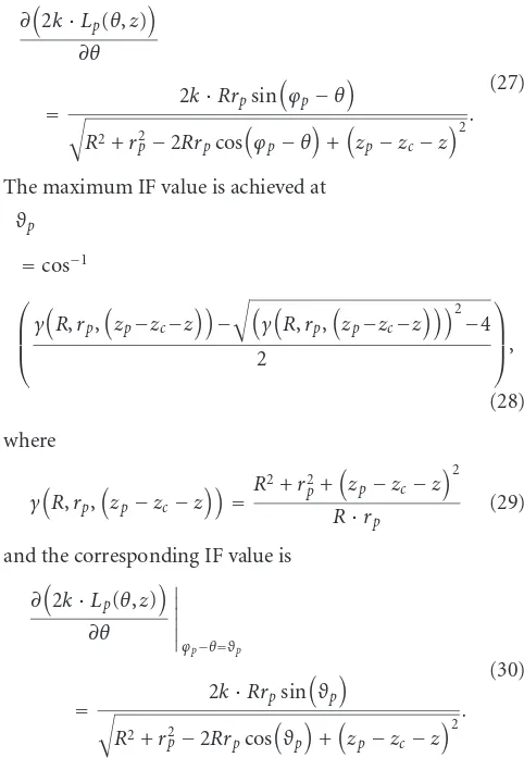
4.2. Angular Scan Trajectory. For the E-CSAR spf, the IF along theθscan direction is given by
∂2k·Lp(θ,z)
∂θ
= 2k·Rrpsin
ϕp−θ
R2+r2
p−2Rrpcos
ϕp−θ
+zp−zc−z 2.
(27)
The maximum IF value is achieved at ϑp
=cos−1
⎛ ⎜ ⎜ ⎝
γR,rp,
zp−zc−z
−γR,rp,
zp−zc−z 2 −4 2 ⎞ ⎟ ⎟ ⎠, (28) where
γR,rp,
zp−zc−z
= R
2+r2
p+
zp−zc−z 2
R·rp
(29)
and the corresponding IF value is
∂2k·Lp(θ,z)
∂θ
ϕ
p−θ=ϑp
= 2k·Rrpsin
ϑp
R2+r2
p−2Rrpcos
ϑp
+zp−zc−z 2.
(30)
Similarly, it can be shown that the minimum IF value with respect toθis achieved whenϕp−θ=2π−ϑp. The IF value
in this case is
∂2k·Lp(θ,z)
∂θ
ϕ
p−θ=2π−ϑp
= − 2k·Rrpsin
ϑp
R2+r2
p−2Rrpcos
ϑp
+zp−zc−z 2.
(31)
Therefore, the value ofΩθ,pis given by
Ωθ,p=
2k·Rrpsin
ϑp
R2+r2
p−2Rrpcos
ϑp
+ (zp−zc−z2)2
− −2k·Rrpsin
ϑp
R2+r2
p−2Rrpcos
ϑp
+ (zp−zc−z2)2
,
Ωθ,p=
4k·Rrpsin
ϑp
R2+r2
p−2Rrpcos
ϑp
+ (zp−zc−z2)2
.
Ωθ,pis not the same for all the targets in the scan area,
because it is a function of the target location and the scan plane. Nevertheless an accurate estimate of the psf mainlobe width can be calculated by using the center value of the domains ofk,rp, and (zp−z) [2]. For a set of fixedRand Bvalues, the average spatial resolution that can be achieved in this support band is given by
Δθrq,zq
=c
R2+rq/22−2Rrq/2cosρ+zq/22
4fc·R·
rq/2
sinρ ,
(33)
whererqis the radius of the scan area,zqis the length of the
scan geometry along thez-axis, fcis the center frequency of
the emitted signal, and
ρ=cos−1
⎛ ⎜ ⎜ ⎝
γR,rq/2,zq/2
−γR,rq/2,zq/2
2
−4
2
⎞ ⎟ ⎟ ⎠.
(34)
Finally, to avoid the presence of aliasing along theθscan direction in the collected data, the spacing between scan locations in this slow-time direction must be set in such a way that the Nyquist sampling criterion is satisfied. For this purpose, the maximum value thatΩθ,pcan achieve must be
determined, within the limits imposed by the scan trajectory. A simple way of determining this value is by substituting the upper bound values of the domains corresponding to thek, rp, and (zp−z) variables into the right side of (31). The
resulting expression is
∂2k·Lp(θ,z)
∂θ
k=k
m,rp=rq,(zp−zc−z)=zq,ϕp−θ=ϑ
= 2km·Rrqsin
ϑ
R2+r2
q−2Rrpcos
ϑ+z2
q
,
(35)
where
ϑ=cos−1
⎛ ⎜ ⎜ ⎝
γR,rq,zq
−γR,rq,zq
2
−4
2
⎞ ⎟ ⎟ ⎠, (36)
andkm is the maximum wavenumber value present in the
emitted signal. Therefore, the angular separation between adjacent scan locations along theθscan direction,δθ, must satisfy the following criterion:
δθ≤ c
R2+r2
q−2Rrqcos
ϑ+z2
q
4fm·R·rqsin
ϑ , (37)
where fmis the minimum wavelength present in the radiated
signal.
4.3. Azimuth Scan Trajectory. The IF of the E-CSAR psf with respect tozis
∂2k·Lp(θ,z)
∂z
= 2k·
zp−zc−z
R2+r2
p−2Rrpcos
ϕp−θ
+zp−zc−z 2.
(38)
And the size of the support band is
Ωz,p=
2k·zp−zc+zq/2
R2+r2
p−2Rrpcos
ϕp−θ
+zp−zc+zq/2 2
− 2k·
zp−zc−zq/2
R2+r2
p−2Rrpcos
ϕp−θ
+zp−zc−zq/2 2.
(39)
The support band for this slow time trajectory Ωz,p is
also a function of the target location and the scan angle. In this case we can also use the center values of the domains corresponding tok,rp, (zp−zc−z), and (ϕp−θ) to define
an average value for the support band. Following a similar approach to the one used for (35), the average psf mainlobe size in thezdirection (with fixedRandB) values is equal to
Δzrq,zq
=c
R2+r
q/2 2
+zq/2 2
4fc·R·zq .
(40)
Finally, in order to satisfy the Nyquist criterion in thezscan trajectory, the spacing between scan planes,δz, must satisfy the following condition:
δz≤c
R2+r2
q+z2q
4fm·R·zq .
(41)
5. Results
Table1: Permittivity values of the materials used in the phantom structure and support base.
Material Permittivity value (6 GHz)
PVC 3
Air 1
Maple wood 1.55–1.7
Synthetic foam 1.05
locations. A SFCW waveform with a bandwidth of 11 GHz (1–12 GHz) was used in all the experiments. The system was characterized by recording the reflections of a steel sphere inside an anechoic chamber. The reference signal was subtracted from the experimental data in order to eliminate distortions introduced by the system components. The data acquisition setup was surrounded by electromagnetic wave absorbing material to reduce undesirable reflections from the surrounding environment. The data was reconstructed using a 2.6 GHz dual processor PC with 3 GB RAM.
The phantom used in all the experiments consists of a Polyvinyl Chloride (PVC) pipe filled with synthetic foam disks. The PVC pipe was used as a support structure and has an inner diameter of 10 cm and a height of 90 cm. Aluminum ovoids were used as targets. The ovoids have a 1.2 cm diameter and a 3 cm height. The dielectric permittivity values of the materials used in the support base and the phantom structure are shown inTable 1. A diagram and a photograph of the data acquisition setup can be seen in Figures5(a)and 5(b), respectively.
The data acquisition process was performed by rotating the phantom at 5◦ intervals for a total of 72 positions. Along the z-axis, the data was acquired at 15 scan planes with a separation of 1 cm. The value of zc in all the
experiments was 10 cm. In order to allow the beamwidth to illuminate the entire phantom and reduce undesirable interferences of antenna early time artifacts, the distance between the antenna and the center of the phantom was set to 70 cm. A zero padding factor of 2 was used to improve the visualization of the reconstructed images. In the following discussion, the center of the phantom will be denoted as the origin, and the displayed images show the normalized energy of the reconstructed data. The sampling along the slow time scan trajectories,qandz, was done according to the criteria set in the previous section.
The data collected from three experimental setups was used to determine the feasibility of the proposed approach and assess its performance. In all the experiments, the sepa-ration between the targets was at least equal to twice the value of the spatial resolution along the fast time scan trajectory (1.36 cm). In the first experiment, a single ovoid positioned at (0, 2, 5.5) cm was used. A diagram of the experimental setup can be seen inFigure 6. The reconstructed 3D model is shown inFigure 7. In order to have a better visualization of the target signatures, the PVC pipe reflections were removed using the method proposed by the authors in [23]. In the second experiment, two targets were positioned at (0,−2.5,9) cm and (2.5,0,6) cm. The experimental setup can be seen in Figure 8. The reconstructed image viewed
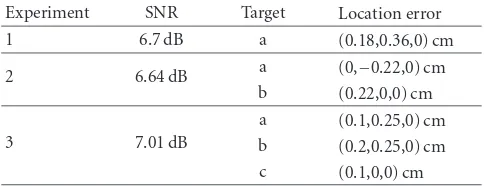
Table2: Location errors and SNR values obtained in each image.
Experiment SNR Target Location error
1 6.7 dB a (0.18,0.36,0) cm
2 6.64 dB a (0,−0.22,0) cm
b (0.22,0,0) cm
3 7.01 dB
a (0.1,0.25,0) cm
b (0.2,0.25,0) cm
c (0.1,0,0) cm
from an (x,z) plane perspective is shown in Figure 9(a). The corresponding (y,z) plane perspective view is shown in Figure 9(b). The third experimental setup is shown in Figure 10. In this scan scenario, 3 targets were positioned at (−2,2,6) cm, (2.5,2,8.5) cm, and (0,−2.5,12) cm. The reconstructed 3D model viewed from anx-axis perspective is shown inFigure 11(a). The correspondingy-axis perspective view is shown inFigure 11(b).
To quantitatively assess the performance of the proposed method, the spatial errors of the reconstructed target signatures and the Signal-to-Noise Ratio (SNR) of each reconstructed image were calculated. The SNR of the 3D images was determined as follows:
SNRw=20·log10 ⎛ ⎝
T
q=1Γq,3 dB/T σw
⎞
⎠, (42)
where Γp,3 dB is the magnitude of the 3 dB point of the
pth target signature in the 3D model generated by the proposed algorithm and σw is the standard deviation of
the background noise. The locations errors of the target signatures and SNR of each reconstructed image are shown inTable 2. Finally, the computational cost of the proposed technique was evaluated. The simulated data sets were generated using the radar simulation tool proposed by the authors in [24]. The execution time of a set of 75 simulated sets was measured. The number of angular scan locations in each plane was 200, and the number of scan planes was set to 21. The order of complexity of the proposed algorithm was O(n·log(n)), where nis the number of data points. This resulted in an average execution time of 10 minutes and 10 seconds (30.5 seconds per plane) for a single data set on the PC used for data processing.
6. Conclusions
terms in the form of Hankel functions, making the proposed reconstruction method computationally efficient.
Theoretical aspects, such as the size of the psf and sampling constraints, were analyzed. In order to determine the experimental feasibility of the proposed method an experimental data acquisition system was assembled. The proposed methods produced spatial accurate imagery with acceptable SNR values at reasonable computational cost. Future research will be concentrated on two main aspects. First, the proposed techniques will be tested on experimental data sets collected from more complex phantoms in order to evaluate their feasibility on more realistic scenarios. Finally, another area of interest is the reduction of the computational cost of the proposed algorithms.
Acknowledgments
This research was supported by CancerCare Manitoba, Mathematics of Information Technology and Complex Sys-tems, The University of Manitoba, and the Natural Sciences and Engineering Research Council of Canada.
References
[1] G. Franceschetti, Synthetic Aperture Radar Processing, CRC Press, Boca Raton, Fla, USA, 1999.
[2] D. R. Wehner,High-Resolution Radar, Artech House, Nor-wood, Mass, USA, 2001.
[3] M. Soumekh,Synthetic Aperture Radar Signal Processing with MATLAB Algorithms, Wiley-Interscience, New York, NY, USA, 1999.
[4] J. Sok-Son, G. Thomas, and B. C. Flores,Range-Doppler Radar Imaging and Motion Compensation, Artech House, Norwood, Mass, USA, 2001.
[5] M. Soumekh, “A system model and inversion for synthetic aperture radar imaging,”IEEE Transactions of Image Process-ing, vol. 1, no. 1, pp. 64–76, 1992.
[6] M. L. Bryant, L. L. Gostin, and M. Soumekh, “3-D E-CSAR imaging of a T-72 tank and synthesis of its SAR reconstruc-tions,”IEEE Transactions on Aerospace and Electronic Systems, vol. 39, no. 1, pp. 211–227, 2003.
[7] B. Edde, Radar: Principles, Technology and Applications, Prentice-Hall, Upper Saddle River, NJ, USA, 1995.
[8] M. Soumekh, “Reconnaissance with slant plane circular SAR imaging,”IEEE Transactions on Image Processing, vol. 5, no. 8, pp. 1252–1265, 1996.
[9] J. Curlander and R. McDonough,Synthetic Aperture Radar: Systems and Signal Processing, Wiley-Interscience, New York, NY, USA, 1991.
[10] D. A. Ausherman, A. Kozma, J. L. Walker, H. M. Jones, and E. C. Poggio, “Developments in radar imaging,” IEEE Transactions on Aerospace and Electronic Systems, vol. 20, no. 4, pp. 363–400, 1984.
[11] J. Burki and C. F. Barnes, “Slant plane CSAR processing using householder transform,” IEEE Transactions on Image Processing, vol. 17, no. 10, pp. 1900–1907, 2008.
[12] E. C. Fear and M. A. Stuchly, “Microwave detection of breast cancer,” IEEE Transactions on Microwave Theory and Techniques, vol. 48, no. 1, pp. 1854–1863, 2000.
[13] G. Daian, A. Taube, A. Birnboim, M. Daian, and Y. Shramkov, “Modeling the dielectric properties of wood,”Wood Science and Technology, vol. 40, no. 3, pp. 237–246, 2006.
[14] C. Magnard, O. Frey, M. R¨uegg, and E. Meier, “Improved air-borne SAR data processing by blockwise focusing, mosaicking and geocoding,” inProceedings of the 7th European Conference on Synthetic Aperture Radar (EUSAR ’08), vol. 1, pp. 375–378, June 2008.
[15] D. Flores-Tapia, G. Thomas, and S. Pistorius, “A wavefront reconstruction method for 3-D cylindrical subsurface radar imaging,”IEEE Transactions on Image Processing, vol. 17, no. 10, pp. 1908–1925, 2008.
[16] J. Goodman, Introduction to Fourier Optics, McGraw-Hill, New York, NY, USA, 1968.
[17] A. Papoulis, Systems and Transforms with Applications in Optics, McGraw-Hill, New York, NY, USA, 1968.
[18] R. H. Stolt, “Migration by Fourier transform,”Geophysics, vol. 43, no. 1, pp. 23–48, 1978.
[19] A. S. Milman, “SAR imaging byω-kmigration,”International Journal of Remote Sensing, vol. 14, no. 10, pp. 1965–1979, 1993. [20] J. M. Lopez-Sanchez and J. Fortuny-Guasch, “3D radar imaging using range migration techniques,”IEEE Transactions on Antennas and Propagation, vol. 48, no. 5, pp. 728–737, 2000. [21] C. Cafforio, C. Prati, and F. Rocca, “SAR data focusing using seismic migration techniques,”IEEE Transactions on Aerospace and Electronic Systems, vol. 27, no. 2, pp. 194–207, 1991. [22] M. Soumekh, “Band-limited interpolation from unevenly
sampled data,”IEEE Transactions on Acoustics, Speech, and Signal Processing, vol. 36, no. 1, pp. 110–122, 1988.
[23] D. Flores-Tapia, G. Thomas, and M. Phelan, “Clutter reduc-tion of GPR imagery using multiscale products,” inProceedings of the IASTED International Conference on Antennas, Radar and Wave Propagation, vol. 1, pp. 181–185, July 2004. [24] D. Flores-Tapia, G. Thomas, A. Sabouni, S. Noghanian,