Runtime Verification in Uncertain Environment Based on Probabilistic Model Learning

Runtime Verification in Uncertain Environment Based

on Probabilistic Model Learning

Ge Zhou1,†,‡ , Wanwei Liu1,‡and Wei Dong1,*

1 _{Department of Computer Science and Technology, National University of Defense Technology, Changsha}

410073, China; [email protected]

* Correspondence:[email protected];

† Current address: Yanwachi Main Street 109, Changsha 410073, Hunan, China. ‡ These authors contributed equally to this work.

Version April 10, 2019 submitted to Preprints

Abstract:Runtime verification (RV) is a lightweight approach to detecting temporal errors of system at 1

runtime. It confines the verification on observed trajectory which avoids state explosion problem. To 2

predict the future violation, some work proposed the predictive RV which uses the information from 3

models or static analysis. But for software whose models and codes cannot be obtained, or systems 4

running under uncertain environment, these predictive methods cannot take effect. Meanwhile, 5

RV in general takes multi-valued logic as the specification languages, for example thetrue, f alse 6

andinconclusivein three-valued semantics. They cannot give accurate quantitative description of 7

correctness wheninconclusiveis encountered. We in this paper present a RV method which learns 8

probabilistic model of system and environment from history traces and then generates probabilistic 9

runtime monitor to quantitatively predict the satisfaction of temporal property at each runtime state. 10

In this approach, Hidden Markov Model (HMM) is firstly learned and then transformed to Discrete 11

Time Markov Chain (DTMC). To construct incremental monitor, the monitored LTL property is 12

translated into Deterministic Rabin Automaton (DRA). The final probabilistic monitor is obtained by 13

generating the product of DTMC and DRA, and computing the probabilities for each state. With such 14

method, one can give early warning once the probability of correctness is lower than pre-defined 15

threshold, and have the chance to do adjustment in advance. The method has been implemented and 16

experimented on real UAS (Unmanned Aerial Vehicle) simulation platform. 17

Keywords:Runtime Verification, Probabilistic Monitor, Markov Chain,ω-automata 18

1. Introduction 19

1.1. Motivation and Contribution 20

Runtime verification (RV) is a lightweight formal verification technique in software verification 21

[1]. It decides whether the system’s running satisfies specific properties only based on the current 22

observed trace [2]. RV is closely related to model checking and testing, which are two commonly used 23

methods to evaluate the credibility of software. However, when the software to be verified is very 24

complicated, model checking will encounter the problem of state explosion [3], and testing will also be 25

difficult to cover most paths of the software [4]. RV complements model checking and testing because 26

it makes conclusions of the properties using only observed trace, which is insensitive to software scale. 27

RV can also monitor the properties related to operating environment after software is deployed on 28

actual platform. 29

Traditional RV techniques only give judgement with observed trace, while predictive RV [5] will 30

predict the running trend of the target system in advance. This feature can provide great potential 31

to avoid software failures rather than only find them. One main existing predictive RV method uses 32

predictive words[6] to realize advance prediction. The so-called predictive words are auxiliary monitor 33

information generated from the models or codes of target software with the methods such as model 34

abstraction or static analysis. However, for some historical legacy software and black box systems, or 35

the systems running in uncertain environment, these methods are not applicable. 36

RV in general takes multi-valued logic as the specification language, and the monitoring process 37

stops whenever the correctness values (i.e.,trueor f alse) are encountered. A major drawback of these 38

methods is that it can not provide accurate quantitative description for the satisfaction of property. 39

To resolve this problem and make RV suitable for infinite trace semantics, temporal logicLTL3adds

40

inconclusiveto truth values and corresponding monitor generation method was proposed [7]. But 41

its evaluation value of a formula remains to beunknownwheninconclusiveis encountered, which 42

may be the most situations in monitoring process. Hence, in these settings, one cannot give a precise 43

predication of the trend of correctness. For such situation, if a probabilistic value can be computed 44

for judgementinconclusiveto evaluate the satisfaction of the properties in a quantitative way, it will 45

compensate the deficiency of the existing predictive RV methods. Furthermore, for different target 46

systems and different properties, we can set corresponding thresholds for acceptance of probabilistic 47

values based on requirement or expert experience. When the system with a probabilistic monitor 48

detects that the value of current trace exceeds the threshold, alarm or control operations can be issued 49

to steer the running of system. 50

In this paper, we propose the method of learning probabilistic model from historical traces which 51

include system and environment events, and generating the monitor which can give the probability 52

that the property will be satisfied (or violated) when new state of current trace is observed. For 53

this purpose, a Hidden Markov Model (HMM) is learned from historical traces and translated to 54

Discrete Time Markov Chain (DTMC), and the Deterministic Rabin Automaton (DRA) is generated 55

from the property in Linear Temporal Logic (LTL). Then the probabilistic monitor will be generated 56

using DTMC and DRA. Such probabilistic RV method can predict the trend of the target system by 57

quantitatively judging the extent to which the current system state satisfies the monitored property. 58

Compared with previous predictive RV methods, in our approach the model or code of target system 59

is not needed and the environment is also be considered. The probabilistic monitor can also give 60

the guidance information for software execution. When the software deviates from the expected 61

properties, the running of target system can be adjusted by predefined behavior to avoid malfunction. 62

The corresponding tool of learning and generating probabilistic monitor is implemented and the 63

experiments show the effectiveness of the proposed method. 64

The paper is organized as follows. Section1introduces the motivation and related work, and 65

section2presents some basic concepts. Section3gives the method of learning HMM and DTMC, while 66

section4elaborates the way to generate probabilistic monitor. Section5describe the implements and 67

experiment. The paper is concluded in section6. 68

1.2. Related Work 69

Verifying probabilistic properties is firstly considered in probabilistic model checking, which has 70

been studied for a long time with adequate theoretical results and important application fields. For 71

example, in [8], probabilistic model checking is applied in provisioning of cloud resources, which 72

shows good results in experiments. The work in [9] discuss two categories of probabilistic model 73

checking when applied in self-adapted systems. Learning is used in [10] to get the abstract model of 74

stochastic systems without source code for statistical model checking. 75

In recent years, combining RV with probability and statistics has become a novel research direction. 76

To do statistical checking of probabilistic properties at runtime, [11] provides a method to decompose 77

a trace into several samples based on specification of two kinds of events. In [12], the probabilistic 78

model is extracted, and traditional instrumentation and monitoring methods in RV are combined to 79

evaluate the property probabilities in quantitative and qualitative ways. [13] did similar work upon the 80

framework of WMI and .NET. Above works mainly study the methods of determining if a probabilistic 81

property will be satisfied for observed trace, but cannot determine the probability that a deterministic 82

Traditional RV methods cannot predict whether the future running of the target system satisfies 84

given properties. Predictive RV tries to extend this ability, such as Anticipatory Active Monitoring 85

[14] proposed by us. The main idea is to process the models or codes of the software through static 86

analysis or other methods, so as to obtain necessary information to assist runtime monitor to make 87

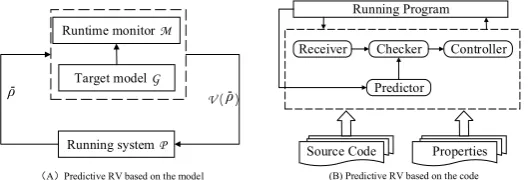
decision as early as possible. One of our previous work in predictive RV is based on system model, as 88

the framework shown in Figure1A.Gis the model of software to be monitored. During runtime, the 89

monitorMgenerated from LTL property will use the information of modelGto predict whether the 90

current system trace ¯ρwill violate the property in the future. When there exist violation paths from 91

current state, the active monitor will generate a corresponding intervention behaviorV(ρ¯)which can 92

guide the running to correct paths and feed it back to the running systemP. 93

（A）Predictive RV based on the model

V ( )

Running system P

Runtime monitor M

Target modelG

ρ- _ρ- Predictor

Receiver Checker Controller Running Program

Source Code Properties

(B) Predictive RV based on the code

Figure 1.Two types of existing predictive RV methods.

For software without models, we also proposed another predictive RV method which depends 94

on code static analysis [6], as shown in Figure1B. Control Flow Graph (CFG) of the code is extracted 95

before software is deployed. For each control node in CFG, the event sequences related to the property 96

in its scope are generated, and the variables whose values will be calculated at runtime and used 97

in branch decision expression are also recorded. At runtime, the monitor will predict the property 98

violation based on these event sequences and variable values at current state. Although the method 99

can predict the violation more accurately since branch decision is determined at runtime, the cost may 100

be huge for complex software. 101

One obvious shortcoming of above predictive RV methods is that they are not suitable for software 102

without models or codes, or systems running in uncertain environment. These problems will be focused 103

on in this paper. 104

2. Preliminaries 105

2.1. Linear-time Temporal Logic 106

Linear-time Temporal Logic (LTL) is usually used to specify the temporal behavior and properties of system. Assuming thatPis a set of atomic propositions, andΣ=2P denotes the finite alphabet, LTL formulae can be defined as

ϕ::= p| ¬ϕ|ϕ1∨ϕ2|Xϕ|ϕ1Uϕ2

wherep∈ P. There are some standard derived operators, such as: 107

> ≡ p∨ ¬p 108

ϕ1∧ϕ2 ≡ ¬(¬ϕ1∨ ¬ϕ2)

109

ϕ1→ϕ2 ≡ ¬ϕ1∨ϕ2

110

Fϕ ≡ >Uϕ 111

Gϕ ≡ ¬(F¬ϕ) 112

ϕ1Rϕ2 ≡ ¬(¬ϕ1U¬ϕ2)

Semantics of LTL formulae are defined with an infinite traceπ ∈Σωand a positioni. Thei-th 114

letterπ(i)of the traceπis a subset ofP, which can be viewed as an assignment toP. The standard 115

semantics of the LTL formulae are defined as follows [7]: 116

π,i |= p∈ P ⇔ p∈π(i)

π,i |= ¬ϕ ⇔ π,i6|= ϕ

π,i |= ϕ1∨ϕ2 ⇔ π,i|=ϕ1orπ,i|=ϕ2

π,i |= Xϕ ⇔ π,i+1|=ϕ

π,i |= ϕ1Uϕ2 ⇔ ∃j≥i:π,j|= ϕ2and ∀i6k<j:π,k|=ϕ1

2.2. RV and Monitoring Semantics 117

RV is a lightweight formal verification method that only focuses on whether the current execution 118

of system meets certain properties. At runtime, a system trace can be treat as a finite sequence 119

composed of system states, and different definitions of state should be given for different concerns. At 120

hardware level, the state of the system should be defined with the combination of values of registers, 121

memories and so on. At software level, the system state is usually defined by the locations of the 122

program, the values of variables, the events of function calling and so on. 123

The current system execution at runtime is a finite prefix of the infinite trajectory. The goal of RV 124

is to check whether this prefix satisfies the given property. Commonly a monitor will be generated 125

from the given property according to a specific method to do this checking. Thus, from perspective 126

of the formal language, RV solves the problem whether a given word is included in the language 127

corresponding to the given property. Therefore, the monitor is the device that reads a finite trace and 128

yields a certain verdict. 129

Monitoring semantics [15] is a set of advanced logical protocols that formally define what decision 130

the monitor makes in different situations. Different monitoring semantics may get different conclusions. 131

The standard semantics of LTL is defined on infinite traces, which can not be applied directly to finite 132

traces. For two-valued semantics of LTL, there are the following three methods to solve this problem 133

[16]. Given a finite traceµand a LTL formulaϕ, 134

(1) Weak semantics:ϕis violated iffµis a bad-prefix of it. Namely, for any infinite wordν, we 135

haveµν6|=ϕ. 136

(2) Strong semantics: In this case,ϕis satisfied iffµis a good-prefix of it. That is,µν|= ϕfor every 137

infinite wordν. 138

(3) Multi-value semantics: There exist consistency problems in two-valued semantics of LTL. Thus 139

multi-value semantics was proposed and defined on infinite trace, such asLTL3:

140

[µ|=ϕ]LTL3 =   

 

true, i f ∀σ∈Σω :µσ|=LTL ϕ; f alse, i f ∀σ∈Σω :µσ6|=LTL ϕ; ?, otherwise.

2.3. Discrete Time Markov Chain 141

Discrete Time Markov Chain is a stochastic process in mathematics for discrete events. In the 142

process, given the current state with knowledge or information, the historical state is not considered 143

when predict the future state. It is called markov-process. In addition, it is found that no matter what 144

state it is, the markov-process will gradually become stable after a period of time, and the state of 145

stability is not related to the initial state. 146

With a countable set P of propositions, a discrete time markov chain (DTMC) M is a tuple 147

• Sis a finite set of states; 149

• Iis an initial distribution overS, and

∑

• T:S×S→[0, 1]is the transition matrix fulfilling

∑

151

• L:S→2P is the labelling function. 152

3. Learning based Probabilistic Modelling 153

Event is usually used to encapsulate the behavior and interactions for many software systems, 154

and event-triggered RV is used to ensure the reliability of a system by observing the occurrence of 155

events. During the process of monitoring the target system running in specific environment, there is 156

a kind of events that seem to be independent of each other. However, there often exist some hidden 157

correlations among these events. 158

B A

C

r:100m

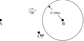
Figure 2.An example with uncertain environment in practice.

For example, as shown in the Figure2, a drone often flies from point Ato pointB, and there 159

is a control tower at pointCthat sends instruction to this drone. Event p is defined asthe drone 160

reaches the area within 100 meters around point B. The operator obtains the position information from the 161

drone and sends instructions through the control tower. In a real environment, the communication 162

between drone and control tower may be hindered by some obstacles, thereby leading to some flight 163

deviation. Another eventqis defined asthe drone sends the position information back to control tower C. 164

We have to monitor whether the mission can be completed successfully. On the surface,pandqare 165

independent events, but these events contain potential probabilistic relationships since the landform 166

such as mountains or interference sources nearby may affect the sending and receiving of information. 167

This case will also be used in the following when describing the proposed method. 168

Target system

Log Event Extraction

Path Join Processing Forward-Backward Algorithm

Log DataBase

HMM Log

Path Series path

Event name

Environment

Properties (LTL)

Translate HMM To DTMC

DTMC Log fragment

Figure 3.Framework of learning the model of target system and environment.

Figure3show the framework of learning the DTMC model of target system and environment. 169

First, event traces related to the monitoring property need to be extracted from the log history. Then 170

these paths are joint to form one trace from which the HMM will be learned according to the distribution 171

of their occurrence. Here the forward-backward algorithm in machine learning is adopted. Finally 172

HMM is transformed to DTMC, which will be used in monitor generation. 173

3.1. Problem Description 174

For the software without providing models and codes, running trajectory can be obtained from 175

trajectories from the log database to learn the model with the focus on eventspandq. The traces can 177

be expressed as the form such as: π =Sinit → p →p →q →p →∅ →∅→SEnd. The symbol∅

178

indicates that neitherpnorqoccur. porqseparately shows that corresponding event occur. Symbol 179

pqis used to represent the set{p,q}, which means the occurrence of both eventspandq. 180

Before formalizing the problem, some definitions need to be introduced. A finite traceπis a 181

string inΣ∗andlengthof the trace is denoted bylen(π). π(i)denote thei-thlocation ofπfor each 182

i<len(π); therefore,π(i)⊆ P. A DTMC is a stochastic process that satisfies the following provisos: 183

- Proviso_1: The probability distribution of the system state at timet+1 is only related to the state 184

at timetand is independent of the states beforet; 185

- Proviso_2: The state transition from timettot+1 is independent of the value oft. 186

Given a DTMCM= (S,I,T,L)and a traceπ, and[n]to denote the set{0, . . . ,n−1}forn∈N,

187

a mapping fromπtoMis defined as a functionδwith type[len(π)]→Ssuch thatL(δ(i)) =π(i). 188

Then, the probability ofπw.r.t.Munderδis defined as 189

probδ(M,π) =I(δ(0))·

∏

We denote by∆M,πthe set that comprises all mappings fromπtoM. We now calculate the value 191

sup_δ∈∆M,πprobδ(M,π)and the corresponding mapping. In other words, our goal is to find a mapping 192

δthat makesprob_δ(M,π)as large as possible. 193

We can canonically lift this problem when we are given a (finite) path setΠ. In this setting, our goal 194

is to determine a mappingδπ∈∆M,πfor eachπ∈Πand to maximize the value ofΣπ∈Πprobδπ(M,π). 195

There have been some methods can be used to solve this problem. In this paper, we propose a method 196

by learning a (HMM) model from traces to solve this problem. 197

3.2. Hidden Markov Model 198

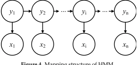
HMM is a directed dynamic Bayesian network diagram [17] with a simple structure that is mainly 199

used for timing data modeling, speech recognition, and natural language processing. As shown in 200

Figure4, HMM has two groups of variables. The first group is called the hidden or state variables 201

Y={y1, ...,yn}, whereyirepresents the hidden, unobservable state at time t= i. Assuming that the

202

number of all states in the model isN, that is, the state spaceY = {s1, ...,sN}, we haveyi ∈ Y. The

203

second group is called the observation variables or display statesX={x1, ...,xn}, wherexjrepresents the

204

state that can be observed directly att=j. The observed variables can either be continuous or discrete. 205

Here we only consider the discrete variables since the systems monitored in our work are supposed 206

discrete time systems. Assuming the number of observed variables ism, that is, the observation space 207

X = {o1, ...,om}, we havexj∈ X.

208

y

x

y

x

y

y

x

x

...

...

Figure 4.Mapping structure of HMM.

In Figure4, an arrow represents the dependency among variables. HMM has the following 209

properties: 210

- The change of hidden states is a DTMC, that is, process (y1→y2→...→yn) is consistent with

211

- The observed variablextis determined by the hidden variableytand is independent of other

213

observed or hidden variables. 214

Based on above independence relationship, the joint distribution ofXandYis 215

P(x1,y1, ...,xn,yn) =P(x1|y1)

n

∏

i=2

P(yi|yi−1)P(xi|yi)

216

217

If we want to determine a hidden Markov modelM, then the following parameters are required 218

in addition to the state spaceYand observation spaceX: 219

• Hidden state transition probability matrixA = [aij]N×N, whereaij = P(yt+1 = sj|yt = si),

220

1≤i,j≤N, which represents the probability of transitions between states in the model. 221

• Probability matrix of observationB= [bij]N×M, wherebij=P(xt=oj|yt=si), 1≤i≤ N, and

222

1≤j≤ M, which represents the observed probability from hidden to display states. In other 223

words,bijrepresents the probability that the observed valueojis observed at timet, if the hidden

224

state at this time issi.

225

• Initial distributionθ = (θ1, ...,θi, ...,θn), which is the probability of occurrence of each state at

226

timet=0, whereθi =P(y1=si)for 1≤i ≤ N. In other words,θiis the probability that the

227

initial state issi.

228

In practice, one of the basic problems that people often pay attention to HMM is how to learn 229

the optimal model parameters based on the sample set. It can be described as: given the observation 230

sequence x = {x1,x2, ...,xn}, how to learn the model parameter λ = [A,B,θ] to maximize the 231

probability of occurrence of sequenceP(x|λ)? Based on the traces we obtain from the log history, a 232

HMM need to be constructed that can best describe the observed data. 233

3.3. Learning Probabilistic Model 234

The most popular approach to constructing a HMM model is the forward-backward algorithm. 235

However, the forward-backward algorithm can only process one trajectory to construct HMM, so 236

multiple trajectories need to be combined for processing. First, we deal with all the traces obtained 237

from the log repository (the number of traces is assumed to beN). For example, if a traceπiappears a

238

total ofmitimes, we use pair(πi,mi)to represent them. The corresponding HMM synthesis algorithm

239

is presented in Algorithm 1. 240

Algorithm 1:HMM generation algorithm

Input:A finite settraces={(π1,m1),(π2,m2), . . . ,(πn,mn)}

Output:HMM modelHm

1 Π←ε; //Initialization ofΠas an empty string;

2 N=

n

∑

mi; //Nis the total number of traces

3 a←random(1,N); //ais a random value 4 forj←1toNdo

5 ifa∈[1+

k−1

∑

1

mk, k

∑

mk]then

6 Π←Π+πk; //πkis concatenated toΠ

7 a←random(1,N);

8 H_m=hmm(Π); // Call forward-backward algorithm; 9 returnH_m;

Merging all the traces directly will introduce errors into the final model and non-existent paths, 241

such as those transitions from the end states to the initial states. In this case, we add two states to all 242

resulting traces, namely,SinitandSend. The introduction of these two states will improve the accuracy

M = 6 N = 6

A:

0.001342 0.509898 0.487121 0.001781 0.001891 0.001989 0.001897 0.204231 0.275123 0.098343 0.423153 0.001176 0.001279 0.099123 0.281981 0.523891 0.095871 0.001891 0.001871 0.001898 0.001891 0.996891 0.001090 0.000123 0.000671 0.000211 0.001452 0.000983 0.998981 0.001981 0.001981 0.000781 0.000981 0.499901 0.499891 0.001771

B:

0.991842 0.001901 0.001981 0.001075 0.001981 0.001826 0.001781 0.991782 0.001092 0.001981 0.001887 0.001912 0.001089 0.001891 0.991091 0.001892 0.001891 0.001882 0.001901 0.001125 0.001091 0.989012 0.001192 0.001891 0.001193 0.001898 0.001098 0.008915 0.971881 0.001882 0.001183 0.001121 0.001781 0.009811 0.001982 0.991981

θ:

0.999986 0.001003 0.001003 0.001003 0.001003 0.001003

p q

Φ pq

0.20

0.28

0.10 0.42

0.28 0.10

0.52 0.10

1.00

0.51 0.49

1.00

Figure 5.The DTMC (Right) corresponding to the learned HMM (Left,Note that the matrixAcontains extra stateSinitandSend.), and the precision of data in DTMC is rounded to two decimals.

of the final model [18]. The classical forward-backward algorithm does not implement the incremental 244

process, fortunately, there is a lot of research to solve the problem, such as the work in [19]. 245

For example in Figure2, we simulate the process of generating DTMC in UAV platform Ardupilot 246

[20]. The data of all control commands and sensors are recorded into the log system of Ardupilot. We 247

implemented an event parser to obtain concerned events from logs. After simulating the flight for 248

10000 times, the corresponding traces are extracted and used to generate HMM with Algorithm 1. Left 249

part in Figure5depicts the HMM[A,B,θ]learned from 10000 traces, and the graphical representation 250

of its DTMC only containpandqis shown in the right part of Figure5. These logs are obtained by 251

monitoring the target drone and its environment. The DTMC model can be obtained from matrixAin 252

HMM directly. Through experiments, we find that the accuracy of the forward-backward algorithm is 253

closely related to two factors. First, a longer observation sequence corresponds to a higher accuracy. 254

Second, The similarity between the initial model and the target model will directly affect the efficiency 255

of the algorithm. 256

4. Probabilistic Monitor Generation 257

The generated DTMC is the model of system and environment learned, which should be used 258

together with the monitored property to determine and predict the satisfaction of property in specific 259

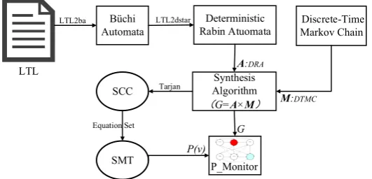
state. Thus, we will generate a probabilistic monitor from DTMC and the automaton corresponding to 260

the property. Figure6shows the framework of the procedures for generating probabilistic monitor. 261

Büchi Automata

Deterministic

Rabin Atuomata Discrete-TimeMarkov Chain

Synthesis Algorithm

（G=A×M）

SCC

SMT

LTL2ba LTL2dstar

Tarjan

Equation Set LTL

P_Monitor

A:DRA

M:DTMC

G

P(v)

Figure 6.The framework of probabilistic monitor generation.

ω-automata 262

Aω-automaton A= (Q,Σ,δ,Q0,Acc)includes the following elements:

263

• Qis a finite set of states; 264

• δ:Q×Σ→2Qis the transition function; 266

• Q0⊆Qis the initial state set;

267

• Accis the acceptance condition. 268

ω-automata can be classified into deterministic and non-deterministic ones, which mainly differ 269

in transition functions. An automaton is saiddeterministicif|Q0|=1 and|δ(q,a)|=1 for eachq∈Q 270

anda∈Σ. In this case, we consider the transition functionδto be of the typeQ×Σ→Q. 271

An input forAis an infinite string over the alphabetΣ, i.e. it is an infinite sequenceα=a0,a1,a2, ....

272

The run ofAon such input is an infinite sequenceρ=r0,r1,r2, ... of states, defined as follows:r0∈Q0

273

andri∈δ(ri−1,ai−1)wherei≥1. Letρdenote a run ofAover the infinite wordσ∈Σω, andIn f(ρ) 274

be the set of states occurring infinitely inρ. Given the different acceptance conditions,ω-automata can 275

be classified into different types such as: 276

• Büchi automata (BA): For accept state setF⊆Q,F∩In f(ρ)6=∅; 277

• Rabin automata (RA): For the set of pairs{(E1,F1),(E2,F2), ...,(Em,Fm)}, whereEi,Fi⊆Q, there

278

exists some 16i6mthatEi∩In f(ρ) =∅andFi∩In f(ρ)6=∅. 279

In this paper, we use NBA and DRA to designate nondeterministic Büchi automata and 280

deterministic Rabin automata, respectively. 281

Directed Graph and SCC 282

A directed graphGis a tuple(V,E), where: 283

• Vis a finite non-empty set of vertices; 284

• E⊆V×Vis a finite set of directed edges. 285

Give a directed graphG = (V,E), andV0 ⊆ V. If for each pair of verticesx,y ⊆ V0 there are 286

x→yandy→x, then we call the subgraph ofGcomposed by the node setV0as strongly connected 287

componentSCC V0. 288

Maximal SCC, BottomSCCsand IntermediateSCCs

289

IfSCC V0 ⊆ C⇒V0 = Cfor eachSCC CofG, then we considerSCC V0as maximal SCC and 290

denote it bySCCsV0.

291

If aSCCsV0exists inG= (V,E)andC=V\V0, for each vertexx ∈V0andy∈ C, there is no

292

x→yholds. We then call it BottomSCCs, denoted asBSCCsV0.

293

If node setV0 isSCCs, but it is notBSCCs, we say theV0 is an IntermediateSCCs, denoted as

294

MSCCs.

295

Then given the learned DTMC and the LTL property to be monitored, we will generate 296

probabilistic monitor according to the process shown in Figure6. 297

4.1. From LTL to DRA 298

Various methods of translating a LTL formula into an equivalent Büchi automaton have been 299

proposed in literatures. Unlike model checking, here we focus on the probability of property 300

satisfaction when a new event is observed, thus we hope the monitor should be deterministic. Since 301

deterministic Büchi automata are strictly less expressive than the non-deterministic ones, currently 302

there is no way for translating NBAs into DBAs. But, McNaughton’s Theorem and Safra’s construction 303

provide the algorithm that can translate a Büchi automaton into a deterministic Rabin automaton 304

[21]. Thus we will use DRA as the automaton formalism of LTL property, which still need BA as 305

intermediate representation. 306

The tool LTL2BA [22] can convert LTL formulas into Büchi automata. The conversion is 307

implemented in three steps. Firstly, the LTL formula is transformed into a very weak alternating 308

automaton (AWAA). This step mainly deals with the logical relations among the sub-formulas. 309

（B）The DTMC extracted from log library by machine learning method.

（C）Initial probability monitor M = DRA × DTMC （D）Optimized probability monitor obtained by merging 0 or 1 states （A）The DRA corresponding to the LTL formula FGp generated by LTL2dstar.

Figure 7.Generating probability monitor for propertyϕof UAS.

the problem of state combinations. Thirdly, GBA is converted into BA by using an easy-to-use and 311

well-known construction method. Finally, we use tool LTL2dstar [23] to convert BA into DRA with a 312

worst-case complexity of 2O(nlogn), wherendenotes the number of states in BA. 313

4.2. Generating Probabilistic Runtime Monitor 314

With the DTMC learned and the DRA constructed from property, we now can generate the 315

probabilistic monitor as follow. 316

Step1: Product of DRA and DTMC. Given a DRA A = (Q,Σ,δ,q0,ACC)and a DTMC M =

317

(S,I,T,L), where Σ = S, we firstly construct their production. Define the directed graph G = 318

A×M = (V,E), whereV = {(q,s)|q ∈ Q,s ∈ S}. An edgee∈ Ehas the forme = ((q,s),(q0,s0)), 319

which should satisfyT(s,s0)>0 andq0 =δ(q,s). Figure7presents an example of this construction 320

process, where the DRA is generated by the LTL formula ϕ = FGpwhich is a property should be 321

satisfied by the case in Figure2. 322

Step2: Probability Calculation. We useP(v)to denote the probability that nodev= (q,s)∈V 323

will satisfy the LTL property in finite graphG. In order to calculate the probability of each node in 324

G, the concept ofAccepted_SCCsis introduced. The acceptance condition of the DRA generated by

325

LTL isACC={(E1,F1), ...,(Ek,Fk)}. ABSCCsCisacceptedif there is someisuch thatC∩Ei =∅and

326

C∩Fi6=∅. Otherwise theBSCCsCisrejected. For nodev= (q,s)inSCCsC, its probability will be

327

(1) IfCis anAccepted_SCCsthenP(v) =1;

329

(2) IfCis anRejected_SCCsthenP(v) =0;

330

(3) IfCis anIntermediate_SCCsthenP(v) =∑u∈W(T(s,s0)×P(u)),Wis set of all successors ofv,

331

anduis denoted as(q0,s0)whereq0=δ(q,s). 332

We use the case in Figure 7 to describe the procedures. Figure 7A and 7B present the DRA and 333

DTMC which are input of algorithm 1. Figure 7C gives the product of them. The initial states are 334

nodes(S2,p)and(S2,q), then we can obtain allSCCsusing the classic Tarjan algorithm and we name

335

itFindSCCs. As shown in Figure7C, except for nodes(S2,p),(S2,q),(S1,q),(S1,p),(S0,p),(S0,q)

336

that make up oneSCCs, every other node is aSCCs.

337

According to the previous definition, we can easily know that node(S0,pq)and node(S2,∅)

338

areBSCCs. Based on the definition of Accepted_BSCCs and the DRA structure, we can work out

339

the probability ofAccepted_BSCCs(S0,pq)with above (1) andRejected_BSCCs(S2,∅)with (2). For

340

all MSCCs, we obtainPby solving the equations based on (3). For instance, we can calculate the

341

probability of nodes in oneMSCCswith following equations:

342

P(S0, p) = P(S0,p)∗T(p,p) +P(S0,pq)∗T(p,pq) +P(S2,q)∗T(p,q) +P(S2,∅)∗T(p,∅)

P(S0, q) = P(S2,p)∗T(q,p) +P(S2,∅)∗T(q,∅)

+P(S2,pq)∗T(q,pq) +P(S2,q)∗T(q,q)

P(S1, p) = P(S0,p)∗T(p,p) +P(S0,pq)∗T(p,pq)

+P(S0,∅)∗T(p,∅) +P(S0,q)

P(S1, q) = P(S2,p)∗T(q,p) +P(S2,q)∗T(q,q)

+P(S2,∅)∗T(q,∅) +P(S2,pq)∗T(q,pq)

P(S2, p) = P(S1,p)∗T(p,p) +P(S1,pq)∗T(p,pq)

+P(S2,q)∗T(p,q) +P(S2,∅)∗T(p,∅)

P(S2, q) = P(S1,pq)∗T(q,pq) +P(S1,p)∗T(q,p)

+P(S2,q)∗T(q,q) +P(S2,∅)∗T(q,∅)

The above equations are solved usingGaussian− Eliminationmethod and the probability of each 343

node can be obtained then. As show in these equations, to calculate the probability of node(S2,q), we

344

should know the probability of node(S2,∅)which we have worked out before. So in fact the process

345

of the calculation is Depth-First-Search (DFS) which consists with the process of Tarjan algorithm. 346

Because of this fact, once we find aSCCsthrough the Tarjan algorithm, we can calculate the probability

347

of each node in thisSCCswhich meet formulaϕ=FGp, as shown in Figure7C. 348

Step3: Optimization. After calculating the probability of each state based onG= A×M,Gand 349

the labelled probability make up the runtime monitor. For some states in the monitor, the probability 350

labels are 0 or 1. These states can be merged to optimize the structure of the monitor. In this example, 351

given that the probability labels for states(S0,pq) and(S1,pq)are both 1, they can be merged to

352

optimize the monitor as shown in Figure7D. 353

5. Implementation and Evaluation 354

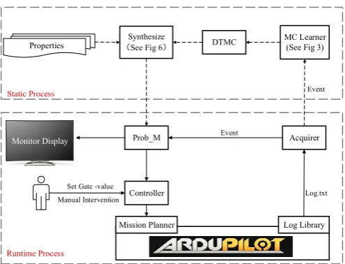
The tool framework and running process of the probabilistic runtime monitor is briefly described 355

in Figure8. It extracts the events of interest from event acquirer module. When an event occurs, 356

the probabilistic monitor will perform a transition based on its current state and the recieved event. 357

Based on the system requirements, if the probability value exceeds our specified gate value, then some 358

events labelled on the transitions in the monitor following current state can help controller to change 360

the direction of the system running by trigger a specific event. 361

Properties DTMC MC Learner(See Fig 3)

Synthesize （See Fig 6）

Prob_M Acquirer

Controller Static Process

Runtime Process

Event

Event

Log.txt

Mission Planner Log Library

Monitor Display

Set Gate -value Manual Intervention

Figure 8.The framework of tool implementation in the UAS simulation platform Ardupilot.

In the process of running the system, theAcquirerobtains the events from the target system and 362

environment, andProb_Mis the main part of the monitor platform which stores the structure of the 363

monitor and changes its state based on the event obtained by Acquirer. TheControllerdecides which 364

control event should be issued in next step when the system encounters a problem, or prompts what 365

external command intervention are needed to maintain the system in safe state. In the static phase, we 366

can use the traces newly added to the log library to update the learned model, which can continuously 367

improve the accuracy of the probabilistic monitor. 368

Compared with our work, traditional RV monitor under binary semantics of LTL faces the 369

semantic problem of consistency, since they should give a new semantics of LTL on finite traces. 370

Although the monitoring method under three-valued semantics of LTL can satisfy impartial and 371

anticipatory requirements [7], the monitor does not produce more quantitative results when the 372

satisfaction of property in many states are output as "?" (inconclusive). Meanwhile, the probabilistic 373

monitor can exactly determine the quantitative evaluation of satisfying the LTL property in current 374

state, thereby greatly expanding its application scenarios and making up the insufficiency of other RV 375

methods. 376

Furthermore, our probabilistic monitors can adjust the subsequent execution of the target system. 377

Specifically, when the system is running, people know which “event" can increase or decrease the 378

future probability for the system to meet the property. The existing runtime monitors are unable to 379

achieve this purpose. 380

To show the effectiveness of the method proposed above, we applied the probabilistic RV and its 381

tool to actual UAS platform Ardupilot. It is generally known that the hardware or software defects 382

and the presence of external malicious attacks pose a great threat to the security of UAS. Let’s consider 383

the following situation. 384

When UAS reconnaissances a hostile force area, if it encounters dangerous conditions (such as abnormal 385

signal interference), in order to balance the task completion and UAS safety, we set the following rules: Firstly, 386

if detection task has been initialized, the drone will not accept abnormal signal (both from the region and the 387

console), until the task has finished or the task is interrupted (such as receiving a normal command of stopping 388

detection); Secondly, if the task has not been initialized after enter this hostile area, the task will not be started to 389

Therefore, we define the following events: (1)p: the UAS is in the state of executing critical task, and (2)q: the UAS has received abnormal instruction. Then the property can be expressed by LTL formula:

ϕ=G((p→(¬qU¬p))∧(¬p→G¬p))

（A）The DRA corresponding to the LTL formula：φ = G((p → (!qU!p)) ∧ (!p → G!p)) . （B）The DTMC model extracted from UAV log Library.

（C）Probability monitor generated by the algorithm in this paper. （D）The monitor generated by tool LTL3tools is based on _{three-value semantics of LTL.}

Figure 9. The experiments of probability monitor compared with monitor based on three-value semantics.

The corresponding DRA of propertyϕis generated and shown in figure9A, and the DTMC model 391

(based on propositionspandq) of this UAS is obtained by learning the log history of multiple flight 392

simulations, which is shown in figure9B. The probabilistic monitor is generated from above DRA and 393

DTMC as shown in figure9C. Depend on this monitor, 200 system running traces with length 1000 394

(in fact the trace should be infinite, here length 1000 can embody the effectiveness of the method) are 395

checked whether they satisfied this safety property. As the result, there are 140 traces finally arrive the 396

state with probability 1.000 that satisfies the property, and for the left 60 traces the probability is 0.000. 397

The ratio of the traces satisfying the property in all traces is 70%, which is close to the probability on 398

the initial node with the probability 72.59%. 399

To compare with our method, similar experiments with same data is conducted under the 400

semantics ofLTL3. Firstly, the same LTL formula is transformed into the monitor shown in figure??

401

D by applyingLTL3tool. Obviously, there is no state oftruein this monitor because the formula is

402

begin with operatorG, andtruecannot be obtained in infinite word under the semantics ofLTL3. It is

403

becauseLTL3method does not consider the environment that system runs in. But our probabilistic

404

monitor learned the model from history of both system and environment, and use these information in 405

the monitor. By repeating the same 200 traces, theLTL3monitor get the results with 140 uncertain and

406

current safety status, but also the probability when it is running in uncertain environment, which takes 408

the advantage of Markov chain. 409

6. Conclusion 410

For the system without accurate model and program code, or running in the uncertain 411

environment that threaten cannot be predicted before deployment, we propose an approach to 412

constructing probabilistic monitor to detect property violation at runtime. The method utilizes the 413

history traces from the log repository of target system to learn the HMM model which represents the 414

behavior of both system and environment. Then the DTMC model is obtained from HMM. Together 415

with the DRA generated from LTL formula, the probabilistic runtime monitor can be generated after 416

calculating the probability of state in the product of DTMC and DRA. Probabilistic monitor has a good 417

application scenario in which the LTL property originally cannot be quantitatively judged with existing 418

RV methods, and it also can provide directional guidance for system intervention. We implemented 419

the corresponding tool on the UAS platform Ardupilot, and the experiments show the effectiveness 420

comparing with other methods such asLTL3.

421

In the future work, we plan to study the method of building probabilistic monitor with online 422

incrementally learning, so that when the target system’s log library grows, the model learned can 423

become more accurate in time. Furthermore, for the probabilistic monitor containing guidance 424

information, we will study an effective intervention mechanism. 425

References 426

1. Zhang, P.; Su, Z.; Zhu, Y.; Li, W.; Li, B. WS-PSC Monitor: A Tool Chain for Monitoring Temporal and

427

Timing Properties in Composite Service Based on Property Sequence Chart. International Conference,

428

2010, pp. 485–489.

429

2. Electrical, I.O.; Board, I.S. IEEE Standard for Software Verification and Validation. Software Quality 430

Professional2005, pp. 1–217.

431

3. Clarke, E.M. Model Checking-My 27-Year Quest to Overcome the State Explosion Problem. Logic in

432

Computer Science, 2009. LICS ’09. IEEE Symposium on, 2008, pp. 3–3.

433

4. Dahl, O.J.; Dijkstra, E.W.; Hoare, C.A.R.Structured programming; Academic Press, 1972; pp. 179–185.

434

5. Zhao, C.; Dong, W.; Wang, J.; Sui, P.; Qi, Z. Software active online Monitoring under anticipatory Semantics.

435

Shm2009.

436

6. Yu, K.; Chen, Z.; Dong, W. A Predictive Runtime Verification Framework for Cyber-Physical Systems.

437

IEEE Eighth International Conference on Software Security and Reliability-Companion, 2014, pp. 247–250.

438

7. Bauer, A.; Leucker, M.; Schallhart, C. Comparing LTL Semantics for Runtime Verification. Journal of Logic 439

& Computation2010,20, 651–674.

440

8. Naskos, A.; Stachtiari, E.; Katsaros, P.; Gounaris, A.Probabilistic Model Checking at Runtime for the Provisioning 441

of Cloud Resources; Springer International Publishing, 2015; pp. 275–280.

442

9. Filieri, A.; Tamburrelli, G.Probabilistic Verification at Runtime for Self-Adaptive Systems; 2013; pp. 30–59.

443

10. Nouri, A.; Raman, B.; Bozga, M.; Legay, A.; Bensalem, S. Faster Statistical Model Checking by Means of

444

Abstraction and Learning. Runtime Verification, 2014, pp. 340–355.

445

11. Sammapun, U.; Lee, I.; Sokolsky, O.; Regehr, J.Statistical Runtime Checking of Probabilistic Properties; Springer

446

Berlin Heidelberg, 2007; pp. 164–175.

447

12. Ngo, V.C.; Legay, A.; Joloboff, V. PSCV: A Runtime Verification Tool for Probabilistic SystemC Models2016.

448

13. Jayaputera, J.; Poernomo, I.; Schmidt, H. Runtime Verification of Timing and Probabilistic Properties using

449

WMI and .NET. Euromicro Conference, 2004. Proceedings., 2004, pp. 100–106.

450

14. Zhao, C.; Dong, W.; Qi, Z. Active Monitoring for Control Systems under Anticipatory Semantics.

451

International Conference on Quality Software, 2010, pp. 318–325.

452

15. Chen, Z.; Wei, O.; Huang, Z.; Xi, H. Formal Semantics of Runtime Monitoring, Verification, Enforcement

453

and Control. International Symposium on Theoretical Aspects of Software Engineering, 2015, pp. 63–70.

454

16. Giannakopoulou, D.; Havelund, K. Runtime Analysis of Linear Temporal Logic Specifications. 2001.

17. Chu, S.M.; Huang, T.S. An experimental study of coupled hidden Markov models. IEEE International

456

Conference on Acoustics, Speech, and Signal Processing, 2002, pp. IV–4100–IV–4103.

457

18. Abbasi, N.M. Hidden Markov Methods. Algorithms and Implementation2015.

458

19. Motik, B.; Nenov, Y.; Piro, R.; Horrocks, I. Incremental update of datalog materialisation: the

459

backward/forward algorithm. Twenty-Ninth AAAI Conference on Artificial Intelligence, 2015, pp.

460

1560–1568.

461

20. An simulation platform of unmanned aerial vehicle. http://www.ardupilot.org/.

462

21. Safra, S. On the complexity ofω-automata. Foundations of Computer Science, 1988., Symposium on, 1988,

463

pp. 319–327.

464

22. Gastin, P.; Oddoux, D. Fast LTL to Büchi Automata Translation. International Conference on Computer

465

Aided Verification, 2001, pp. 53–65.

466

23. LTL to deterministic Streett and Rabin automata. http://www.ltl2dstar.de/.