Article
An
A
lgorithm
for
N
onparametric
E
stimation
of
A
M
ultivariate
M
ixing
D
istribution
with
A
pplications
to
P
opulation
P
harmacokinetics
WalterM.Yamada1,‡ ,MichaelN.Neely1,2,‡,JayBartroff8,‡,DavidS.Bayard1,3,‡,JamesV.
Burke4,‡,MikevanGuilder1,‡,RogerW.Jelliffe1,‡,AlonaKryshchenko1,5,‡,RobertLeary6,‡,
TatianaTatarinova7,‡,andAlanSchumitzky1,8,*
1 Laboratory of Applied Pharmacokinetics and Bioinformatics, Children’s Hospital of Los Angeles, Los Angeles, CA 90027, USA;
2 Pediatric Infectious Diseases, Children’s Hospital of Los Angeles, Keck School of Medicine, University of Southern California, Los Angeles, CA 90027, USA;
3 Jet Propulsion Laboratory, California Institute of Technology, Pasadena CA, 91109, USA; 4 Department of Mathematics, University of Washington, Seattle, WA 98195, USA;
5 Department of Mathematics, California State University Channel Islands, University Dr, Camarillo, CA 93012, USA;
6 Certara, Raleigh, NC 27606, USA;
7 Department of Biology, University of La Verne, La Verne, CA 91750, USA;
8 Department of Mathematics, University of Southern California, Los Angeles, CA 90089, USA; * Correspondence: [email protected]; Tel.: +1 818-249-9444
‡ These authors contributed equally to this work.
1
2
3
4
5
6
7
8
9
10
11
12
13
Abstract:
Inthispaperwedescribeanonparametricmaximumlikelihood(NPML)methodforestimating multivariatemixingdistributions.GivenNindependentobservations,convexitytheoryshowsthat theNPMLestimatorisdiscretewithatmostNsupportpoints.TheoriginalinfiniteNPMLproblem thenbecomesthefinitedimensionalproblemoffindingthelocationandprobabilityofthesupport points.TheprobabilityofthesupportpointsisfoundbyaPrimal-DualInterior-Pointmethod;the locationofthesupportpointsisfoundbyanAdaptiveGridmethod.Ourmethodisabletohandle high-dimensionalandcomplexmultivariatemixturemodels.Animportantapplicationisdiscussed fortheproblemofpopulationpharmacokineticsandanon-trivialexampleistreated.Ouralgorithm hasbeensuccessfullyappliedinhundredsofpublishedpharmacometricstudies. Inadditionto populationpharmacokinetics,thisresearchalsoappliestoempiricalBayesestimationandmany otherareasofappliedmathematics.
Keywords: mixture distribution; mixture model; high dimensional statistics; nonparametric
maximum likelihood; primal-dual interior-point method; adaptive grid 14
1. Introduction
15
Pharmacometric observations can be described statistically by a mixture model. In this case, the probability of random variable arguments (the PK population model) of the pharmacokinetic compartmental model are described by a mixing distribution. The problem of estimating the mixing distribution from a set of pharmacometric observations can be stated as follows. LetY1, ...,YN be a sequence of independent but not necessarily identically distributed random vectors constructed from one or more observations from each ofNsubjects in the population. Letθ1, ...,θNbe a sequence of
independent and identically distributed random vectors belonging to a compact subsetΘof Euclidean space with common butunknowndistributionF. The{θi}are not observed. It is assumed that the conditional densitiesp(Yi|θi)are known, fori=1, ...,N. The mixing distribution ofYiwith respect to Fis given byp(Yi|F) =R p(Yi|θi)dF(θi). Because of independence of the{Yi}, the mixing distribution of the{Yi}with respect toFis given by
L(F) =p(Y1, ...,YN|F) = N
∏
i=1 Zp(Yi|θi)dF(θi) (1)
The mixing distribution problem is to maximize the likelihood function L(F)with respect to all probability 16
distributions F onΘ. 17
Remark. The distributionFMLthat maximizesL(F)is aconsistentestimator of the true mixing 18
distribution. This was proved originally by Kiefer and Wolfowitz in 1956 [1] . The consistency ofFML 19
is especially important for our application to population pharmacokinetics whereFMLis used as a 20
prior distribution for Bayesian dosage regimen design. 21
The algorithm described in this paper differs from most other published methods in a number of 22
ways. Our algorithm allows for high dimensionalΘ. Most published methods require the dimension of 23
Θto be small and many require the dimension ofΘto be 1, see Section1.1. We have treated examples 24
where the dimension ofΘis as high as 29, see Section3. 25
Also most published algorithms require the{Yi}to be identically distributed and assume that the 26
conditional densities{p(Yi|θi)}are rather simple, such asp(Yi|θi)is a multivariate normal density 27
with mean vectorθiand covariance matrixΣ. Even ifΣis unknown and has to be estimated, the 28
structure of this model is straightforward. However, the estimation ofΣhas to be done carefully to 29
avoid singularities, see Wang and Wang [2]. As will be described in Section3, we allowp(Yi|θi)to be 30
calculated from a system of nonlinear ordinary differential-algebraic equations. 31
We now describe the details of our algorithm. It was proved by Lindsay [3] and Mallet [4] , under simple hypotheses on the conditional densities{p(Yi|θi)}, that the global maximizerFMLof L(F)could be represented by a discrete distribution with at mostNsupport points. This result leads immediately to a finite dimensional optimization problem forFML, namely to maximize the likelihood function
L(λ,φ) = N
∏
i=1K
∑
k=1λkp(Yi|φk) (2)
with respect to the support pointsφ= (φ1, ...,φK)and weightsλ= (λ1, ...,λK)such thatφk∈Θ,λk ≥ 32
0 fork=1, ...,K,K≤Nand ∑K
k=1λk=1. 33
In our algorithml(λ,φ) =logL(λ,φ)is maximized, so that
l(λ,φ) = N
∑
i=1log K
∑
k=1λkp(Yi|φk) (3)
and the maximization problem becomes
maximizel(λ,φ) (4)
such thatφ∈ΘK,λ= (λ1, ...,λK)∈RK+,K≤Nand ∑Kk=1λk=1. 34
Although the maximization problem in Eq. (4) is finite dimensional, it is still high dimensional. 35
The dimension of the maximization problem in Eq. (4) isN(dimΘ) + (N−1). 36
The optimization problem in Eq. (4) is naturally divided into two problems: 37
Problem 1. Given a set of support points{φk}, find the optimal weights{λk}. 38
Problem 2. Given the solution to Problem 1, find a better set of support points. 39
Problems 1 and 2 are solved cyclically until convergence, i.e. no significant improvement in 40
Problem 1 is a convex programming problem. In our algorithm, we solve this problem by the 42
Primal-Dual Interior-Point (PDIP) method. This type of method is standard in convex optimization 43
theory, see Boyd and Vandenberghe [5]. However, the exact implementation for a specific problem 44
varies from problem to problem. The exact details of our implementation is described in the Appendix. 45
See also Bell [6], Baek [7] and Yamadaet al.[8]. Our PDIP implementation is very fast and can easily 46
handle thousands of variables. 47
Finding a better set of support points in Problem 2 is a more difficult problem. This location 48
problem is a non-convex global optimization problem with many local extrema and whose dimension 49
is potentialyN×dimΘ. The details of our algorithm, called the Adaptive Grid (AG) method, will be 50
described in Section2.3and in Algorithm 1. 51
Roughly speaking, Problems 1 and 2 are solved as follows. An initial large grid of possible 52
support points is defined inΘ. Problem 1 is solved on this large grid. After PDIP, most of the original 53
grid points are removed due to near-zero weights leaving a smaller high-probability grid. Problem 1 54
is then solved on this smaller grid. Then the Adaptive Grid method for Problem 2 takes place. For 55
each remaining grid point, up to 2×dimΘnew (daughter) support points are added. A daughter 56
point outside the search spaceΘor too close to a parent point is discarded. The new grid contains 57
the current high-probability points plus the added daughter points. The algorithm is then ready for 58
Problem 1, again. By construction, each iteration increases the value ofl(λ,φ). This process continues 59
until the functionl(λ,φ)does not significantly change. 60
1.1. Other algorithms 61
Because of space limitations, in this section we only discuss NPML methods that optimize 62
Eq.4; methods that treat multivariate distributions; and methods which allow general conditional 63
probabilities{P(Yi,θi)}. As explained in this paper, any such NPML algorithm has to address two 64
problems: locations of support points andweights of support points. NPAG doeslocations by an 65
Adaptive Grid method andweightsby the Primal-Dual Interior-Point (PDIP) method. 66
The original methods of Lindsay [3] and Mallett [4] were based on algorithms of optimal design 67
in the style of Fedorov [9]. In Schumitzky [10], an algorithm was proposed which did bothlocations 68
andweightsby the EM algorithm. It was very stable but also very slow. 69
In Lesperance and Kalbfleisch [11], a new method was introduced which didweightsby the dual 70
method described in Section 5 of Lindsay [3] andlocations by what they called the Intra-Simplex 71
Direction Method (ISDM). Even though, the Lesperance and Kalbfleisch paper was restricted to 72
univariate distributions, the ISDM method has been generalized to the multivariate case. To briefly 73
describe ISDM, let D(θ,F) be the directional derivative of logL(F) in the direction of the Dirac 74
distributionδθsupported atθ∈Θ. (This function is defined in Section 4 below.) ISDM is an iterative
75
algorithm. At stagek, letFkbe the current estimateFML. Then find all the local maxima ofD(θ,Fk). 76
These local maxima are added to the current set of support points and a newFk+1is calculated. If 77
there are no new local maxima, then the algorithm is done. 78
In Pilla, Bartolucci, and Lindsay [12], another new method was developed where thelocations 79
were found by an initial fine grid. But theweightswere found by a dual version of the PDIP method. 80
In Savic, Kjellsson, and Karlsson [13], a nonparametric method was added to the popular 81
NONMEM program. NONMEM-NP is a hybrid parametric-nonparametric approach Thelocations 82
of support points were found by a parametric maximum likelihood algorithm. Then theweights 83
were found by maximizing Eq. (4) relative to the newly found support points. NONMEM-NP can 84
handle high dimensional and complex multivariate distributions. An extension to NONMEM-NP was 85
developed in Savic and Karlsson [14] where additional support points are added to the original set. A 86
comparison between NONMEM-NP and NPAG is discussed in Leary [15]. 87
In Wang and Wang [2] , a new algorithm was developed for multivariate distributions. The 88
family of Quadratic Programs. In [2], examples are done for 8 and 13 dimensional mutivariate mixing 90
distributions. 91
Note: The Quadratic Programming algorithm (QP) of Wang and Wang [2] has a very attractive 92
feature. For a prescribed set of support points, QP finds the zero probabilities exactly. Thus QP avoids 93
the Grid Condensation step where support points from PDIP with sufficiently low probabilities are 94
deleted. However, QP and PDIP are based on different numerical methods and a comparison of the 95
efficiency of both algorithms has not been determined. 96
We finally mention that the NPML problem is a special case of a finite mixture model problem 97
with unknown supports and weights. For a discussion of this approach see Tatarinova and Schumitzky 98
[16]. 99
The algorithms which have shown by published examples to handle the highest dimensional 100
multivariate problems are NONMEM NP, Wang and Wang [2], and NPAG. 101
1.2. Benders Decomposition 102
For any set of grid pointsφ = (φ1, ...,φm)inΘm, letλ = λˆ(φ)be the corresponding set of 103
optimal weights given by the PDIP method. Then the functionF(φ) = l(λˆ(φ),φ)depends only 104
onφand can be maximized directly. For optimization methods, this technique is called Benders 105
Decomposition. The NPAG algorithm maximizesF(φ)by an adaptive search method. In a method 106
proposed by James Burke,F(φ)is maximized by a Newton type method. Since the functionF(φ) is 107
not necessarily differentiable, a relaxed Newton method must be used similar to what is described in 108
the Appendix for the Primal-Dual Algorithm. For details of Benders Decomposition as applied to our 109
problem, see Bell [6], Baek [7] and Jordan-Squire [17]. 110
2. Materials and Methods
111
2.1. Pmetrics 112
The simulations and NPAG optimizations in this paper can be duplicated in R, using programs in 113
the Pmetrics package [18]. R and Pmetrics are free software. R is available from many download sites. 114
Pmetrics is available from lapk.org. NPAG is run using the NPrun() command in Pmetrics. Sample 115
datasets and compartmental models are also available at lapk.org. 116
2.2. NPAG Subprograms 117
NPAG is a Fortran program consisting of a number of subroutines as described below. The 118
main program performs the Adaptive Grid (AG) method (consisting of expansion and compression 119
algorithms) and calls the Primal-Dual Interior-Point (PDIP) subprogram. The PDIP algorithm solves 120
the maximization problem of Eq. (4) for a fixed grid and is described precisely in the Appendix. 121
2.3. NPAG Implementation (NPAG - Algorithm 1) 122
For the purpose of this discussion, we can think of PDIP as a functionλˆ fromΘminto the setSm= 123
{λ ∈Rm+ :∑mk=1λk =1}defined as follows: Ifφ= (φ1, ...,φm)thenλˆ(φ) = (λˆ1, ..., ˆλm)maximizes 124
Eq. (4) relative to the fixed set of grid points(φ1, ...,φm). In this case we writeG=(φ,λˆ(φ))andl(G) 125
=l(φ,λˆ(φ)). 126
In NPAG there are two types of grids: expanded and condensed. The expanded grids are the 127
initial grid and the grids after Grid Expansion (Algorithm 2). The condensed grids are generated by 128
Grid Condensation (Algorithm 3). Each cycle of NPAG begins with an expanded grid. The likelihood 129
calculation is done on the condensed grids. 130
Now for the Adaptive Grid method. Assume thatΘis a boundedQ-dimensional hyper-rectangle. 131
we could initially letφ0expandedbe generated by a uniform distribution onΘor by a prior run of the 133
program. 134
Remark. The Faure grid points for a hyper-rectangleΘare a low-discrepancy set which in some 135
sense optimally and uniformly coversΘ. In our implementation of NPAG, the Faure point sets come in 136
discrete sizes which nest with each other. (Allowable number of points equals 2129, 5003, 10007, 20011, 137
40009, 80021, and multiples of 80021.) This nesting property is useful for checking the optimality of 138
FML, see Section 4. We have found that replacing the initial Faure set by a set generated by a uniform 139
distribution onΘincreases the time to convergence but results in the same optimal distribution. 140
Now setG0expanded=(φ0,λˆ(φ0)). Our approach is to generate a sequence of solutionsGnto Eq. 141
(4) of increasingly greater likelihood, where unless otherwise specified,Gnrefers to the condensed 142
grid at thenthcycle of the algorithm. IfGnhas log likelihood negligibly different thanGn−1, thenGn 143
is considered the optimal solution to Eq. (4) and is relabeledFML. If not, then the process continues 144
using theφnas the new seed. This loop is repeated untilFMLis found. 145
The stopping conditions for NPAG are defined precisely in Algorithm 1. If the stopping conditions 146
are not met prior to a set maximum number of iterations, the program will exit after writing the last 147
calculatedGninto a file. 148
2.4. Grid Expansion (EXPAND - Algorithm 2) 149
The crux of the Adaptive Grid method is how to go fromG0toG1or more generally, fromGnto 150
Gn+1. The details of doing this are now explained roughly below and precisely in Algorithm1. 151
LetQbe the dimension ofΘ. Suppose at stagenwe have a grid of high-probability support 152
pointsφn. We then add 2Qdaughter points for each support pointφk∈φn. The daughter points are 153
the vertices of a small hyper-rectangle centered at eachφkwith size proportional to the original size of 154
the hyper-rectangle definingΘ. The size of this small hyper rectangle decreases as the accuracy of the 155
estimates increases. (See Algorithm 2.) 156
Letφnexpanded+1 =φn∪Daughter-Points. Then the PDIP subprogram is applied toφexpandedn+1 resulting 157
in the new solution setGexpandedn+1 =(φnexpanded+1 ,λˆ(φexpandedn+1 )); see Algorithm1. The solution setGexpandedn+1 158
is now ready for grid condensation. 159
2.5. Grid Condensation (CONDENSE - Algorithm 3) 160
The above solution setGexpandedn+1 may have many support points with very low probability. We 161
remove all support points which have corresponding probability less than(maxλ)∆λ, whereλis the
162
vector of current probabilities and the default for∆λis 10
−3. (Note that at this point the remaining 163
probabilities are not normalized.) The probabilities of the remaining support points are normalized 164
by a second call to the PDIP subprogram. This second call to PDIP is very fast. The likelihood 165
associated with these remaining support points and normalized probabilities is then used to update the 166
program control parameters and check for convergence (Algorithm1and Section2.7). If convergence 167
is attained, then the output of this second call to PDIP provides the support points and probabilities 168
of the final solution. If convergence is not attained, then the remaining support points are sent to the 169
Grid Expansion subprogram (Algorithm 2), initializing the next cycle. 170
At the end of the program, the output of this second call to PDIP provides the location and 171
weights of the final solution. 172
2.6. PDIP Subprogram - See Appendix A 173
The PDIP subprogram finds the optimal solution to Eq. 4with respect toλfor fixedφ. PDIP 174
employs a primal-dual interior-point method that uses a relaxed Newton method to solve the 175
corresponding Karush-Kuhn-Tucker equations. (See Eqs. 14 -17 of Appendix A.) 176
For anyY=(Y1, ...,YN) and anyφ=(φ1, ...,φK) ∈ ΘK, the input to the PDIP subprogram is the 177
log-likelihoodl(λˆ(φ),φ). An in-depth description of the PDIP algorithm and its implementation is 179
presented in Appendix A. See also [6–8]. 180
2.7. NPAG Stopping Conditions 181
As explained above, apotentialsolution toFMLis not accepted as a global optimum until successive 182
sequences ofGnproduce final distributions evaluating to sufficiently close log likelihood. The various 183
upper and lower bounds∆for NPAG control and stopping conditions are defined below and are used 184
in Algorithms 1, 2, and 3. 185
∆L Primary upper bound on the allowable difference between two successive estimated 186
Log-Likelihoods; the default initialization is 10−4. 187
∆F Secondary upper bound on the allowable difference between two successive estimated 188
Log-Likelihoods ofpotential FML; the default initialization is 10−2. 189
∆e Sets an upper bound on the accuracy variableepsof Algorithm 1. The default initialization for 190
∆eis 10−4. The default initialization forepsis 0.2 and is stepped down untileps≤∆e 191
∆Fand∆edefine the two stopping conditions for Algorithm 1. 192
∆D Sets a lower bound on how close two support points can get; the default initialization is 10−4. 193
∆λ Sets a lower bound factor on the probabilities of the weightsλ; the default initialization is 10 −3. 194
2.8. Calculation of p(Yi|φk) 195
Given observationsYi,i = 1, ...,Nand grid pointsφk,k =1, ...,K, the PDIP subprogram only 196
depends on theN×Kmatrix{p(Yi|φk)}. NPAG can be used for any problem once this matrix is 197
defined. However, the default setting of NPAG is for the problem of population pharmacokinetics. For 198
a good background of population pharmacokinetics see Davidian and Giltinan [22,23]. 199
In population pharmacokinetics, generallyYi = (yi,1, ...,yi,M)is a matrix of vector observations for the i-th subject. Since NPAG allows multiple outputs, eachyi,mis itself aq-dimensional vectoryi,m =(yi,m,1,· · ·,yi,m,q). The observationsyi,m,j, are then typically given by a regression equation of the form:
yi,m,j= fi,m,j(θi) +νi,m,j, j=1,· · ·,q (5)
νi,m,j∼N(0,(σi,m,j(θi))2)
θiare unobserved parameters specific forYi
In the above Eq. 5, fi,m,jis a known nonlinear function depending on the model structure, the dosage 200
regimen, the sampling schedule, all covariates and of course the subject-specific parameter vector 201
θi. Except for simple models, fi,m,jrequires the solution of (possibly nonlinear) ordinary differential 202
equations. 203
In the current implementation of NPAG, it is assumed that the(yi,1, ...,yi,M)are independent. Then
p(Yi|φk) =
exp −1
2 M
∑
m=1(yi,m− fi,m(φk))Σ−i,m1(φk)(yi,m−fi,m(φk))T
!
∏M m=1
p
(2π)qdetΣi,m(φk)
(6)
where fi,m= (fi,m,1, ...,fi,m,q)andΣi,m=diag(σi,m,12 , ...,σi,m,q2 ). For the purposes of matrix multiplication
204
in Eq. 6 ,we think ofyi,mand fi,masq-dimensional row vectors. 205
To complete the description of Eq. 6 we need to model the standard deviation termsσi,m,jof the assay noise. In our implementation of NPAG, four different models are allowed. Let
and set
σi,m,j=
αi,m,j assay error polynomial only
γαi,m,j multiplicative error
q
α2i,m,j+γ2 additive error
γ constant level of error
(8)
The parameterγin Eq. 8 is a variance factor. Artificially increasing the variance during the first
206
several cycles of NPAG increases the likelihood for eachφ, allowing the algorithm to use these cycles 207
to find a better initial state from which to begin optimization. NPAG also has an option to “optimize" 208
γ. This changes NPAG from a nonparametric method to a “semiparametric" method and will not be
209
discussed here. The interested reader can consult [8]. 210
Next ifc0 = 0 in Eq. 7, thenαi,m,j can become very small for certain values ofφthat in early iterations can be far from optimal. This in turn causes numerical problems as the likelihood is infinite ifσi,m,j = 0. One way to avoid this problem is to takeσi,m,j = constant. Another way would be to assume thatαi,m,jisknownand is given by
αi,m,j =c0+c1yi,m,j+c2y2i,m,j+c3y3i,m,j (9) That is, to approximateσby using a polynomial of the observed values rather than model predicted
211
values. In our experience with NPAG, the approximation of Eq. 9 is useful for ensuring computational 212
stability (especially during the early cycles of the algorithm). However, from a theoretical perspective, 213
this change violates the conditions of maximum likelihood and will not be discussed here. Again the 214
interested reader can consult [8]. 215
2.9. Convergence 216
For a given initial gridφ0, the NPAG algorithm is only guaranteed to find a local maximum of 217
L(F). More precisely, ifφ∗is the final grid of NPAG starting fromφ0, thenλˆ(φ∗)is a global maximum 218
onφ∗but the support pointsφ∗may be only a local maximum. 219
Global convergence of a nonparameteric maximum likelihood method for estimation of a 220
multivariate mixing distribution is very difficult. For one-dimensional distributions the problem 221
is straightforward. The idea of proof goes back to at least Fedorov [9] in 1972, which involves the use 222
ofDirectional Derivatives. 223
LetFbe any distribution onΘ. Then the directional derivative of logL(F)in the direction of the 224
Dirac distributionδθsupported atθis defined by
225
D(θ,F)=[∑Ni=1P(Yi|θ)/P(Yi|F)]−N, θ ∈ Θ, where p(Yi|F) =
R
p(Yi|θ)dF(θ). Let Fk be the 226
current NPML estimate at iterationk. The Fedorov method involves maximizingD(θ,Fk)forθ∈Θ, 227
at every iteration. Then the point at which the maximum occurs is added in an optimal way toFkto 228
giveFk+1. Under the assumptions of regularity, Fedorov shows thatL(Fk)converges toL(FML), see 229
Fedorov [9], (Theorem 2.5.3). Many improvements to this method have been made. In Lesperance and 230
Kalbfleisch [11] and Wang and Wang [2], instead of just adding the point at whichD(θ,Fk)occurs, 231
all the points where local maxima occur are added in an optimal way. Again under the assumptions 232
of regularity, convergence as above is proved. In one-dimension these methods are very efficient. In 233
higher dimensions, these methods are not computationally practical. 234
We now suggest a method to check whether the final distribution of NPAG is globally optimal and if not optimal, how close it is to the optimal. It also involves the use of the directional derivative D(θ,F), but only at the last iteration of NPAG. Now define
D(F) =max
Note that themaxin the above expression is only overΘand not overΘN. It is proved in Lindsay [3] 235
thatF∗is a global maximum ofL(F), i.e. F∗=FML, if and only ifD(F∗) =0. Even ifD(F∗)6=0, it is 236
useful to make this computation as it is also proved in Lindsay [3] thatL(FML)−L(F∗)≤D(F∗), so 237
this last expression gives an estimate of the accuracy of the final NPAG result. 238
Now even though we said above it is not practical to calculateD(F)at every iteration of an 239
algorithm, we are just suggesting to make this calculation at the end of the algorithm. This calculation 240
can be performed by a deterministic or stochastic optimization algorithm. 241
3. Examples
242
First of all, the NPAG program has been used successfully in high-dimensional and very complex 243
pharmacokinetic-pharmacodynamic models. In Ramos-Martinet al.[24], the NPAG program was 244
used for a population model of the pharmacodynamics of vancomycin for CoNS infection in neonates. 245
(Vancomycin is an antibiotic used to treat a number of serious bacterial infections. Coagulase-negative 246
staphylococci (CoNS) are the most commonly isolated pathogens in the neonatal intensive care unit. ) 247
This model had 7 nonlinear differential equations and 11 random parameters. The population was 248
a combination of 300 experimental and animal subjects. In Drusanoet al.[25], the NPAG program 249
was used for a population model of two drugs for the treatment of tuberculosis. This model had 5 250
nonlinear differential equations, 3 nonlinear algebraic equations, 1671 observations from 6 outputs 251
and 29 random parameters. In the algebraic equations, the state variables were only defined implicitly 252
and had to be solved for by an iterative method. 253
The above two examples are too complex to use for simulation purposes. Consequently we present here a simpler model which has an analytic solution and which can be checked by other algorithms. Nevertheless, the estimation of parameters in this model is not trivial. We consider a three-compartment PK model with a continuous IV infusion into the central compartment and a bolus input into the absorption compartment. The individual subject model is described by the following differential equations:
dx1
dt =−Kax1, x1(t) =
(
0 for 0≤t<5 b ift=5 dx2
dt =Kax1− Kel+Kcp
x2+Kpcx3+r(t), x2(0) =0 dx3
dt =Kcpx2−Kpcx3, x3(0) =0 and output equation
254
y1(t) =x2(t)/Vc+w(t),w(t)∼N(0,σ2), σ=5.5
255
The inputs are a bolusb=2000 att=5 and a continuous infusionr(t) =500, fort≥0. This model 256
has 5 random parameters (V,Ka,Kel,Kcp,Kpc). A diagram of this model is given in Figure1. It is 257
known that this model is structurally identifiable, see Godfrey [26]. However, we have found that 258
for a continuous IV infusion, the parametersKcp andKpc are very difficult to estimate in a noisy 259
environment. 260
The details of the simulation are as follows. There were 300 simulated subjects. The random 261
variables(V, Ka, Kcp, Kpc)were independently simulated from normal distributions with means 262
respectively equal to(1.2, 0.8, 0.2, 2.0)and standard deviations equal to 25% coefficient of variation. 263
The random variableKelwas independently simulated from a bimodal mixture of two normal 264
distributions with means respectively equal to 0.5 and 1.5, with standard deviations equal to 10% 265
coefficient of variation, and with weights equal to 0.2 and 0.8. This distribution would apply to an 266
elimination rate constant with a bimodal distribution where 80% of the subjects have a mean of 1.5, 267
and only 20% have a mean of 0.5. The power of the nonparametric method allows the detection of the 268
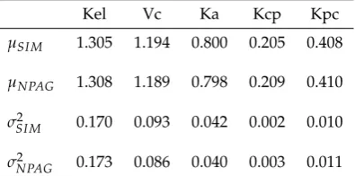
Table 1. Simulation versus optimization. Row 1: True simulated means for each parameter. Row 2: NPAG estimates of corresponding means. Row 3: True simulated variances for each parameter. Row 4: NPAG estimated variances for each parameter.
Kel Vc Ka Kcp Kpc
µSI M 1.305 1.194 0.800 0.205 0.408
µNPAG 1.308 1.189 0.798 0.209 0.410
σSI M2 0.170 0.093 0.042 0.002 0.010
σNPAG2 0.173 0.086 0.040 0.003 0.011
Twelve observations were taken at times 270
t=1.1, 5.4, 6.1, 6.5, 6.7, 7.8, 8.4, 9.2, 13.5, 15.3, 15.5, 15.8. 271
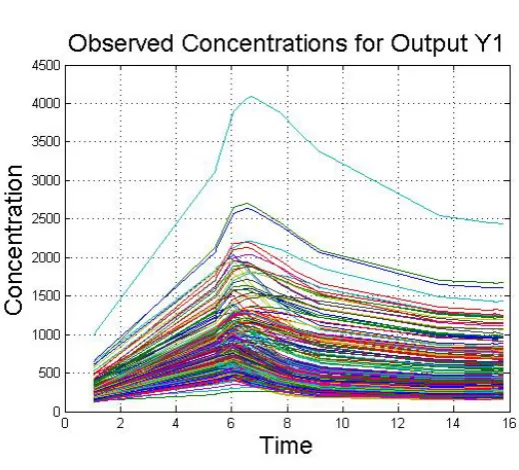
These sampling times were chosen in an ad hoc fashion and are not to be considered optimal. In Figure 272
2we show the profiles of the 300 noisy model outputsy1. These profiles are plotted as piecewise linear 273
functions with nodes at the observation times. 274
The initial Faure set had 80, 321 support points. After the first iteration of the NPAG algorithm, 275
the number of support points was down to 300, where it essentially stayed for the rest of the algorithm. 276
After 100 iterations NPAG was stopped based on the convergence criteria of Section 3.5. 277
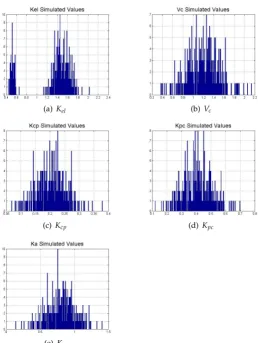
The simulated and estimated marginal distributions are shown in Figures3and4. It is seen that 278
the estimated marginal distributions were quite accurate. when compared to the simulated histograms. 279
In particular the bimodal shape ofKelwas uncovered. 280
NPAG is designed to estimate the whole joint distribution of the parameters. As mentioned earlier, 281
the estimateFMLis especially important for our application to population pharmacokinetics where 282
FMLis used as a prior distribution for Bayesian dosage regimen design. However,FMLis a consistent 283
estimator of the true mixing distribution and consequently, the moments ofFMLshould be consitent 284
estimators of the true moments. Means and variances of parameter estimates forFMLcan be easily 285
obtained by integrating the corresponding marginal distributions. So as a check of this fact, in Table1, 286
the comparisons of estimated versus simulated means and variances are shown. Again, results are 287
quite accurate, see Table1. 288
Finally, in Figure5we include a graph of Predicted versus Observed values which shows the all 289
around good fit of the data. The predicted values are gotten as follows: For each subject, the Bayesian 290
mean estimate of the parameters are found using the final NPAG distribution as a prior and that 291
subject’s observations. Then based on these parameter means, the subject’s concentration profile is 292
calculated. 293
4. Final Remarks and Conclusions
294
4.1. Final Remarks 295
The NPAG program was developed at the USC Laboratory of Applied Pharmacokinetics. James 296
Burke (University of Washington) developed the Primal-Dual Interior-Point method discussed in the 297
Appendix. Robert Leary (Pharsight Corporation) developed the Adaptive Grid method and wrote the 298
original Fortran program for NPAG. Michael Neely, MD (USC Children’s Hospital of Los Angeles) 299
developed the program package Pmetrics which contains NPAG as a subprogram. Pmetrics is an R 300
package for nonparametric and parametric population modeling and simulation and is available at 301
4.2. Conclusions 303
We have desribed a nonparametric maximum likelihood method called NPAG for estimating 304
multivariate mixing distributions. NPAG is based on an iterative algorithm employing the Primal-Dual 305
Interior-Point method and an Adaptive Grid method. Our method is able to handle high-dimensional 306
and complex mixture models. Other methods are discussed. A detailed description of NPAG is given. 307
The important application to population pharmacokinetics is described and a non-trivial example is 308
given. 309
In addition to population pharmacokinetics, this research also applies to empirical Bayes 310
estimation, see Koenker and Mizera [27] and to many other areas of applied mathematics, see Banks 311
et al.[28]. 312
Figure 1.Model.
Figure 2.True simulated model profiles.
Author Contributions: conceptualization, J.Burke, R.L and A.S.; data curation, M.v.G., M.N. and W.Y.; formal
313
analysis, J.Burke and A.S.; funding acquisition, J.Burke, R.J., M.N. investigation, M.N. and R.J.; methodology, R.L.,
314
T.T. and A.S., ; project administration, A.S.; resources, M.N. and R.J; software, M.v.G., A.K. and W.Y.; supervision,
315
A.S.; validation, J.Bartroff, D.B., J.Burke, A.K., R.L., T.T., A.S. and W.Y.; visualization, W.Y.; writing–original draft
316
preparation, W.Y.; writing–review and editing, J.Bartroff, D.B., J.Burke, A.K., R.L., T.T., A.S. and W.Y.
317
Funding:
318
This work was supported in part by grants from NIH: RR11526, GM65619, GM068968, EB005803, EB001978,
319
HD070886. JB was supported in part by NSF/DMS-0505712.
320
Conflicts of Interest:The authors declare no conflict of interest. The funders had no role in the design of the
321
study; in the collection, analyses, or interpretation of data; in the writing of the manuscript, or in the decision to
322
publish the results’.
323
Abbreviations
Algorithm 1NPAG Algorithm. Input: (Y,φ0,a,b,∆D,∆L,∆F,∆e,∆λ),aandbare the lists of lower
and upper bounds, respectively, ofΘ;∆Dis the minimum distance allowable between points in the estimatedFML.∆xsee §2.7. Output:(φ,λ,l(λ,φ)).
1: procedureNPAG(Y,φ0,a,b,∆D) .EstimateFMLgivenY
2: Initialization: φ = φ0, LogLike = −1030, F0 = 1030, F1 = 2∗F0, eps = 0.2, ∆e = 10−4, ∆F =10−2,∆L =10−4,∆λ =10
−3,n=0
3: whileeps≥∆eor|F1−F0| ≥∆F do
4: CalculateΨ(φ) .N×Kmatrix{p(Yi|φk)} 5: [λˆ(φ),l(λˆ(φ),φ)]←−PDIP(Ψ(φ)) .AppendixA
6: if (MAXCYCLES==0)then
7: FestML←−l(λˆ(φ),φ) 8: λ←−λˆ(φ)
9: return[φ,λ,FestML]
10: end if
11: n←−n+1
12: φc←−CONDENSE(φ,λˆ(φ),∆λ) .Alg. 3
13: [λˆ(φc),l(λˆ(φc),φc)]←−PDIP(Ψ(φc)) .PDIP returnsGn 14: NewLogLike=l(λˆ(φc),φc)
15: if (n>MAXCYCLES)then
16: FestML←−l(λˆ(φc),φc) 17: λ←−λˆ(φc)
18: return[φ,λ,FestML]
19: end if
20: if |NewLogLike−LogLike| ≤∆Landeps>∆ethen
21: eps=eps/2 .Adjust precision
22: end if
23: ifeps≤∆ethen .check EXIT conditions
24: F1=NewLogLike
25: if |F1−F0| ≤∆Fthen 26: FestML←−F1
27: φ←−φc;λ←−λˆ(φc)
28: return[φ,λ,FestML]
29: else
30: F0=F1;eps=0.2 .Reset Algorithm
31: end if
32: end if
33: φ←−φe←−EXPAND(φc,eps,a,b,∆D) .Alg. 2 34: LogLike←NewLogLike
35: end while
(a)Kel (b)Vc
(c)Kcp (d)Kpc
(e)Ka
Algorithm 2 EXPAND. Input: φ=(φ1,· · ·,φK), ∆G, Θ = [a1,b1]×[a2,b2]×...×[aQ,bQ], a = [a1,· · ·,aQ], b = [b1,· · ·,bQ], ∆D. Output: φ0=(φ01,· · ·,φ0M), where M ≤ K(1+2Q). Note: In
this algorithm,φ=(φ1,· · ·,φK)is aQ×Kmatrix, withQ=dimΘ.
functionEXPAND(φ,∆G,a,b,∆D)
2: Initialize:[Q,K] =size(φ),I=Q×QIdentity matrix, newφ←−φ
fork=1, ...,Kdo .K= number of input support points
4: ford=1, ...,Qdo .Q=dimΘ
T(d) =∆G(b(d)−a(d))
6: if φ(d,k) +T(d)≤b(d) then .Check upper boundary
φ+ =φ(:,k) +T(d)I(:,d) 8: dist=1030
end if
10: forkin=1 : length(newφ)do
newdist=∑abs(φ+−newφ(:,kin))./(b−a) .x ./y done component-wise 12: dist=min(dist, newdist)
end for
14: ifdist≥∆Dthen .Check distance to new support point newφ←−[newφ,φ+]
16: end if
ifφ(d,k)−T(d)≥a(d) then .Check lower boundary
18: φ− =φ(:,k)−T(d)I(:,d) dist=1030
20: end if
for kin=1 : length(newφ(1, :)) do
22: newdist=∑(abs(φ−−newφ(:,kin))./(b−a)) .x./y done component-wise dist=min(dist, newdist)
24: end for
ifdist≥∆Dthen .Check distance to new support point 26: newφ←−[newφ,φ−]
end if
28: end for
end for
30: φ←−newφ
end function
Algorithm 3Condense Algorithm. Input:(φ,λ,∆λ), Output:φcNote:φcis considered a subset ofφ
functionCONDENSE(φ,λ,∆λ)
ind=find(λ>(maxλ)∆λ) . Inequality and max are performed component-wise
φc=φ(:,ind)
returnφc
(a)Kel (b)Vc
(c)Kcp (d)Kpc
(e)Ka
Figure 4.Estimated Marginals of PK parameters.
The following abbreviations are used in this manuscript:
325
AG Adaptive Grid
ISDM Intrasimplex direction method
NPAG Nonparametric adaptive grid algorithm NPML Nonparametric maximum likelihood PDIP Primal-dual interior point method
QP Quadratic programming
Appendix A. A Primal-Dual Interior-Point Algorithm (PDIP)
327
To make this paper self-contained, we outline here the PDIP algorithm which was written by 328
James Burke. This algorithm is a FORTRAN subroutine of NPAG. The description below is based on 329
the Matlab and C++ codes found in Bradley Bell’s website, see [6]. Definition of general terms and 330
theorems can be found in Boyd and Vandenberghe [5]. 331
Appendix A.1. Duality Theory and the Basic Problem 332
Given a set of support points{φk}, the problem of finding the optimal weights{λk}in Eq.4can be posed as the following optimization problem
P minΦ(Ψλ) s.t. 0≤λ, e|λ=1,
whereΨ ∈ Rn×m is the matrix whose (i,j)entry is p(yi | φ
j) and where in general, the function Φ:Rk 7→R∪ {+∞}is given by
Φ(z) =
(
−∑k
i=1logzi , 0<z, and
+∞ , otherwise. (A1)
The symboleis always to be interpreted as the vector of all ones of the appropriate dimension. 333
The problemPis a convex programming problem since the objective functionΦis convex and the constraining region is a convex set. The Fenchel-Rockafellar dual of the convex programPis the problem
D minΦ(ω) s.t.L|ω≤me.
From Boyd we obtain the following Karush-Kuhn-Tucker (KKT) equations relating the solutions to the 334
problemPandD. 335
me=Ψ|w+y (A2)
e=WΨλ (A3)
0=ΛYe (A4)
where for any vectorx, we defineXto be the diagonal matrix havingxalong the diagonal. 336
Appendix A.2. An Interior-Point Path-Following Algorithm 337
The relaxed KKT is given by
me=Ψ|w+y (A5)
e=WΨλ (A6)
µe=ΛYe (A7)
0≤λ, 0≤w, 0≤y, (A8)
forµ>0. (µis the relaxation parameter.) A damped Newton’s method is used to solve the above
338
system. 339
Consider the functionF: R2m+n7→R2m+ngiven by
F(λ,w,y) =
Ψ|w+y WΨλ
ΛYe
A triple(λ,w,y)solves Eqs. A.A5to A.A8if and only if
F(λ,w,y) =
me e
µe
(A9)
and 0≤λ, 0≤ω, and 0≤y. Path-following algorithms attempt to solveA9by applying Newton’s method for progressively smaller values of the relaxation parameterµ. We first need the derivative of
F. It follows
F0(λ,ω,y) =
0 Ψ| I
WΨ Z 0
Y 0 Λ
wherez=Ψλ. 340
At the kth iteration of the algorithm, the Newton step is given by the solution to the nonsingular linear system
Fλk,wk,yk
+F0λk,wk,yk
∗hΛk,Wk,Yki|
=hem,en,µkem
i|
(A10)
whereyis constrained to satisfy the first KKT conditionyk=em−Ψ|wk. 341
The above set of equations can be reduced by standard techniques. It follows:
∆w=H−1r2 (A11)
∆y=−Ψ∆ω (A12)
∆λ=r1−λ−D1∆y (A13)
where H = D2−ΨD1Ψ|, D2 = ZW−1, D1 = ΛY−1,r1 = µY−1e, r2 = W−1e−Ψr1 where the 342
superscriptkis suppressed for simplicity. 343
Appendix A.3. The Algorithm 344
To describe the algorithm we need to define the variables: 345
q= m1 ∑mi=1λiyi 346
ρ=ke−W Zek∞
347
and the scaled duality gap 348
γ= |Φ1(ω)++|Φ(Ψλ)|Φ(Ψλ)|.
349
(Initialization) 350
Initially chooseλ0 = em/m,w0 = en/Ψλ0, andy0 = em−Ψ|w0. (Division of two vectors is 351
performed component-wise.) Setε=10−8.
352
(Iteration) 353
At iterationk+1, set 354
µk+1=σkqk
355
where the reduction factorσis defined by
σ= (
1 , ifµ≤εandρ>ε,
The next iterates are given byλk+1 =λk+δ1[∆λk],ωk+1 =ωk+δ2[∆ωk]andyk+1 =yk+δ2[∆yk], where the “damping” factorsδ1andδ2are defined by
δ1,0 =−
min(min(Λ−1∆λ),−1
2)
−1
δ2,0 =−
min(min(Y−1∆y), min(W−1∆w),−1
2)
−1
δ1=min(1, 0.99995δ1,0)
δ2=min(1, 0.99995δ2,0)
(Exit Conditions) 356
Iterate Eqs. A.11-A-13 until 357
µ≤εandρ≤εandγ≤ε.
358
If these conditions are not satisfied after a set number of iterations, then write “PDIP did not converge 359
in the given number of iterations.” 360
References
361
1. Kiefer, J.; Wofowitz, J. Consistency of the Maximum Likelihood Estimator in the Presence of Infinitely
362
many Incidental Parameters.Ann. Math. Statist.1956,27, 887–906.
363
2. Wang, X.; Wang, Y. Nonparametric multivariate density estimation using mixtures. Stat Comput2015,
364
25, 33–43.
365
3. Lindsay, B.G. The Geometry of Mixture Likelihoods: A general theory. Ann. Statist.1983,11, 86–94.
366
4. Mallet, A. A Maximum Likelihood Estimation Method for Random Coefficient Regression Models.
367
Biometrika1986,73, 645–656.
368
5. Boyd, S.; Vandenberghe, L.Convex Optimization; Cambridge UniversityPress, 2004.
369
6. Bell, B. Non-Parametric Population Analysis.
370
http://moby.ihme.washington.edu/bradbell/non_par/non_par.xml, 2012.
371
7. Baek, Y. An Interior Point Approach to Constrained Nonparametric Mixture Models. PhD dissertation,
372
University of Washington, Department of Mathematics, 2006.
373
8. Yamada, W.; Bartroff, J.; Bayard, D.; Burke, J.; van Guilder, M.; Jelliffe, R.; Leary, R.; Neely, M.; Kryshchenko,
374
A.; Schumitzky, A. The Nonparametric Adaptive Grid Algorithm for Population Pharmacokinetic
375
Modeling. Technical Report TR-2014-1, Children’s Hospital Los Angeles, Los Angeles, CA, 2014.
376
9. Fedorov, V.V.Theory of Optimal Experiments; Academic Press, 1972. edited and translated by W.J. Studden
377
and E.M. Klimko.
378
10. Schumitzky, A. Nonparametric EM Algorithms For Estimating Prior Distributions. Applied Mathematics 379
and Computation1991,45, 143–157.
380
11. Lesperance, M.L..; Kalbfleisch, J.D. An algorithm for computing the nonparametric MLE of a mixing
381
distribution. J. Am. Stat. Assoc.1992,87, 120–126.
382
12. Pilla, R.S.; Bartolucci, F.; Lindsay, B.G. Model building for semiparametric mixtures.arXiv2006.
383
13. Savic, R.M.; Kjellsson, M.C.; Karlsson, M.O. Evaluation of the nonparametric estimation method in
384
NONMEM VI.European Journal of Pharmaceutical Sciences2009,37, 27–35.
385
14. Savic, R.M.; Karlsson, M.O. Evaluation of an extended grid method for estimation using nonparametric
386
distributions.AAPS J2009,11, 615–627.
387
15. Leary, R. An overview of nonparametric estimation methods used in population analysis. Abstracts of the
388
Annual Meeting of the Population Approach Group in Europe; PAGE: Population Analysis Group Europe,
389
, 2017; Number Abstract 7383, p. 26.
390
16. Tatarinova, T.; Schumititzky, A. Nonlinear Mixture Models: A Bayesian Approach; Imperial College Press,
391
2015.
392
17. Jordan-Squire, C. Convex Optimization over Probability Measures. PhD dissertation, University of
393
Washington, Department of Mathematics, 2015.
18. Neely, M.; van Guilder, M.; Yamada, W.; Schumitzky, A.; Jelliffe, R. Accurate Detection of Outliers
395
and Subpopulations with Pmetrics: a non-parametric and parametric pharmacometric package for R.
396
Therapeutic Drug Monitoring2012,34, 467–476.
397
19. Faure, H. Discrépance de suites associées á un système de numération (en dimension s). Acta Arithmetica 398
1982,41, 337–351.
399
20. Bratley, P.; Fox, B.L. Algorithm 659: Implementing Sobol’s Quasirandom Sequence Generator. ACM 400
Transactions on Mathematical Software1988,14, 88–100. http://www.netlib.org/toms/659.
401
21. Fox, B.L. Algorithm 647: Implementation and Relative Efficiency of Quasirandom Sequence Generators.
402
ACM Transactions on Mathematical Software1986,12, 362–376. http://www.netlib.org/toms/647.
403
22. Davidian, M.; Giltinan, D.M.Nonlinear Models for Repeated Measurement Data; Chapman and Hall/CRC
404
Press, 1995.
405
23. Davidian, M.; Giltinan, D.M. Nonlinear Models for Repeated Measurement Data: An overview and update.
406
Journal of Agricultural, Biological, and Environmental Statistics2003,8, 387–419.
407
24. Ramos-Martin, V.; Johnson, A.; Livermore, J.; McEntee, L..; Goodwin, J.; Whalley, F..; Docobo-Perez, F.;
408
Felton, T.W.; Zhao, W.; Jacqz-Aigrain, E.; Sharland, M.; Turner, M.; Hope, W.W. Pharmacodynamics
409
of vancomycin for CoNS infection: experimental basis for optimal use of vancomycin in neonates. J 410
Antimicrob Chemother2016,71, 992–1002.
411
25. Drusano, G.; Neely, M.; van Guilder, M..; Schumitzky, A.; Brown, D.; Fikes, S..; Peloquin, C.; Louie, A.
412
Analysis of combination drug therapy to develop
413
regimens with shortened duration treatment for
414
tuberculosis. PLoS ONE2014,9, e101311.
415
26. Godfrey, K.R. The identifiability of parametric models used in biomedicine. Math Model1986,7, 1195–1214.
416
27. Koenker, R.; Mizera, I. Convex optimization, shape constraints, compound decisions, and empirical Bayes
417
rules. J. Am. Stat. Assoc.2014,109, 674–85. http://www.econ.uiuc.edu/$\sim$roger/research/ebayes/ 418
brown.pdf.
419
28. Banks, H.T.; Kenz, Z.R.; Thompson, W.C. A Review of Selected Techniques in Inverse Problem
420
Nonparametric Probability Distribution Estimation. Journal of Inverse and Ill-posed Problems 2012,
421
20, 429–460.