ABSTRACT
FU, HAIZHOU. Efficient, Effective, and Scalable Personalized Keyword Query Interpretation for RDF Databases. (Under the direction of Dr. Kemafor Anyanwu.)
The ease of use of the keyword search has made it an increasingly popular paradigm for querying (semi) structured data. Existing techniques supporting the keyword search are based on information retrieval (IR) paradigms. IR-style search paradigms follow a “semantics as match” style where objects containing keyword matches are returned as results that are not necessarily equivalent to the exact user-intended meaning of a query. Using such techniques leads to answer sets with heterogeneous semantics, leaving the user with the burden of sifting through the query results to identify the intended answers. Recent approaches supporting the keyword search incorporate an “interpretation” phase as part of the query-answering process. In the interpretation of keywords, the latter are mapped to structured constructs of queries. How-ever, keyword queries are often ambiguous because of their scanty and unstructured nature. Therefore, it is possible that there is no unique interpretation for a keyword query. Conse-quently, heuristics aimed to generate thetop-K most likely user-intended interpretations have been proposed. Unfortunately, the heuristics used by existing techniques often are not geared toward capturing user-dependent characteristics. Instead, they depend on database-dependent properties, such as the frequency of occurrence of database terms. This leads to the problem of generating interpretations that are not aligned with the intensions of users.
In this thesis we present an efficient, effective, and scalable context-aware keyword query in-terpretation system. The apex of this research framework includes the following three principal components:
of the current query. In other words, we can look at other older queries in the querying context to infer the intention of the current query. In this component, we incorporate query history as “inter-query context” to infer user intent. Major challenges that need to be addressed include how to represent query history as well as how heuristics based on such contextual information can be developed to bias the query interpretation process.
• Disambiguating Keyword Queries Using Intra-Query Context. A key part of mapping keywords to a structured query is identifying which sub-sequences of keywords are closely related, that is belong to the same mapping. We hypothesize that users write queries such that closely related keywords are clustered together as semantic units representing specific meanings. In other words, a keyword query is usually not a random permutation of words but consists of segments of related keywords. Consequently, the meaning of a keyword can be inferred from the “intra-query context” of neighboring keywords in the same segment. In this component, we tackle the problem of keyword querysegmentation to identify keyword segments.
c
Copyright 2014 by Haizhou Fu
Efficient, Effective, and Scalable Personalized Keyword Query Interpretation for RDF Databases
by Haizhou Fu
A dissertation submitted to the Graduate Faculty of North Carolina State University
in partial fulfillment of the requirements for the Degree of
Doctor of Philosophy
Computer Science
Raleigh, North Carolina
2014
APPROVED BY:
Dr. Rada Chirkova Dr. Munindar Singh
Dr. Nagiza Samatova Dr. Kemafor Anyanwu
BIOGRAPHY
ACKNOWLEDGEMENTS
First and foremost, I would like to thank my parents and my wife Fan Yang for their love, persistent support, motivation, guidance and inspiration throughout all my endeavors.
This work would not have been possible without the scientific advice and consistent mo-tivation of my supervisor and mentor Dr. Kemafor Anyanwu. I would like to thank her for the opportunities and the scientific guidance she gave me. Furthermore, I would like to thank my colleagues in the semantic computing research lab: Sidan Gao, Padmashree Ravindra and HeyongSik with whom I had many inspiring and fruitful scientific and philosophical discussions.
TABLE OF CONTENTS
LIST OF TABLES . . . vi
LIST OF FIGURES . . . vii
Chapter 1 Introduction . . . 1
1.1 Ambiguity in Keyword Query Interpretation . . . 5
1.2 Related Work . . . 6
1.2.1 Existing Solutions for The Keyword Search . . . 10
1.2.2 Existing Solutions for Personalized Search . . . 12
1.3 Key Components . . . 14
1.3.1 Component 1: Context-Aware Keyword Query Interpretation Using Inter-Query Context . . . 14
1.3.2 Component 2: Disambiguating Keyword Query Using Intra-Query Context 17 1.3.3 Component 3: Scaling Personalized Keyword Query Interpretation . . . . 19
Chapter 2 Context-Sensitive Keyword Query Interpretation Using Inter-Query Context . . . 23
2.1 Introduction . . . 23
2.2 Foundations and Problem Definition . . . 25
2.3 Representing Query History Using A Dynamic Cost Model . . . 32
2.4 Top-K Context-Aware Query Interpretation . . . 35
2.4.1 CoaGe . . . 35
2.4.2 Efficient Selection of Computing Top-k Combinations of Cursors . . . 38
2.5 Evaluation . . . 41
2.5.1 Effectiveness Evaluation . . . 42
2.5.2 Efficiency Evaluation . . . 45
2.6 Demonstration . . . 45
2.6.1 System Interface . . . 46
2.6.2 Demonstration Scenarios . . . 46
2.7 Related Work . . . 48
2.8 Conclusion . . . 50
Chapter 3 Disambiguating Keyword Query Using Intra-Query Context . . . . 51
3.1 Introduction . . . 51
3.2 Deep Segmentation . . . 55
3.3 Algorithm . . . 59
3.3.1 Computing Optimal Deep Segmentation . . . 59
3.3.2 Avoiding Graph Exploration (AGE) . . . 63
3.4 Evaluation . . . 65
3.4.1 Evaluation of Effectiveness . . . 66
3.4.3 Evaluation of Scalability . . . 68
3.5 Related Work . . . 69
3.6 Conclusion and Future Work . . . 70
Chapter 4 Scaling Personalized Keyword Query Interpretation . . . 73
4.1 Introduction . . . 73
4.2 Problem Definition . . . 76
4.3 Overview of Our Approach and System Architecture . . . 77
4.3.1 SKI System Architecture . . . 79
4.4 Keyword Query Interpretation in SKI . . . 81
4.4.1 Foundations . . . 81
4.4.2 Identifying Candidate Roots and Productive hits . . . 82
4.4.3 GeFree: A Graph Exploration Free Approach . . . 89
4.5 Evaluation . . . 92
4.5.1 Data, Query Scalability, and Performance . . . 93
4.5.2 Impact of Memory Consumption on Concurrency . . . 97
4.5.3 Impact of the Number of Slave Nodes on the Throughput . . . 98
4.5.4 Efficiency of Candidate Root Identification . . . 100
4.5.5 Other Factors that Impact the Performance of Free and Exploration-Based Query Interpretation Algorithms . . . 102
4.6 Related Work . . . 103
4.7 Conclusion . . . 104
Chapter 5 Conclusion . . . .105
LIST OF TABLES
Table 2.1 Complete cost model . . . 34 Table 2.2 Scenario B: Different contexts different rankings . . . 48 Table 2.3 Scenario C: The impact of length of query history on interpretation . . . . 48
LIST OF FIGURES
Figure 1.1 Example of keyword query interpretation . . . 4
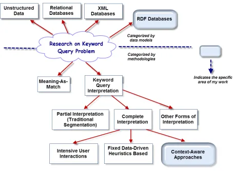
Figure 1.2 Taxonomy of research and the focus of this thesis . . . 7
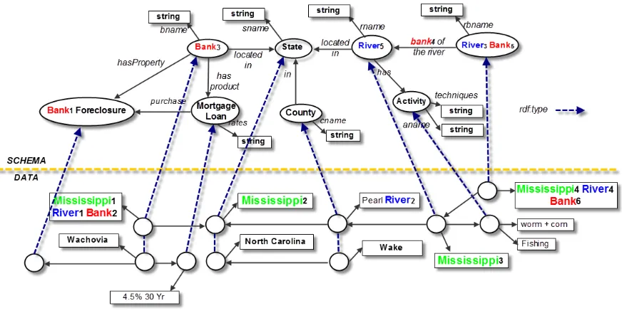
Figure 2.1 RDF schema and data graph . . . 24
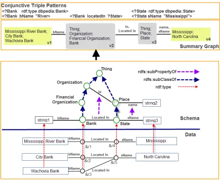
Figure 2.2 Graph summarization . . . 28
Figure 2.3 Architecture and workflow . . . 32
Figure 2.4 Efficiency and effectiveness evaluation . . . 42
Figure 2.5 Graphical user interface . . . 47
Figure 3.1 Different orderings of keywords lead to different semantics . . . 52
Figure 3.2 Pruning of not user-intended candidate interpretations by taking advan-tage of segmentation . . . 53
Figure 3.3 Pruning of more candidate interpretations by taking advantage of deep segmentation . . . 54
Figure 3.4 Example of RDF schema and data graph . . . 56
Figure 3.5 Example of shallow/deep segment and construction . . . 58
Figure 3.6 Examples of the matrix used for dynamic programming . . . 60
Figure 3.7 A running example . . . 62
Figure 3.8 Evaluation . . . 67
Figure 4.1 Architecture of SKI . . . 78
Figure 4.2 Architecture and workflow for a single slave node . . . 80
Figure 4.3 Example . . . 82
Figure 4.4 Group reachability bitmap index . . . 84
Figure 4.5 Question 2) How to identify nodes that can reach at least one node in all groups . . . 86
Figure 4.6 Example of path index . . . 90
Figure 4.7 Impact of query complexity on performance . . . 94
Figure 4.8 Performance of interpretation algorithms for same set of keyword queries on datasets with different scale . . . 95
Figure 4.9 Impact of MPL on latency . . . 96
Figure 4.10 Throughtput . . . 99
Figure 4.11 Efficiency evaluation: a) to f) . . . 101
Chapter 1
Introduction
institutions and so on. This is likely to become the dominant resource of structured knowledge on the Web. While there is also a standardized, structured query language for querying RDF data, called SPARQL[2], the complexity of such languages necessitates the development of easy-to-use query paradigms, such as the keyword search.
Earlier approaches to keyword searches on relational databases [3][5][41][23] considered the meanings of keywords as matches in the space of attribute values. This style is reminiscent of information retrieval (IR) paradigms where the meanings of keywords are also considered as matches in documents. However, this “meaning-as-match” style results in “shallow” query interpretations and therefore leads to poor quality results, which consist of a set of answers with heterogeneous semantics, so users have to sift through query results to identify most intended answers. For example, the IR-style search results of the keyword query “Jaguar Speed” would contain documents or entities related to “Jaguar” as animals or cars or aircrafts. Users have to check each item in the list of results to identify those results that match their intention. For example, the user only intends to find the “speed of jaguar as an animal.” The problem is more pronounced in RDF databases where data and metadata are queried simultaneously. In RDF databases, a keyword can play dual roles, that is as the label of an entity or a conceptual term. For instance, a keyword (e.g., “River”) could be interpreted as the attribute value of an entity, such as an address “765 River Bank Rd.” On the other hand, it can also be interpreted as a concept indicating “a large body of water,” where the results may not necessarily contain matches of keywords, such as “The Amazon” or “The Nile,” which will be missed in IR-style approaches.
There is a natural mapping from subgraphs to structured query components. Consequently, the role of each keyword needs to be interpreted, and the entire query needs to be mapped to a set of implied conditional expressions, such as the W HERE clause and the return clause. For example, a keyword query “Jaguar Speed” can be mapped to the following SPARQL query:
1.1
Ambiguity in Keyword Query Interpretation
Because keywords are ambiguous, usually there is more than one interpretation, that is, graph pattern of a keyword query. For example, “jaguar speed” can also be interpreted as “Find the animal jaguars and the average speed of them,” which can be represented by graph pattern B) in Figure 1.1, where “jaguar” hits the species property of the class node “:Animal” and “speed” hits the property “:avg speed” as shown in this figure. It is important to note that in this thesis the concept of the “ambiguity” of a particular keyword token represents different mappings from the data graph element that matches the keyword token to the schema graph elements, that is, classes or properties. This level of ambiguity is entirely different from counting the occurrences of keyword matches in the data graph level. Hence, a keyword that occurs several times in the data graph is not necessarily ambiguous if all of them can only be mapped to one class in the schema graph. For instance, in Figure 1.1, if “jaguar” only matches “JaguarXJ” and “JaguarXK,” it is not ambiguous because both are “Cars.” “Jaguar” is ambiguous only because another match of this keyword is mapped to “Animal,” an entirely different class in the schema graph.
impor-tant to capture and use information about the user’s current querying interests. User profiles are usually investigated to capture user-dependent properties. However, user profiles represent long-term search interests [60] [35] [40] [30]. For short-term interests, we focus on other queries, such as those a user or her friends asked recently. We also examine the queries themselves to provide contextual cues. There are extensive studies on the keyword search, keyword query interpretation, and personalized search. The related work is reviewed in the next sub-section.
1.2
Related Work
The keyword search has been extensively studied in unstructured, structured (relational databases) [3] [5] [23] [73] [72] [38] [64] [81], and semi-structured (XML [37] [76] [75] [77] [21] [83], RDF [13] [67] [68] [14] [16] [15]) databases. As illustrated in Figure 1.2, in terms of methodology, research on the keyword search can be generally categorized as the following: i) “meaning-as-match” (where keywords are only considered matches of documents or attribute values) and ii) keyword query interpretation (where an interpretation phase is incorporated before query executing). Traditional approaches to keyword segmentation provide only partial interpretation techniques. Moreover, for complete interpretation, the existing techniques are based on intensive user inter-actions or fixed data-driven methods, which cannot always generate high quality results. Our work focuses on incorporating context in a heuristics-based approach to improve the quality of keyword query interpretation. We will elaborate each branch of work in Figure 1.2 as follows.
Shallow Interpretation (“Meaning-as-match”)
Figure 1.2: Taxonomy of research and the focus of this thesis
matches. SPARK proposed a new simple but effective ranking formula by adopting existing IR techniques. BLINKS[20] showed a novel bi-level index that improved search efficiency. Since the indexing strategy needs a large amount of storage, a partition technique is introduced to partition the whole graph into several blocks based on the portal node, which is a cut node or separator in the graph. The indexes are built on both higher level blocks and inner-level blocks, which makes their backward search faster.
Complete Interpretation
use techniques that incorporate user input to incrementally construct queries by providing them with query templates. The limitation of these techniques is the extra burden they place on users.
Partial Interpretation
Other techniques [51][48][74][50] used to query relational databases offer some keyword query interpretation but to a lesser degree (i.e., partial interpretation). For example, keyword segmen-tation techniques identify segments of a keyword query. A valid segment should only contain a “valid” database term. However, to be able to generate a structured query from a keyword query, segments representing valid database terms can only be mapped to the conditional ex-pressions of structured formal queries. Other aspects of query interpretation, such as identifying which components are return expressions and how the different conditional expressions related to one another are not addressed by these techniques. Nevertheless, these techniques do not always identify the most relevant relationships between keywords, so the queries generated are not often the user intended ones.
queries are computed and mapped into the knowledge base. In contrast, instead of applying a probabilistic model, in this thesis we employ deterministic heuristics to infer user intended query structures. Gkorgkas et al. [17] proposed to interpret the intent of a keyword query after the answers are returned, which is entirely different from our approach because we interpret the intent before the query-answering phase. They extract features of keyword query results and classify the results based on similarities between querying results.
1.2.1 Existing Solutions for The Keyword Search
Keyword query interpretation takes place before query answering in the entire keyword query processing workflow. The general approaches used to generate top-K keyword query interpreta-tions over a schema graph are similar to most existing keyword search techniques. Approaches supporting the keyword search can be categorized into schema-based approaches and graph-based approaches.
Schema-based approaches. These approaches answer keyword queries by utilizing schema information to construct structured queries, such as SQL queries and SPARQL queries, accord-ing to the keywords in a keyword query. Two key steps are usually used to answer a keyword query using schema-based approaches in relational databases. In the first step, all candidate networks (CN)[23] are enumerated. In the second step, the candidate networks are evaluated to return a set ofminimal total joining network of tuples (MTJNT) [5][23]. However, because the number of M T J N T sis exponentially large, KRDBMS [52], DISCOVER-II [22], and SPARK [41][42] are approaches used to avoid enumerating all MTJNTs. However, the number of CNs increases exponentially with the size of the schema graph. Generating all CNs is inefficient even with proper pruning rules, especially in RDF databases with large schema graph. For more efficient query interpretation for RDF databases, CoSi [14][16] and Q2Semantics [68][67] introduce graph-based algorithms to identify top-K structured queries (i.e., SPARQL queries or conjunctive queries) progressively before answering the queries in RDF databases.
semi-structured or structured databases do not require the existence or assistance of a database schema. Those approaches aim at identifying subgraphs of the data graph that connects all keywords in a keyword query. According to the characteristics of the answers returned and the scoring functions used to rank the answers, the techniques can be grouped in three general categories:
I).Distinct Root Semantics (DRS). ForDRS, an answer to a keyword queryQis a sub-tree T of the data graphGD rooted atr∈V(GD), andT spans all keywords inQ. For any keyword nodevk∈T, there is an unique path betweenvk andrinT, denoted by< vk, r>T, which is the shortest path between them inGD. Hence, a rootrand a set of keyword nodes{vk1, vk2, ...vkm} uniquely identify an answerT to a keyword queryQ={k1, k2, ...km}. Therefore, given a set of keyword nodes, the search space of answer trees is O(n), where n=|V(GD)|; in other words, there are at mostndistinct roots and ndistinct answer trees. To answer queries with distinct root semantics, BLINKS [20] proposed a graph partitioning strategy and a shortest path based bi-level index to identify efficiently top-K answer trees with DRS. DPBF [12] proposed to the use of a best-first dynamic programming algorithm to find the optimal minimum Steiner tree. DPBF-k is a top-K algorithm of DPBF used to generate progressively approximate top-K Steiner trees rooted atk different nodes.
II). Steiner Tree Semantics (ST S). Compared with DRS, under ST S, an answer to a keyword query is also a treeT rooted atr ∈V(GD), andT spans all keywords in Q. However, the path between a keyword nodevkand the rootrdoes not have to be shortest path. Therefore, given a rootr and a set of keyword nodes{vk1, vk2, ...vkm}, the search space isO(m∆n), where
backward search to explore the graph from each keyword node. BANKS-II [27] improves upon BANKS by introducing a bidirectional expansion graph exploration algorithm.
III).Subgraph Semantics (SGS). Instead of the tree representation of answers, underSGS some approaches proposed returning subgraphs that span all keywords as answers. EASE [36] defined anr-radius Steiner graphas a subgraphGr ⊆GDthat spans all or a portion of keywords in Q where theradius of Gr is exactly r, and radius r is thecentric distance of the center of Gr, that is, the node with minimum centric distance. KRDBMS [52] proposed returning multi-centered subgraphs, in which each center and corresponding keyword nodes represent an answer under distinct root semantics. On the other hand, Ladwig et al. [33] argued that assuming a center of the answer graph restricts the search space. They introduce ad-length Steiner graph. In a d-length Steiner graph Gd, any keyword node vk has at least one other keyword node uk ∈V(Gd), such that the path betweenvk and uk inGd is of lengthdor less.
1.2.2 Existing Solutions for Personalized Search
derived from a user’s online reading or browsing activities. A mining algorithm is involved to re-rank the search results to achieve personalization. iii) Content-based personalization. Sopra et al. [10] took advantages of any available social information associated with Web content, such as tags, tweets, comments, rates, and they incorporated those social dimensions into the ranking function to personalize the search results. Shen et al. [57] proposed improving search quality by mining the long-term history of query logs. Query history has been utilized to dis-ambiguate and personalize keyword queries. However, in this thesis we propose to investigate short-term, user-specific query history. Compared with long-term history [61][44], short-term query history reflects the most recent search intentions. In addition, most query history-based personalization techniques are based on a query log containing all users’ search history. How-ever, in this work, we focus on utilizing the most recent query history of each individual user. Lee et al. [34] conducted a series of behavior experiments to argue that mining users’ Web search logs is effective in predicting users’ search intentions. Lee classified a user’s search goal into two groups. In the first group, users have specific goals in mind, and in the second group, users are expected to learn from the search on a particular topic. The results of the experiment show that human participants can classify accurately about 90 percent of the queries. iv) Social context-based personalization. Mohamed et al. [9] proposed adding a social context layer to the textual content traditionally used for indexing. The additional social context layer and the social index are fed into a query expansion module to achieve personalization.
1.3
Key Components
This research thesis consists of three components that improve the quality of keyword query interpretation in RDF databases by exploiting contextual information. There are two types of context: inter-query context andintra-query context. The inter-query context is represented by queries in the query history, and the intra-query context is represented by the latent substruc-tures of a keyword query (i.e., keyword segments and in the last component, solutions concerning performance enhancement, including efficiency and scalability) are discussed. The three key components of utilizing contextual information to improve the quality of the interpretation of keyword queries will be introduced in the following subsections.
1.3.1 Component 1: Context-Aware Keyword Query Interpretation Using Inter-Query Context
Research Challenges and Problems Solved: We observe that users are prone to issues a sequence of related queries. In this component we propose to take advantage of the query history to infer user intentions. There are three key challenges in the problem of generating the most likely user-intended keyword query interpretations by exploiting the query history as inter-query context. The problem solved in this component is called thecontext-aware keyword query interpretation problem, which includes the following challenging subproblems:
• Efficient representation scheme for query history as inter-query context. Query history
intent, which may not necessarily be the most frequent textual patterns. Our problem requires unstructured queries, their intended interpretations (structured queries), and the ontology to be managed and exploited. Whereas in IR tasks, the query and answer models are unstructured and require less sophisticated computational machinery such as indexes. More importantly, we designed a representation model, which is adynamic weighted graph model, to capture the evolving nature of the query history, and we developed a dynamic representation model.
• Develop heuristics to bias the selection of the most likely user intended candidate
inter-pretations. Existing approaches employ graph exploration algorithms, such as bidirec-tional search [27] or backward search [3], to identify subgraphs that connect the keyword matches. However, the heuristics employed in these approaches were developed to guaran-tee the compactness of the subgraphs. In other words, they are only efforts to make sure the keyword matches are closely connected in the data graph. To capture user-dependent characteristics, which are represented by the representation model, we incorporated the query history into the database-dependent heuristics, such that both the relevance of a keyword query to the user’ query interpretation history and the compactness of subgraphs are considered as two important factors to guide the graph exploration process.
• Improve the efficiency of the graph exploration algorithms. The graph exploration
reduce the search space of all combinations of paths, which impedes the efficiency. To overcome these challenges, we developed an efficient algorithm to solve the GST-K prob-lem, based on the dynamic representation model with maximum pruning of the search space.
Overview of Technical Solutions : This research introduces acontext-aware summary graph model to represent the database and the query history. The context-aware summary graph model is a dynamic weighted and labeled graph that summarizes the class subsumption hierarchy and the data graph. The context-aware summary graph model is associated with a context-aware cost model that assigns weights to the nodes and edges in the summary graph. The weights represent the relevance of the concepts indicated by the nodes or edges in the summary graph to the query history. The weights will be updated each time a user issues a new query. We further propose a context-aware graph exploration algorithm, which is an algorithm used to solve the GST-K problem over the context-aware summary graph. Unlike techniques [20][12] that can be applied to only static graphs, our approach does not require the pre-computation of paths, and therefore can be adapted to dynamic environments. The heuristics employed by the proposed algorithm i) prefer small subgraphs (semantically closely associated), ii) prefer subgraphs with minimum weights (the most relevant to the query history); and iii) grant priority to keyword matches that are most relevant to the query history. We also introduce a new early stopping condition to the graph exploration algorithm to reduce significantly the search space and improve efficiency. Chapter 2 describes this research and provides a performance evaluation of this model.
Major Contributions: In addressing the challenges of solving the context-aware keyword query interpretation problem, we make the followingcontributions:
i) Introduce and formalize the problem ofcontext-aware keyword query interpretation on RDF databases.
to capture concisely the essential characteristics of a user’s query history.
iii) Develop an efficient and effective top-K context-aware graph exploration algorithm that extends the existing cost-balanced graph exploration algorithms, with support for biasing the exploration process based on context as well as with early termination conditions based on a notion of dominance.
iv) Present a comprehensive evaluation of our approach using a subset of the DBPedia dataset.
1.3.2 Component 2: Disambiguating Keyword Query Using Intra-Query Context
Research Challenges and Problems Solved: We hypothesize that users write queries such that closely related keywords are clustered as a keyword segment in a keyword query. The user’s intended meaning of a particular keyword can be inferred from the context of the neighboring keywords in a keyword segment that contains this keyword. The second issue that we address in this thesis is the problem of generating the top-K most likely user-intended interpretation of keyword queries by exploiting the intra-query context captured by keyword segmentation. Two challenges are tackled in this component:
relationship of keywords in a keyword query and close semantic associations of keyword matches in the database cannot be limited to the keywords in the same database term. In contrast to such fine-grained segments, we identified coarser-grained keyword segments in the database to represent more general semantic units. We call this kind of segmentation “deep” segmentation.
• Find optimal deep segmentations. Because of the ambiguity of keyword queries, it is
possible that there are many different segmentations for a given keyword query. Different segmentations correspond to different user information needs. It is necessary to develop a ranking scheme to evaluate the quality of a deep segmentation. In addition, the search space of deep segmentations is larger than traditional segmentations because fine-grained segments are a subset of the coarser-grained segments. To solve this problem, we propose an efficient algorithm to identify the optimal deep segmentations.
Overview of Technical Solutions: Our second approach exploits the intra-query context as keyword segmentation to identify users’ search intent. We propose and formalize the concept of deep segmentation. We develop an algorithm that extends traditional “shallow” segmentation techniques by aligning the sub-sequences of keywords of a keyword query to as many closely related structured query constructs as possible. This means that we used the structure of the database as evidence for validating segmentations. A scoring function is developed to assess the quality of deep segmentations based on their structural characteristics. We propose a dynamic programming-based algorithm to find the optimal deep segmentations.
Major Contributions: We propose a “deep segmentation” technique for identifying the coarse-grained segments of a keyword query that correspond to logical semantic units that are typically ignored by existing techniques. Specifically, this paper makes the following contribu-tions:
techniques can. Furthermore, we formalize the problem of identifying the top-K interpre-tations of a keyword query by calculating its optimal deep segmeninterpre-tations using dynamic programming and a query-sensitive cost model.
ii) We present algorithms for computing deep segmentations and for top-K query interpre-tations that scale well for moderately sized schemas.
iii) We present extensive experimental results that show the effectiveness and performance of our approach in the context of significantly ambiguous queries, which previous studies have not considered.
1.3.3 Component 3: Scaling Personalized Keyword Query Interpretation Research Challenges and Problems Solved: The previous discussion of research issues regarding enabling context awareness for keyword query interpretation are all based on the assumption of a single-user, single-machine search environment. However, in practice a search system should also provide scalable solutions to support a multiuser environment. The exist-ing keyword query interpretation techniques are difficult to scale with the increasexist-ing number of users. The major reason is that keyword query interpretation techniques usually employ graph exploration-based algorithms, which suffer from high time and space complexity. The challenging research issues investigated, and resolved in this component include the following:
• Eliminate the overhead of graph exploration. For graph exploration-based algorithms,
with the same keyword query, under different query contexts, the probing sequences of paths can still be different. Some existing solutions have been proposed to pre-compute graph exploration states to avoid graph exploration. However, their approaches are either limited to much smaller search space requirements or cannot be applied to personalized interpretation techniques that use dynamic weighted graphs. That is because the over-head required by frequently updating the dynamic index is too costly. We tackled this problem by investigating a new indexing scheme such that in runtime the expensive graph exploration can be avoided.
• Improve concurrency. The high memory consumption of each instance of keyword query
interpretation is the bottleneck that impacts the concurrency. To maintain intermediate graph exploration search states for each query for a particular user, a memory of around 500 Mb is required to store the information in the dynamic weighted graph and inter-mediate graph exploration in a schema graph that includes around 1.3 million nodes and edges. Hence, for a server with 8G RAM, a maximum of only 17 user query requests can be processed concurrently. In order to allow more users to issue queries concurrently, we designed data structures that separate sharable user-independent information from dy-namic non-sharable user-dependent information and keep the non-sharable information to a minimum.
• Maximize throughput. First, the efficiency of every interpretation instance must be
Overview of Technical Solutions: In this component we design and implement a multi-tenant indexing scheme such that sharable graph exploration states for all users are pre-computed with reasonable memory consumption and non-sharable user-dependent information is kept to a minimum. The sharable graph exploration states include a set of pre-computed paths in the graph of lengths that are less than or equal to a specified threshold and a com-pressed bitmap group reachability index. The resulting interpretations can be generated by the fast identification of candidate roots and assembled using those pre-computed paths. The pro-posed interpretation algorithm eliminates the costly overhead required by graph exploration, particularly in achieving a personalized search, such that both the CPU time and memory usage are significantly reduced, therefore improving the concurrency in the multi-tenant envi-ronment over big data. To maximize the throughput, a distributed multi-tenant keyword query interpretation system is designed and implemented.
Major Contributions We propose an approach called “SKI” to meet the goal of scaling the concurrency of personalized keyword query interpretation over large scale data in multiuser environments. The SKI approach comprises the following:
i) A dual indexing scheme that captures user-specific information about concepts and re-lations that is the most relevant to a user’s current querying context and data-specific information about substructures in data. The former is captured in an index - personal-ized query context map (PCM) and the latter is captured in two key indexes, dense path index (DPI) - an index of subgraph structures and Rabit - a group reachability-based index. The data-specific indexes inform the decisions made by a graph exploration-free interpretation algorithm (GeFree) about which substructures to prune and how to as-semble substructures into complete interpretations. GeFree avoids the need for graph exploration, and it is fast and memory-efficient, thus reducing both latency and memory requirements of query interpretation.
weights associated with a user’s entry in the PCM. This ensures that the assembled in-terpretation is the most relevant to a specific user.
Chapter 2
Context-Sensitive Keyword Query
Interpretation Using Inter-Query
Context
2.1
Introduction
goal of identifying the K likeliest user intended interpretations.
Existing top-K query interpretation approaches [67] employed a cost-based graph explo-ration algorithm for exploring schema and data to find connections between keyword occur-rences and essentially fill in the gaps in a keyword query. However, these techniques have the limitation of using a “one-size-fits-all” approach that is not user-dependent but rather more database-dependent. Typically, the heuristics used are based on the presumption that the like-liest intended interpretation is the interpretation that has the most frequent support in the database. Unfortunately, since such metrics are not user-dependent, the results generated do not always reflect the user intent.
Figure 2.1: RDF schema and data graph
“Missis-sippi River Bank,” if a user had previously queried about “Mortgage Rates,” then it is more reasonable to select the interpretation of the current query as being that of a financial insti-tution “Mississippi River Bank.” On the other hand, if a user’s previous query was “Fishing Techniques,” it is more reasonable to interpret the current query as referring to a large body of water: the “Mississippi River.” Two main challenges that arise here include (i) effective capture and efficient representation of query history, and (ii) effective and efficient exploitation of query history during query interpretation. Towards addressing the challenges of solving the context-aware keyword query interpretation problem, we make the followingcontributions:
i) Introduce and formalize the problem ofContext-Aware keyword query interpretationon RDF databases.
ii) Propose a model and implementation of a Context-Aware summary graph model that is used to concisely capture essential characteristics of a user’s query history.
iii) An efficient and effective top-K Context-Aware graph exploration algorithm that extends existing cost-balanced graph exploration algorithms, with support for biasing the explo-ration process based on context as well as with early termination conditions based on a notion of dominance.
iv) It presents a Context-Aware graph exploration algorithm to compute a ranked list of K query interpretations.
v) we present a comprehensive evaluation of our approach using a subset of the DBPedia dataset.
2.2
Foundations and Problem Definition
represented by edge inED. An object node can either represent another entity (RDF resource) or literal value. λD is a labeling function λD : (VD ∪ED) → 2W that captures the rdfs:label declarations and returns a set of all distinct tokens in the label of any resource or property in the data graph. In addition, for any literal node vl∈VD, λD(vl) returns all distinct tokens in the literal value represented by vl. ϕD is the incidence function: ϕD :VD×VD →ED.
An RDF schema is also a collection of subject-property-object triples, which can also be represented as a graph: GS = (VS, ES, λS, ϕS, π), where the nodes in VS represent classes and edges in ES represent properties. λS is a labeling function λS :VS∪ES → 2W that captures the rdfs:label declarations and returns a set of all distinct tokens in the label of any class or property in the schema graph. ϕS is an incidence function: ϕS :VS×VS→ES. π:VS →2VD is a mapping function that captures the predefined property rdf:type maping a schema node representing a classC to a set of data graph nodes representing instances ofC. Nodes/edges in a schema can be organized in a subsumption hierarchy using predefined propertiesrdfs:subclass and rdfs:subproperty.
We define some special nodes and edges in the schema graph that are necessary for some of the following definitions:
• let VLIT ERAL ⊂VS be a set containing all literal type nodes (i.e., a set of literal nodes
representing literal types such as “XSD:string”);
• let VLEAF CLASS ⊆(VS−VLIT ERAL) be a set containing all leaf nodes (i.e. those nodes
representing classes who do not have sub-classes) who are not literal type nodes;
• letELEAF P ROP ERT Y ⊆ESbe a set containing all leaf edges (i.e. those edges representing
properties who do not have sub-properties);
• letVLEAF LIT ERAL⊆VLIT ERAL be a set containing all literal type nodes who are joined
with leaf edges, for example, in Figure 2.2, literal type nodevstring1 is inVLEAF LIT ERAL
butvstring2 is not because the edgeename connectingvP laceandvstring2 is not a leaf edge.
of which is selected from the alphabet W. Given a keyword query Q, an RDF schema and data graphs, the traditional problem that is addressed in relation to keyword queries on RDF databases is how to translate an keyword (unstructured) queryQinto a set of conjunctive triple patterns (structured query) that represents the intended meaning of Q. We call this process askeyword query “structurization”/interpretation. To ensure that the structured query has a defined semantics for the target database, the translation process is done on the basis of information from the data and schema graphs. For example, given a keyword query “Mississippi River Bank,” the schema graph and the data graph shown in Figure 2.2, we can find a structured query with conjunctive triple patterns listed at the top of Figure 2.2. Due to the class hierarchy defined in the schema, there could be many equivalent triple patterns for a given keyword query. For instance, in the schema graph of Figure 2.2, “Organization” is the super class of “Bank.” Assuming that only “Bank” has the property “bName,” thus, the two pattern queries:
h?x bName “river”i,h?x rdf:type Organizationi, and
h?x bName “river”i,h?x rdf:type Banki
are equivalent because the domain of the property “bName” requires that the matches of ?x can only be the instances of “Bank.” To avoid redundancy and improve the performance, usually a summary graph structure is adopted that concisely summarizes the relationships encoded in the subsumption hierarchies, and the relationships between tokens and the schema elements they are linked to.
Recall that our goal is to enable context-awareness for keyword query interpretation, we would also like this summary graph structure to encode information about a user’s query history such as which classes have been associated with recent queries. This leads to a notion of acontext-aware summary graph which is defined in terms of the concept of “Upward Closure”:
Figure 2.2: Graph summarization
e∧P is similarly defined.
Definition 2.2.2. (Context-aware Summary Graph) : Given an RDF schema graphGS, a data graph GD and a query history QH: QH={Q1, . . . , QT}, where QT is the most recent query, a context-aware summary graph can be defined as SG = (VSG, ESG, θ, λSG,ΨSG, ω), where
• θ:VSG∪ESG →2(VS∪ES) is an injective mapping function that maps any node or edge inSGto a set of nodes or edges in GS.
For example, the context-aware summary graph in Figure 2.2 contains{v1,v2,v3,v4} four nodes, each of which can be mapped to the upward closure of one of the leaf nodes in{vstring1,vBank,vState,vstring3} in the schema graph respectively.
• ESG ={ei|∃u∈ELEAF P ROP ERT Y such thatθ(ei) =u∧}.
For example, the summary graph in Figure 2.2 contains{e1,e2,e3}three edges, each of which can be mapped to the upward closure of one of the leaf edges in{ebN ame,elocatedIn, esN ame} respectively.
• λSG is a labeling function: λSG : (VSG∪ESG)→2W.
– ∀v∈VSG whereθ(v) =vC∧ and vC ∈VS representing classC, λSG(v) ={Svi∈vC∧λS(vi)} ∪ {
S
rj∈π(vC)λD(rj)},
i.e., union of all distinct tokens in the labels of the super classes of C and distinct tokens in labels of all instances ofC. For example, in Figure 2.2,
λSG(v4) ={ “Mississippi,” “North,” “Carolina”};
λSG(v3) ={ “Thing,” “Place,” “State”}.
– ∀e∈ESG where θ(e) =eP∧ and eP ∈ES representing propertyP, λSG(e) =Sei∈e∧PλS(ei),
which is a union of all distinct tokens in the labels of all super classes of P. For example,
λSG(e2) ={ “LocatedIn,”“ In”}.
• ΨSG is the incidence function: ΨSG :VSG×VSG→ESG such that ifθ(v1) =v∧C1, θ(v2) =
v∧C2, θ(e) =e∧P, then ΨSG(v1, v2) =eimpliesϕS(vC1, vC2) =eP.
Note that, we only consider user-defined properties for summary graph while excluding pre-defined properties. Further, we refer to any node or edge in a context-aware summary graph as a summary graph element.
Definition 2.2.3. (Hit): Given a context-aware summary graphSGand a keyword query Q, a hit of a keyword wi ∈ Q is a summary graph element m ∈ SG such that wi ∈ λ(m) i.e., wi appears in the label of m. Because there could be multiple hits for a single keyword w, we denote the set of all hits ofwasHIT(w). For example, in Figure 2.2,HIT(“bank”) ={v1, v2}.
Definition 2.2.4. (Keyword Query Interpretation): Given a keyword query Q and a context-aware summary graphSG, akeyword query interpretation QI is a connected subgraph of SGthat connects at least one hit of each keyword in Q.
For example, the summary graph shown in Figure 2.2 represents the interpretation of the keyword query “Mississippi, River, Bank” which means “Returning those banks in the Mis-sissippi State whose name contains the keyword ’River’ .” The equivalent conjunctive triple patterns are also shown at the top of Figure 2.2. Note that for a given keyword queryQ, there could be many query interpretations due to all possible combinations of hits of all keywords. Therefore, it is necessary to find a way to rank these different interpretations based on a cost function that optimizes some criteria which captures relevance. We use a fairly intuitive cost function in the following way: cost(QI) =P
mi∈QIω(mi),
which defines the cost of an interpretation as a combination function of the weights of the elements that constitute the interpretation. We can formalize thecontext-aware top-k keyword query interpretation problem as follows:
(i.) QIi∈T OP K and QIj ∈([[Q]]−T OP K), cost(QIi)≤cost(QIj). (ii.) If 1≤p < q ≤k,cost(QIp)≤cost(QIq), whereQIp, QIq∈T OP K.
This problem is different from the traditional top-k keyword query interpretation problem in that the weights are dynamic and are subject to the evolving context of query history. Because some queries are more ambiguous than others, keyword query interpretation problem requires effective techniques to deal with large interpretation space. We propose a concept calledDegree of Ambiguity (DoA) for characterizing the ambiguity of queries: The DoA of the keyword queryQis defined asDoA(Q) =Q
wi∈Q|HIT(wi)|, which is the number of all combinations of
keyword matches. It will be used as a performance metric in our evaluation.
Overview of our approach. Having defined the problem, we start with an overview of our approach. It consists of the following key steps as shown in Figure 4.3:
• Find keyword hits using an inverted index for a given keyword query Q. (Step (1)–(3)).
• The query interpreter takes the hits and utilize a graph exploration algorithm to generate
a set of top-K interpretations ofQ. (Step (4)–(5))
• The top-1 interpretation of the top-K interpretation is passed to a cost model to update
the weights of the context-aware summary graph. (Step (6)–(7))
• Steps involved in Figure 4.3 only capture one of the iteration cycles of the interactions
between user and our interpretation system. The new weights of context-aware summary graph will be used to bias the graph exploration in the next iteration when user issues a new query
Figure 2.3: Architecture and workflow
2.3
Representing Query History Using A Dynamic Cost Model
To achieve this effect, we designed the dynamic weighting function to be based on arelevance function in terms of two factors: historical impact factor (hif) and region factor (rf).
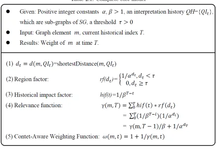
LetT indicate the historical index of the most recent queryQT,tbe the historical index of an older keyword query Qt, i.e., t≤T, and m denote a summary graph element. Assume that the top-1 interpretation for Qthas already been generated : QIt. Region factor is defined as a monotonically decreasing function of the graph distanced(m, QIt) betweenm and QIt:
rf(d(m, QIt)) = αd(m,QIt1 )
(rf(d(m, QIt)) = 0if d(m, QIt) ≥τ) τ is a constant value, and d(m, QIt) is the shortest distance between m and QIt, i.e., among all the paths from m to ANY graph element in the subgraphQIt,d(m, QIt) is the length of the shortest path. α >1 is a positive integer constant. The region factor represents the relevance of m to QIt. Historical impact factor captures the property that the relevance between a query and a graph element will decrease when that query ages out of the query history. hif is a monotonically decreasing function: hif(t) = 1/βT−t, where β > 1 is also a positive integer constant. We combine the two factors to define the relevance ofm to query interpretationQIt ashif(t)∗rf(d(m, QIt)). To capture the aggregate historical and region impacts of all queries in a user’s query history, we use the combination function as the relevance functionγ :
γ(m, T) =XT
0 hif(t)∗rf(d(m, QIt)) = XT
0 (1/β
T−t)(1/αd(m,QIt)) (2.1)
To produce a representation of (1) for a more efficient implementation, we rewrite a function as recursive:
γ(m, T) =γ(m, T −1)/β+ 1/αd(m,QIT) (2.2)
The consequence of this is that, given the relevance score of m at time T −1, we can calculate γ(m, T) simply by dividing γ(m, T −1) by β then adding 1/αd(m,QIT). In practice,
have their scores updated.
Boostrapping. At the initial stage, there are no queries in the query history, so the relevance score of the summary graph elements can be assigned based on the T F −IDF score, where each set of labels of a summary graph element m i.e., λSG(m) is considered as a document. User-feedback is allowed at every stage to select the correct interpretation if the top-1 query interpretation generated is not the desired one.
Table 2.1: Complete cost model
ω(m, t) = 1 + 1/γ(m, t) (2.3)
This implies that a summary graph element with a higher relevance value will be assigned a lower weight. The complete cost model is shown in Table 2.1. In the next section we will discuss how to find interpretations with top-k minimal costs.
2.4
Top-K Context-Aware Query Interpretation
The state of the art technique for query interpretation uses cost-balanced graph exploration algorithms [67]. Our approach extends such an algorithm [67] with a novel context-aware heuristic for biasing graph exploration. In addition, our approach improves the performance of the existing algorithm by introducing an early termination strategy and early duplicate detection technique to eliminate the need for duplicate detection as a postprocessing step. Context Aware Graph Exploration (CoaGe) algorithm shown in Algorithm 1.
2.4.1 CoaGe
Algorithm 1 CoaGe
1: Input: Initialize priority queuesT OP K,CQ.
2: Create cursor for each hit of each keyword;
3: Insert each cursor toCQ;
4: whileCQ is not emptydo
5: c=CQ.ExtractM in(); //get cheapest cursor
6: v=cursor.path[0]; //the visiting node
7: if v is a rootthenT opKCombination(T OP K, v.CL)
8: if T OP K.count≥K∧T OP K.M ax()< CQ.M in() then
9: TERMINATE;
10: end if
11: end if
12: if c.depthis less than the threshold then
13: for allneighborn ofv do
14: if nis not visited by cthen
15: create new cursornew cursor forn;
16: if c.topN ==F ALSE then
17: c.cost∗=penalty factor;
18: end if
19: n.CL[c.keyword].Add(new cur);
20: end if
21: end for
22: end if
Each node v in the context-aware summary graph has a cursor manager CL that contains a set of lists. Each list in CL is a sorted list that contains a sequence of cursors for keyword w that have visited v, we use CL[w] to identify the list of cursors for keyword w. The order of the elements in each list is dependent on the costs of cursors in that list. The number of lists inCL is equal to the number of keywords: |CL|=|Q|.During the graph exploration, the cursor with minimal cost is extracted from CQ(line 5). Let v be the node just visited by this “cheapest” cursor (line 6). CoaGefirst determines whether vis a root (line 7). This is achieved by examining if all lists in v.CL is not empty, in other word, at least one cursor for every keyword has visitedv. Ifv is a root, then, there areQ
wi∈Q|v.CL[wi]|combinations of cursors.
Each combination of cursors can be used to generate a subgraphQI. However, computing all combinations of cursors as the traditional approach [67] does is very expensive. To avoid this, we developed an algorithm T opCombinationto enable early termination during the process of enumerating all combinations. T opCombination algorithm (line 7) will be elaborated in the next subsection. A second termination condition for theCoaGealgorithm is if the smallest cost of CQis larger than the largest cost of the top-K interpretations (line 8). After the algorithm checks ifvis a root or not, the current cursorcexplores the neighbors ofvif the length ofc.path is less than a threshold (line 12). New cursors are generated (line 15) for unvisited neighbors of c (not in c.path, line 14). New cursors will be added to the cursor manager CL of v (line 19). The cost of new cursors are computed based on the cost of the path and ifc is originated from a top-N hits.
and cA.cost∗penalty f actor > cB.cost. The space complexity is bounded byO(n·dD), where n=P
wi∈Q|HIT(wi)|is the total number of keyword hits,d= ∆(SG) is the maximum degree
of the graph, and Dis the maximum depth a cursor can explore.
2.4.2 Efficient Selection of Computing Top-k Combinations of Cursors
Algorithm 2 Pseudocodes for TopKcombination algorithm
1: Initialize the combination enumeratorEnum=CL.CEnum.
2: Initialize the threshold listT L;
3: whilecur comb=Enum.current()∧cur comb! =N U LL do
4: if ∃h∈T L,Dominate(cur comb, h) ==T RU E then
5: if Enum.DirectN ext(h) ==N U LLthen
6: break;
7: end if
8: else
9: if DuplicateDetection(cur comb, T OP K) ==T RU E then
10: if Enum.Next() ==N U LLthen
11: break;
12: else
13: continue;
14: end if
15: else
16: //not a duplicate combination
17: if T OP K.count≥K∧T OP K.M ax()< cur comb.cost then
18: T L.Add(cur comb);
19: if Enum.DirectNext(v) ==N U LL thenbreak;
20: end if
21: else
22: if T OP K.count≥K then
23: T OP K.ExtractM in();
24: T OP K.Insert(cur comb);
25: end if
26: if Enum.Next() ==N U LL thenbreak;
27: end if
28: end if
29: end if
30: end if
The T opCombination algorithm is used to compute the top-K combinations of cursors in the cursor manager CL of a node v when v is a root. This algorithm avoids the enu-meration of all combinations of cursors by utilizing a notion of dominance between the ele-ments of CL. The dominance relationship between two combinations of cursors Comp = (CL[w1][p1], ...CL[wL][pL]), andComq= (CL[w1][q1], ...CL[wL][qL]) is defined as follows: Comp
dominates Comq, denoted by Comp Comq if for all 1 ≤ i ≤ L = |Q|, pi ≥ qi, and exists 1≤j≤L,pj > qj. Because every listCL[wi]∈CLis sorted in a non decreasing order, i.e., for all 1≤s≤L,i≥jimplies thatCL[ws][i].cost≥CL[ws][j].cost. Moreover, because the scoring function for calculating the cost of a combination Comis a monotonic function: cost(Com) =
P
ci∈Comci.cost, which equals to the sum of the costs of all cursors in a combination, then we
have:
Comp= (CL[w1][p1], CL[w2][p2], ..., CL[wL][pL])
(Comq=CL[w1][q1], CL[w2][q2], ..., CL[wL][qL])
implies that for all 1≤i≤L,
CL[wi][pi].cost≥CL[wi][qi].cost andcost(Comp)≥cost(Comq).
In order to compute top-K minimal combinations, given the combinationCommaxwith the max cost in the top-K combinations, we can ignore all the other combinations that dominate Commax. Note that, instead of identifying all non-dominated combinations as in line with the traditional formulation, our goal is to find top-K minimum combinations that require dominated combinations to be exploited.
Com0= (CL[w1][0], CL[w2][0], ..., CL[wL][0]), which is the “cheapest” combination in CL. Let
Comlast = (CL[w1][l1], CL[w2][l2], ..., CL[wL][lL]), be the last combination, which is the
most “expensive” combination and li =CL[wi].length−1, which is the last index of the list CL[wi].
The enumerator outputs the next combination in the following way: if the current combi-nation is
Comcurrent= (CL[w1][s1], CL[w2][s2], ..., CL[wL][sL]),
from 1 toL,Enum.N ext() locates the first indexi, where 1≤i≤Lsuch thatsi≤li, and returns the next combination as Comnext =
(CL[w1][0], ..., CL[wi−1][0], CL[wi][si+ 1], ..., CL[wL][sL]),
where, for all 1 ≤j < i,sj is changed from lj−1 to 0, and sj =sj+ 1. For example, for (CL[w1][9], CL[w2][5]), if CL[w1].length equals to 10 and CL[w2].length > 5, then, the next
combination is (CL[w1][0], CL[w2][6]). The enumerator will terminate when Comcurrent ==
Comlast.
Each time Enum move to a new combination curcomb, it is compared with every combi-nation inT L to check if there exists a threshold combinationh ∈T L such that cur combh (line 4). If so, instead of moving to the next combination using N ext(), Enum.DirectN ext() is executed (line 5) to directly return the next combination that does not dominate h and has not been not enumerated before. This is achieved by the following steps: if the threshold combination is
Comthreshold= (CL[w1][s1], CL[w2][s2], ..., CL[wL][sL]),
from 1 to L, Enum.DirectN ext() locates the first index i, where 1 ≤ i ≤ L such that si 6= 0, and from i+ 1 to L,j is the first index such thatsj 6=lj−1, then the next generated combination is Comdirect next=
comthreshold= (CL[w1][0], CL[w2][6], CL[w3][9], CL[w4][2]),
assume that the length of each list in CL is 10, then its next combination that does not dominate it is
comdirect next= (CL[w1][0], CL[w2][0], CL[w3][0], CL[w5][3]).
In this way, some combinations that could be enumerated by “Next()” function and will dominate comthreshold will be ignored. For instance,comnext =N ext(comthreshold) =
(CL[w1][1], CL[w2][6], CL[w3][9], CL[w4][2]),
and the next combination after this one: N ext(comnext) = (CL[w1][2], CL[w2][6], CL[w3][9], CL[w4][2])
will all be ignored because they dominate comcurrent.
If a new combination is “cheaper” than the max combination inT OP K, it will be inserted to it (line 24), otherwise, this new combination will be considered a new threshold combination, and inserted toT L(line 18) such that all the other combinations that dominate this threshold combination will not be enumerated. The time complexity of T opKCombination is O(Kk), where K =|T OP K|is the size of T OP K,k =|Q|is the number keywords. Because, for any combination
com= (CL[w1][s1], ..., CL[wL][sL]), where for allsi, 1≤i≤L,si≤K comK = (CL[w1][K+ 1], ..., CL[wL][K+ 1])com
In the worst case, any combinations that dominatescomK will be ignored andKk combina-tions are enumerated. Consequently, the time complexity ofCoaGe isO(n·dD ·Kk), wheren is the total number of keyword hits,d= ∆(SG) is the maximum degree of the graph, Dis the maximum depth. The time complexity of the approach in [67] (we call this approach T KQ2S) isO(n·dD·SD−1), where S=|SG|is the number of nodes in the graph.
2.5
Evaluation
Figure 2.4: Efficiency and effectiveness evaluation
running on Windows 7 Professional. Our test bed includes a real life dataset DBPedia, which includes 259 classes and over 1200 properties. We will compare the efficiency and effectiveness withT KQ2S.
2.5.1 Effectiveness Evaluation
evaluators we did not use more than 10 groups in this questionnaire). Each group contains a short query log consisting of a sequence of up to 5 keyword queries from the oldest one to the newest one. For each group, the questionnaire provides English interpretations for each of the older queries. For the newest query, a list of candidate English interpretation for it is given, each interpretation is the English interpretation representing a structured query generated by either T KQ2S or CoaGe. Therefore, this candidate interpretation list provided to user is a union of the results returned by the two algorithm. Then users are required to pick up to 2 interpretations that they think are the most intended meaning of the newest keyword query in the context of the provided query history. A consensus interpretation (the one that most people pick) was chosen as the desired interpretation for each keyword query. (Sample queries, questionnaires, experimental results and the statistics of the user feedback can be found from the following link: http://research.csc.ncsu.edu/coul/experiments.rar.)
Metrics. Our choice of a metric of evaluating the query interpretations is to evaluate how relevant the top-K interpretations generated by an approach is to the desired interpretation. Further, it evaluates the quality of the ranking of the interpretations with respect to their relative relevance to the desired interpretation. Specifically, we adopt a standard evaluation metric in IR called “Discounted cumulative gain (DCG)” with a refined relevance function: DCGK =
K
P
i=1
2reli−1
log2(1+i), where K is the number of top-K interpretations generated, and reli is the graded relevance of the resultant interpretation ranked at position i. In IR, the relevance between a keyword and a document is indicated as either a match or not,reli is either zero or one. In this research the relevance between a resultant interpretationQI and a desired inter-pretationQID for a given keyword query Q cannot be simply characterized as either a match or not. QI and QID are both subgraphs of the summary graph and could have some degree of overlapping, which means reli ∈ [0,1]. Of course, if QI == QID, QI should be a perfect match. In this experiment, we define the relevance between a candidate interpretationQI and the desired interpretation QID as: reli =
|QIi∪QID|−|QIi∩QID|
|QIi∪QID| , where QIi is the interpretation
the union of the the two subgraphs. Large overlapping implies high similarity betweenQIi and QID, and therefore, high relevance score. For example, ifQIi has 3 graph elements representing a class “Person,” a property “given name” and a class “XSD:string.” The desired interpretation QID also has 3 graph elements, and it represents class “Person,” a property “age” and a class “XSD:int.” Therefore, the relevance between QIi and QID is equal to 1/5 = 0.2 because the union of them contains 5 graph elements and they have 1 common node.
On the other hand, we use another metric precision to evaluate the results. The precision of a list of top-K candidate interpretation is:
P@K =|relevant interpretations inT OP K|/|T OP K|,
which is the proportion of the relevant interpretations that are generated inT OP K. Because sometimes, when the user votes are evenly distributed, the consensus interpretation cannot represent the most user intended answer, our evaluation based onDCGmay not be convincing. The precision metric can overcome this limitation by consider the candidate interpretations that over 10% people have selected as desired interpretations.
the ith group contains all the queries in the (i−1)th group plus a new query. Given the 4 different query histories, the two algorithms are to interpret another query Q. (c) illustrates the quality of interpretingQgiven different query histories. We can observe that our approach will do better with long query history. But for the first group, both algorithms generate a set of interpretations that are very similar to each other. Both the DCGvalues are high because user have to select from the candidate list as the desired interpretation, even though they may think none of them is desired. For the third group, that difference in performance is due to a transition in context in the query log. Here the context of query changed in the 2nd or 3rd query. This resulted in a lower DCG value which started to increase again as more queries about new context were added.
2.5.2 Efficiency Evaluation
From the result of the efficiency evaluation in Figure 2.4 (d)–(f), we can see that, our algo-rithm outperforms T KQ2S especially when the depth (maximum length of path a cursor will explore) and the number of top-K interpretations and the degree of ambiguity DoA is high. The performance gain is due to the reduced search space enabled by early termination.
2.6
Demonstration
2.6.1 System Interface
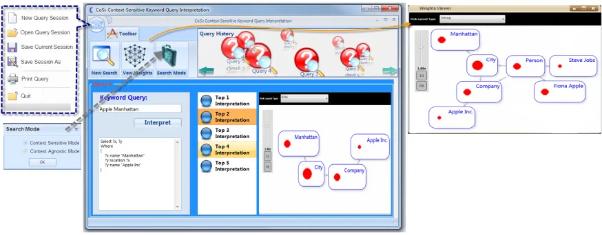
Figure 2.5 shows the graphical user interface. By default, CoSi enables a context-sensitive interpretation mode. Users can also manually change the mode by clicking the “Search Mode” button. The users can start a new session by choosing “New Query Session” on the menu. By clicking the “New Search” button, user can start issuing keyword queries and browse the results. After user click the “Interpret” button, the system will generate a ranked list of up to five candidate interpretations. By selecting one of the candidate interpretations, the corresponding SPARQL query will be shown in the text box under the “Interpret” button. Users can also view any interpretation from the list and a subgraph that is equivalent to the interpretation of the keyword query will be shown on a panel in the main interface. Any information related to issued queries such as keywords, candidate interpretations (subgraphs and SPARQL queries) will be recorded. User can select to view the information of any query in the query history by clicking that query in the list shown on the top-right carousel panel control. The entire history of query interpretations can be saved by using the “Save Query Session” function on the main menu. CoSi also provides users a “weights viewer” to see the subgraph of the weighted summary graph. The size of the red circle in the node reflects the value of the weight. The subgraph contains nodes and edges related to all the queries in the query history. The users can observe the changes of subgraphs caused by the evolving context. Finally, the end users can choose to investigate the results of using context-agnostic mode, where the traditional approach is applied.
2.6.2 Demonstration Scenarios
The results of the demonstration of the CoSi system show some interesting features. Three interesting user cases are given:
Figure 2.5: Graphical user interface
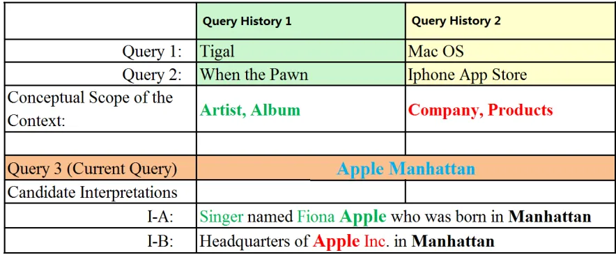
Scenario B: ScenarioB shown in Table 2.2 illustrates a more interesting feature of CoSi. Given a keyword query “Apple Manhattan,” assume that two possible interpretations areI−A and I −B. Given two different query histories (The end users can load existing query logs by clicking “open query session” from the main menu), CoSi ranks I −A higher by loading “Query History 1” because the conceptual scope of this search session is about “artist” and “album.” Alike, CoSi ranks I−B higher if “Query History 2” is loaded because the context is all about “company” and “products.” Therefore, CoSi can detect the context which reflects the users’ focus and interests during the specific query session, while traditional methods (using context-agnostic mode) will always return the same ranking regardless of the context.
Table 2.2: Scenario B: Different contexts different rankings
Table 2.3: Scenario C: The impact of length of query history on interpretation
But traditional interpretation systems are not helpful because they are not context-sensitive. Users still need to sift through the search results. But with CoSi, when people search in an exploratory way by issuing serial queries, CoSi will learn what they are really asking for and rank the intended interpretation higher such that the end users can find them more easily.
2.7
Related Work
address the query interpretation problem partially. STAR [28] proposed an efficient approximate Minimum Steiner Tree algorithm to compute top-K optimal connecting trees. However, the problem addressed in this problem is more related to the Group Steiner Tree problem, which can be addressed using that technique. BLINKS [20], proposed a novel bi-level indexing strategy based on graph partitioning that improves the efficiency of graph exploration. However, its indexing is targeted at a statically weighted graph which to be adapted for our purposes will require re-indexing after every query.
2.8
Conclusion
Chapter 3
Disambiguating Keyword Query
Using Intra-Query Context
3.1
Introduction
In Chapter 1, we discussed the general approach of keyword query interpretation used by current techniques, which are attempts to find the “best” subgraphs (of the schema plus data graph) that connect a set of keywords given in the query. These top subgraphs are supposed to represent the likeliest intended interpretations which can then be translated to structured queries in a straightforward way. The graph exploration algorithms for computing the subgraphs rely on fixed data-driven heuristic measures that allow converge on the “best” subgraphs early. The approach introduced in Chapter 2 provides a solution based on query history to overcome the limitation, where traditional approaches cannot always generate the most user-intended interpretations.
Figure 3.1: Different orderings of keywords lead to different semantics
words (as in the “bag-of-words” view), but rather a set of logical word groupings. Each group represents a set of terms that are intended to have close associations in the knowledge base, we call each such group asemantic unit or keyword segment. For example, in Figure 3.1, given a set of words “Mississippi,” “River,” and “Bank,” the query “River Bank Mississippi” are more likely intended to mean “River banks located in Mississippi state” according to the knowledge base. On the other hand, the query “Bank Mississippi River” using the same set of words has a more likely intended meaning as, “Name of a bank as Mississippi river,” We can see that the difference between the earlier query, and the latter one is that in the earlier query, the intension of the concept of River Bank is reflected in the query, which places them close to each other in the query and also close in the knowledge base (representing a class name). In the other query, however, “Mississippi River” is more closely related in both query and the knowledge base. Consequently, it may be possible to more accurately capture the intended semantic units in a query using a “set of keyword sub-sequences,” where the keyword sub-sequence represents any associations suggested by the user query and the knowledge base.