Design, Modeling, and Control of a Variable Geometry Spray Fuel Injector.

(1)

ABSTRACT

LIEN, JOHN PAUL. Design, Modeling, and Control of a Variable Geometry Spray Fuel Injector. (Under the direction of Gregory D. Buckner.)

This dissertation describes the design of a variable geometry spray fuel injector. The

injector is expected to enable advanced combustion modes by allowing the geometry of

the injected spray (specifically the internal angle of its hollow cone) to vary throughout

the intake and compression strokes, thereby enabling optimal targeting of fuel.

An eternally-opening pintle-type injector nozzle has been designed and shown, through

experimental testing, to meet the requirements of a VGS injector. Spray angles from

20-150 degrees are achieved with pressurized (100 bar) iso-octane in open air. Droplet sizes

within the spray are measured using laser diffraction and found to be smaller than 50µm

Sauter Mean Diameter at most spray angles.

A piezoelectric (PZT) actuation system has been developed to position the pintle

elec-tromechanically. To enable model-based control of the actuator, a novel, high-fidelity,

computationally efficient model for the non-linear, hysteretic behavior of PZT was

de-veloped and experimentally validated. The model is based on a class of neural networks,

called Hysteretic Recurrent Neural Networks, which mimic the electromechanical

char-acteristics of PZT. Training techniques based on Bayesian inference, genetic algorithms,

and (Levenberg-Marquardt) least-squares optimization are developed for the model and

their performance is compared to other modeling techniques (such as Radial Basis

Func-tion Networks and the threshold-discrete Prandtl-Ishlinskii Model) on experimental data.

It is shown that the HRNN model exhibits superior generalization capabilities to both

of those models.

(2)

error along a realistic spray angle trajectory. The controller pre-computes a feed-forward

optimal input command offline, which is supplemented with PI feedback at runtime. This

controller is shown to be superior to pure PI control in experimental tests, and offers much

simpler implementation than typical optimal control schemes. To implement feedback

control without external sensing, a model-based self-sensing system is implemented and

(3)

c

(4)

Design, Modeling, and Control of a Variable Geometry Spray Fuel Injector

by John Paul Lien

A dissertation submitted to the Graduate Faculty of North Carolina State University

in partial fulfillment of the requirements for the Degree of

Doctor of Philosophy

Mechanical Engineering

Raleigh, North Carolina

2011

APPROVED BY:

Ralph C. Smith Paul I. Ro

Tiegang Fang Gregory D. Buckner

(5)

DEDICATION

(6)

BIOGRAPHY

The author was born in the hospital where his mother worked, raised in York County,

Virginia, and graduated from the York County School of the Arts in 1996. He

at-tended Virginia Tech from 1996-2001 and graduated with Bachelor of Science degrees in

Computer Engineering and Mathematics. He subsequently enrolled at the University of

Illinois at Urbana-Champaign, from which he graduated with a Master of Science degree

in Electrical Engineering in 2003. Since 2007 he has been a student in the Mechanical

and Aerospace Engineering department at North Carolina State, where he has learned,

(7)

ACKNOWLEDGEMENTS

This dissertation would not exist without the help of many people at NC State and

beyond.

My advisor, Dr. Buckner, has spent more hours on this project than anyone other

than myself, and his guidance shaped it from the original concept through the final edits.

The members of my committee were uniformly generous with their time and ideas

throughout this project. To recognize any of them individually would be to slight the

others.

Professor Stephan Seelecke and Dr. Alex York provided experimental data and

ex-pertise, as well as insight into the subtleties of PZT modeling.

The other researchers at the EMRL never seemed to tire of my asking where to find

the most obvious things, or how to navigate the most byzantine deparmental procedure.

Without Shaphan Jernigan and Kari Tammi, this project might never have started.

Without Brian Owen and J.R. Archer it would probably never have finished. In between

John Crews and Andy Richards were always around to lend a hand.

In Dr. Fang’s lab Ji Zhang helped me set up and run my experiments, even when he

had too many of his own waiting.

The instrument makers in the MAE department machine shop, Mike Breedlove and

Skip Richardson, built the prototypes that we thought might not even be possible to

make, and then fixed them when I broke them.

Several entities lent financial support to this project: The National Science

Founda-tion supported 18 months of research through a generous grant (CBET-0854174). Before

and after the grant I was supported by TSMworks and Teledyne Scientific, respectively,

(8)

companies for reminding me that my work could be considered valuable.

Colin Tschida, my neighbor and co-conspirator, spent countless hours with me on the

bus, at lunch, and most everywhere else, but never ran out of interesting things to say.

My parents Jean and Phil Lien always asked how my research was going, even when

I didn’t want to answer. Their support and belief in me never wavered.

Finally, my wife Laury sacrificed more than anyone else in the writing of this

disser-tation. Of her many contributions, perhaps the most important was to always tell me

(9)

LIST OF TABLES

Table 3.1 Symbols and representative values for PZT material properties. Val-ues given are those assumed in the HRNN model. Where no phase is specified, the property is assumed to be the same for all phases. 35 Table 3.2 Parameter Ranges used for HRNN Training . . . 48 Table 3.3 HRNN training results for three different values of the rate

depen-dence parameterα . . . 50 Table 3.4 Mean squared error of HRNN predictions (α= 100) . . . 51 Table 3.5 Mean squared strain error (m2_/m2_{) for uncoupled HRNN model}

(Section 3.5.5) and Bayesian models. . . 65 Table 3.6 Range and number of bits allocated to each variable by the genetic

algorithm optimizer. . . 71 Table 3.7 Symbols and representative values for PZT material properties.

Val-ues given are those of the best-performing spring-coupled HRNN model. All are updated by the optimizer exceptχ. Where no phase is specified, the property is assumed to be the same for all phases. 72 Table 3.8 Comparison of the HRNN and PI models, including mean squared

error (MSE, in µm2_{) on training and testing data sets, as well as}

number of variable. The “limited” data sets include only the points for which the strain and polarization fell in the first quadrant, due to the limitations of the PI model. . . 80

Table 4.1 Gains for Optimal+PI and PI-only controllers at four different ramp rates. . . 99 Table 4.2 RMS error (µm) of control experiments, 0 µm initial offset . . . 100 Table 4.3 RMS error (µm) of control experiments, 10µm initial offset . . . . 100 Table 4.4 Values of measurement circuit components. Cp was measured using

(12)

LIST OF FIGURES

Figure 1.1 Plot of equivalence ratio vs. temperature of combustion, illustrat-ing regions of soot and NOxformation. The curve shows the

adi-abatic flame temperature of fuel in air for each equivalence ratio. Regions corresponding to conventional diesel, spark ignition, and HCCI combustion are highlighted. Adapted from [1]. . . 2 Figure 1.2 Images of narrow and wide injector sprays from an optical engine.

Early images are taken at 52 CAD BTDC, late images at 12.25 CAD BTDC[2]. . . 5

Figure 2.1 (a) Spray angle targeting piston bowl lip. (b) Desired injection angle as a function of crank angle. . . 11 Figure 2.2 (a) Cross section of the first nozzle prototype, (b) Spray angle vs.

pintle position, from low pressure experimental tests with water used as working fluid. . . 12 Figure 2.3 (b) Cross section of the nozzle from a garden sprayer, with pintle

insert (c) CFD simulation of sprayer nozzle in intermediate posi-tion. Further simulations reproduced the full range of angles by movement of the pintle. . . 13 Figure 2.4 (a) Still frame from high-speed video of an injection test, (b) Frame

with angle measured. . . 15 Figure 2.5 Still frames from spray videos (left) with corresponding CFD

sim-ulation results (right). CFD plots are colored according to flow velocity, lighter colors indicate higher velocity magnitude. . . 16 Figure 2.6 (a) Droplet SMD vs. fluid pressure, (b) Droplet SMD vs. pintle

position. . . 17 Figure 2.7 Spray angle vs. pintle position, data from CFD simulations and

experiments. . . 19 Figure 2.8 (a) Droplet Sauter Mean Diameter vs. pintle position at two inlet

pressures, (b) Histogram of droplet diameters at 500psi, 0.4mm pintle position. . . 20 Figure 2.9 Schematic illustrating direct drive of the pintle by a piezoelectric

linear actuator. . . 20 Figure 2.10 Frames from video of electromechanically actuated injector driven

(13)

Figure 3.1 Schematic of a solenoid-actuated injector. The solenoid is ener-gized, opening the bypass valve and releasing fuel from the control chamber through the fuel return. The resulting pressure drop in the control chamber causes the needle to lift from its seat and fuel to spray into the combustion chamber. Not shown is the return spring which will return the needle once the solenoid is de-energized.

(Im-age by [3], modified by author) . . . 25

Figure 3.2 A THUNDER unimorph actuator (a), with an illustration of a bimorph actuator (b). (Image from [4]) . . . 26

Figure 3.3 Piezoelectric stack actuators with a CD-ROM for scale, (a) and an illustration of stack composition (b). (Image from [5]) . . . 27

Figure 3.4 Idealized single-crystal piezoelectric actuator response to a saw-tooth voltage input, with phases illustrated (after [6]). . . 28

Figure 3.5 (a) The output of a Preisach hysteron (γα,β) with transition points α and β and input u. (b) The Preisach plane, showing the region S over which the model is integrated. . . 30

Figure 3.6 (a) Play operatorHr(u) characteristic, with transition pointsrand −rand inputu. (b) Superposition operator Srs(u), with transition point rs. . . 32

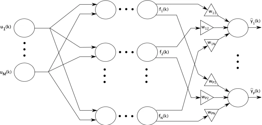
Figure 3.7 General multi-layer neural network topology. . . 39

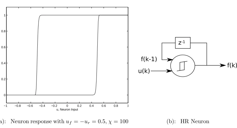
Figure 3.8 HR Neuron structure and representative output . . . 41

Figure 3.9 Topology of Hysteretic Recurrent Neural Network. . . 42

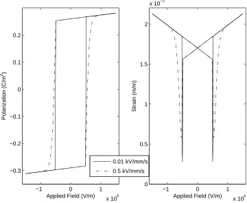
Figure 3.10 HRNN Model: Dependence on rate of applied field . . . 45

Figure 3.11 HRNN Model: Response to applied constant stress . . . 46

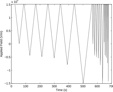
Figure 3.12 Training data: Applied field vs. time . . . 47

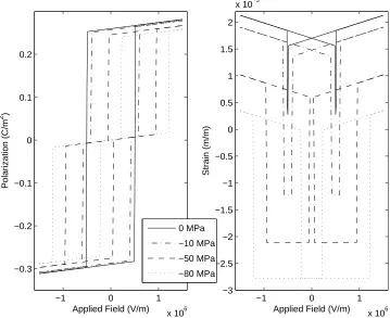
Figure 3.13 Training data: Polarization vs. applied field. . . 48

Figure 3.14 Training data: Strain vs. applied field. . . 49

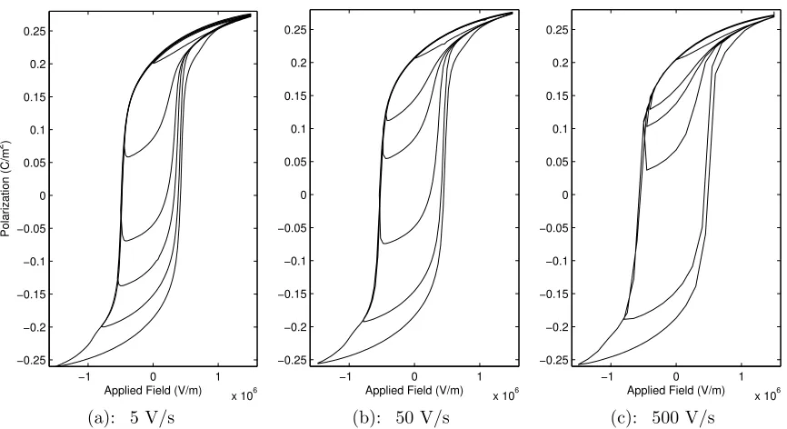
Figure 3.15 Polarization and strain vs. time of best HRNN model (test set, 5 V/s) . . . 52

Figure 3.18 Polarization and strain vs. applied field of best HRNN model (test set, 5 V/s) . . . 55

Figure 3.19 Polarization and strain vs. applied field of best HRNN model (test set, 50 V/s) . . . 56

(14)

Figure 3.21 Log absolute prediction error of RBFN (75 node) and HRNN (α = 100) on test data . . . 59 Figure 3.22 Schematic of actuator coupled to compressive spring. . . 59 Figure 3.23 The Metropolis Algorithm . . . 63 Figure 3.24 Log posterior probability (unnormalized) of chains vs. iteration

number. Vertical line denotes transition from burn-in period to sampling period. Iteration numbers are matched at the end of burn-in. . . 66 Figure 3.25 Samples of PZT physical parameters parameters over final 6000

iterations. . . 67 Figure 3.26 Plot of testing data vs. model output for Bayesian model (Chain 1) 68 Figure 3.27 Testing set cost vs. GA iterations for each run of the optimizer. . 73 Figure 3.28 Actuator polarization (top) and displacement (bottom) vs. time

for slowest loading rate (10 V/s). . . 74 Figure 3.29 Actuator polarization (top) and displacement (bottom) vs. time

for middle loading rate (100 V/s). . . 75 Figure 3.30 Actuator polarization (top) and displacement (bottom) vs. time

for fastest loading rate (1000 V/s). . . 75 Figure 3.31 Normalized distribution of neuron parameters from three

lowest-cost runs. Before training (top), and at lowest-cost minima (bottom). . . 76 Figure 3.32 PI model output vs. time. The top graph shows the results for the

testing set, the bottom shows the performance on the training set, both at 10 V/s. . . 81 Figure 3.33 PI model output vs. time. The top graph shows the results for the

testing set, the bottom shows the performance on the training set, both at 100 V/s. . . 81 Figure 3.34 PI model output vs. time. The top graph shows the results for the

testing set, the bottom shows the performance on the training set, both at 1000 V/s. . . 82 Figure 3.35 Absolute errors in Prandtl-Ishlinskii model and best spring-coupled

HRNN model vs. time. . . 82

Figure 4.1 Schematic of the pintle actuation system in the prototype injector. 85 Figure 4.2 Block diagram of proposed control system. . . 87 Figure 4.3 Schematics of benchtop experiment: (a) mechanical, and (b)

elec-trical. . . 90 Figure 4.4 Experimental setup. (a) The spring sled with PZT stack

(15)

Figure 4.5 RMS model error vs. outer-loop iteration number for 100 and 200-node HRNN models during training. . . 92 Figure 4.6 Output of trained HRNN model with experimental data from

test-ing set (1 Hz). (a) Time response and model error. Lines represent 95% confidence intervals. (b) Comparison of hysteresis loops. . . . 93 Figure 4.7 Output of trained HRNN model with experimental data from

test-ing set (5 Hz). (a) Time response and model error. Lines represent 95% confidence intervals. (b) Comparison of hysteresis loops. . . . 93 Figure 4.8 Data subset from the PAS frequency response experiment showing

two complete periods. The solid line represents the expected re-sponse of a linear system with unity gain and no phase delay. The dashed line represents a cosine fit to the experimental observations (dots). Much of the apparent phase lag is due to the lower slope (displacement/volt) of the PZT actuator in its linear region com-pared to the region where the phase change dominates the strain. One can also observe a broadening of the observed displacement around the trough due to hysteresis. . . 95 Figure 4.9 Response of the open-loop pintle actuation system to step and

si-nusoidal inputs. . . 96 Figure 4.10 Closed-loop response of the benchtop pintle actuation system

sys-tem at four ramp rates, zero-offset case. . . 97 Figure 4.11 Closed-loop responses of the benchtop pintle actuation system at

four ramp rates, 10 mV offset. . . 98 Figure 4.12 Schematic of the injection experiments. Pressure is supplied by the

nitrogen bottle, while the fluid is stored in the fluid reservoir. The solenoid valve controls the fluid flow. . . 101 Figure 4.13 (a) Equivalent circuit model for PZT actuator. Vs represents

ap-plied voltage, Cp represents the capacitance of the PZT element,

and Vp represents voltage due to the polarization of the actuator.

(b) PZT Strain measurement circuit. Voltage measurement (Vm)

is made betweenV1 and V2. Capacitance Cr is chosen to match Cp

as closely as possible. . . 103 Figure 4.14 Actuator displacement measured by the optical sensor (solid line),

and predicted by one- and two-term bridge circuit models. . . 105 Figure 4.15 Closed-loop tracking of pintle displacement reference during 1500psi

spray test, as measured by capacitive bridge circuit. The lower fig-ure displays error and integrated error over time. . . 107 Figure 4.16 Expected and measured spray angles obtained from injection trials

(16)

Figure 4.17 Frames from video of injection trials. Measured boundaries are obtained using automatic edge detection, expected boundaries are

computed based on pintle position. . . 108

Figure A.1 2x Prototype - Injector Body. . . 125

Figure A.2 2x Prototype - Injector Endcap (pintle end). . . 126

Figure A.3 2x Prototype - Injector Endcap (back end). . . 127

Figure A.4 2x Prototype - Mover. . . 128

Figure A.5 2x Prototype - Pintle. . . 129

Figure A.6 1x Prototype - Injector Body. . . 131

Figure A.7 1x Prototype - Nozzle Insert. . . 132

(17)

Chapter 1 Introduction

The preparation of fuel-air mixtures is perhaps the most important topic in combustion

science. The properties of these mixtures determine the energetic and chemical products

of combustion as well as its rate. The evolution of the internal combustion engine has

thus been in lock-step with the evolution of mixing technologies, from carburetors to

throttle-body and port fuel injectors to modern direct injectors. The highly optimized

engines of today rely on fuel-air mixtures prepared to exacting standards.

Improvements in mixture preparation are one way to address a critical problem

presently faced by engine designers: the need to reduce emissions. Regulatory

require-ments (including those of the US Environmental Protection Agency [7]) demand that

diesel engines meet increasingly strict limits on particulate matter (PM, or soot) and

nitrogen oxides (NOx). This is difficult to achieve with conventional diesel combustion

methods which are characterized by a PM-NOxtrade-off (Figure 1.1)[8]. Because

re-actants in conventional diesel combustion are only partially premixed, many reactions

take place in fuel-rich regions. Combustion in such regions gives rise to soot particles

(18)

(promoting soot oxidization), but higher temperatures increase dissociation of diatomic

nitrogen (N2 →2N), resulting in increased NOxformation.

Figure 1.1: Plot of equivalence ratio vs. temperature of combustion, illustrating regions of soot and NOxformation. The curve shows the adiabatic flame temperature of fuel

in air for each equivalence ratio. Regions corresponding to conventional diesel, spark ignition, and HCCI combustion are highlighted. Adapted from [1].

Novel combustion modes such as Homogeneous Charge Compression Ignition (HCCI)

and Premixed Charge Compression Ignition (PCCI) have been proposed to escape this

trade-off by combining a premixed charge (as in spark ignition (SI) engines) with

com-pression ignition (CI), as in conventional diesel engines[9]. The potential benefits of

HCCI are illustrated in Figure 1.1. The question of how to achieve HCCI combustion in

a practical diesel engine, however, remains an open research area. The primary obstacle

to implementing HCCI is the wide range of operation (i.e. idle to full-load) required

by on-road engines[1]. Because HCCI uses a lean mixture to minimize sooting, it is

(19)

As will shortly be shown (Section 1.1.1), dual-mode strategies can be used to overcome

these challenges by using HCCI under partial load and conventional diesel combustion

when full power is required. Because most engine operation takes place at partial loads,

the overall emissions are reduced, but greater power is available when needed (e.g. for

acceleration).

Multi-mode combustion concepts are difficult to implement with conventional fuel

injectors, however, as their fixed spray geometries cannot be optimal for all modes [2].

Thus this dissertation presents the design, modeling, and control of a novel fuel injector

that can provide continuous spray angle control without modulating fuel flow rate or

any other vital injection parameters. The key enabling technologies for this injector are

its externally opening pintle-type nozzle (discussed in Chapter 2), and its actuation and

control systems (discussed in Chapters 3-4).

1.1 Literature Review

1.1.1 Advanced Diesel Combustion

Research on HCCI combustion began in the late 1970s with Onishi et al.[11], who

intro-duced the Active Thermo-Atmosphere Combustion (ATAC) system. The ATAC system

and other early work is summarized in a monograph by Yao et al.[9]. Recently HCCI

research in diesel engines has been driven by a desire to meet increasingly stringent

emis-sions regulations in the US and the EU[7]. Takeda et al. [12] developed a Premixed Diesel

Combustion (PREDIC) system which used early injection from two side-mounted

injec-tors to promote premixed combustion. They demonstrated a reduction in NOxformation

(20)

Combustion (MULDIC) strategy which achieves premixed combustion using an early

in-jection (allowing more time for air and fuel to mix) combined with conventional diesel

combustion from a late injection. Yanagihara et al.[14] and Yanagihara[15] developed the

Uniform Bulky Combustion System (UNIBUS) which uses an early injection to create a

premixed charge, and a later injection to trigger combustion. Yakota et al.[16] tested a

similar system (which they called HiMICS) and found problems with increased

hydro-carbon (HC) and hydro-carbon monoxide (CO) emissions in their experiments. Kook and Bae

[17] also tested a two-stage injection, and found that a narrow (100 ◦) injection angle

of-fered improved performance. Iwabuchi et al.[18] tested premixed combustion using early

injection and reported reduced NOx, but increased HC emissions caused by wetting of

the cylinder liner. To reduce this, they developed a novel injector nozzle with impinging

holes to reduce spray penetration.

In work since 2000, Kimura et al. [19, 20] developed a scheme which used a single, late

injection with high levels of exhaust gas recirculation (EGR) and low compression ratios

to increase charge mixing before ignition. This scheme was called Modulated Kinetics

(MK) and significantly reduced emissions. Gatellier et al.[21] developed a mixed-mode

concept called narrow angle direct injection (NADI), which used HCCI combustion at

low and medium loads and conventional diesel combustion at high loads. The narrow

injection angle allows for early injection without wetting of the cylinder liner. Helmantel

and Denbratt[22] and Lechner et al.[23] also tested early injection with narrow-angle

in-jectors. Kim and Lee[24] tried three different injection strategies with a narrow injector,

achieving significant emissions reductions with a two-stage strategy similar to that of

Yanagihara et al. Su et al.[25] tested pulsed injection, and achieved significant emission

(21)

angle which minimizes wall wetting varies with injection start time (Figure 1.2). A

natu-ral conclusion of this work is that an injector with continuously variable spray geometry

could offer significant flexibility in injection strategies by providing optimal injection

geometry regardless of timing.

(a): 70◦Early (b): 70◦Late

(c): 150◦Early (d): 150◦Late

Figure 1.2: Images of narrow and wide injector sprays from an optical engine. Early images are taken at 52 CAD BTDC, late images at 12.25 CAD BTDC[2].

Fuel injectors with variable geometry sprays have been studied for at least 50 years[27].

In the past 20 years, such designs have focused on enabling advanced combustion modes.

Kato et al.[28] developed an injector in which the spray angle was controlled by the

(22)

Kawaguchi[29] patented a design with an externally opening pintle in which the spray

followed one of two guide surfaces depending on its flow rate. This provided a narrow,

low pressure spray for early injection and a wide, high pressure spray for late injection.

Kawaguchi’s concept was investigated computationally by Ra and Reitz [30] as well as Sun

et al. [31]; simulations showed the potential for significant improvements in emissions.

Hasegawa et al.[32] patented an injector with a rotary actuator in the nozzle that switched

the flow between different groups of holes in the tip. Duffy [33] discussed a mixed-mode

injector developed by Caterpillar which could perform a narrow injection early in the

cycle to promote HCCI combustion combined with a wide-angle late injection to provide

additional power. Busch[34] (of Robert Bosch GmbH) presented an injector with a

so-called Coaxial-Vario-Nozzle which allowed some holes in the nozzle tip to be switched off

at partial engine loads. Jia et al.[35] developed a Micro-Variable Circular Orifice injector,

which modulated the spray’s included angle and droplet size by means of cavitation in

the nozzle region. Sun and Reitz[36] studied a concept in which two injectors were used,

one for a low-pressure early injection and one for a high-pressure late injection. None of

these proposed concepts allow the injection geometry to be controlled continuously and

independently of other injection parameters (e.g. fuel flow rate).

1.1.2 Piezoelectric Materials

The injector discussed in this paper uses a piezoelectric linear actuator to achieve

sub-micrometer position control of a moving pintle at frequencies up to 12,000 rpm (200

Hz) inside the injector nozzle. Thus it is also pertinent to review existing literature on

piezoelectric material physics, modeling, and control problems.

(23)

advantage of their high positioning resolution, such as optics, microscopy, and

micro-electromechanical systems (MEMS). They are increasingly used in electronic fuel

injec-tors because their high bandwidth provides faster needle lift than traditional solenoid

actuators[37], allowing for shorter injection pulses and thus more flexible fuel delivery.

Most research on the modeling of piezoelectric materials can be divided into one of

two approaches. The first approach is based on phenomenological models of hysteresis

such as Preisach operators [38, 39, 40]. These models are often computationally efficient,

but typically their parameters have little or no physical interpretation. The second

group are micromechanical models, which are based on statistical physics. This group

represents material states as a system of coupled, stiff differential equations. One popular

micromechanical model for smart materials is the Homogenized Energy Model (HEM)[6,

41]. Based on the Boltzmann theory of statistical mechanics, the HEM predicts the phase

transition rates of a smart material using an approximate internal energy function. The

predicted transition rates are then integrated in time to determine the material state.

Initial development of this model focused on shape memory alloys [42, 43, 44, 45], but it

has been refined and applied to piezoelectric materials by Smith et al., Ball et al., and

York [46, 47, 6]. An advantage of micromechanical models is that their parameters have

intuitive physical meaning, and many are directly measurable. Solving the differential

equations requires significant computational effort, however, making them poorly suited

to real-time implementation.

Chapter 3 introduces a hybrid model in which the material states are estimated by

a unique neural network, the Hysteretic Recurrent Neural Network (HRNN), but the

remainder of the problem is framed in physical terms. The neurons that make up the

HRNN are specifically designed to capture the underlying hysteresis of single-crystal

(24)

which represents the polycrystalline material.

1.1.3 Control

Real-time control of piezoelectric actuators remains a challenge due to their inherently

non-linear, hysteretic and rate-dependent electromechanical behavior. Classical control

strategies (such as PID) can effectively provide either high bandwidth or high precision,

but typically not both due to these non-linear characteristics[6]. More sophisticated

model-based control strategies seek to address both objectives simultaneously, but require

models that are both accurate and computable in real time. Model-based control systems

for piezoelectric actuators have been extensively studied. Typical approaches include

charge control, inverse model strategies (e.g. feedback linearization or feed-forward model

reference controllers), and feed-forward optimal control.

The charge-control approach involves driving the actuator with a charge-feedback

amplifier (instead of the more usual voltage amplifier). This approach was patented by

Comstock [48], and further developed by Newcomb and Flinn [49], Main et al. [50] and

Kaizuka and Siu [51]. As will be shown in Section 3.4.2, the displacement of a PZT

stack actuator depends only implicitly on voltage, giving rise to hysteresis. Main et

al. develop a formulation in which strain is an explicit function of applied charge, thus

virtually eliminating the hysteresis loops. Their formulation, however, applies only to

unloaded actuators, and has several other drawbacks: Charge-feedback amplifiers are

less widely available than voltage- or current-controlled power supplies, and they require

a sensing capacitor to measure the charge. As discussed in [6], it is difficult to obtain

stable measurements over time due to leakage in the capacitor. Finally, charge-feedback

(25)

non-linearities arising from polycrystallinity.

Inverse model controllers typically involve the choice of a mathematical model for

hysteresis, such as the Preisach [52], generalized Maxwell slip [53], Duhem [54],

Bouc-Wen [55], or Prandtl-Ishlinskii [56] models. Of these models, only the Preisach and

Prandl-Ishlinkii models are discussed in detail here (Sections 3.4.1 and 3.6.4). Typically

such models are easy to train, invertible, and computationally efficient. However, because

they are generalizations, they typically omit important aspects of piezoelectric actuator

behavior such as creep and rate-dependence. These omissions limit the performance of

control systems that make use of them, particularly in operating regimes where these

phenomena are important.

Feed-forward optimal control can be used with any accurate system model, but it is

often employed when techniques such as feedback linearization cannot be used, such as

when the model is not invertible or cannot be computed in real time. Physics-based

mod-els, such as the Homogenized Energy Model of Smith [41], and the

Seelecke-Achenbach-M¨uller model [6], are not suitable for feedback linearization for both of these reasons.

Controllers based on these models instead rely on a priori trajectories; open-loop

opti-mal or sub-optiopti-mal reference inputs are computed off-line. Output feedback is typically

added to compensate for perturbations and unmodeled dynamics. The theory behind

such systems is described in Bryson and Ho [57]. Smith [58] tested a controller based on

these principles for magnetostrictive actuators.

Chapter 4 of this dissertation presents a controller for the VGS injector based on the

HRNN model developed in Chapter 3. This controller uses precomputed feed-forward

(26)

Chapter 2 Injector Design

This chapter discusses the design and testing of a variable geometry spray (VGS) nozzle

for a fuel injector. The design goals were based on the work of Fang in [2]. Assuming

a centrally-positioned injector with a spray angle that targets the piston bowl lip as

the piston advances throughout the compression stroke, the optimal spray angle as a

function of time can be computed from the piston and cylinder geometry. The spray

angle trajectory for a representative piston and cylinder is shown in Figure 2.1. Another

critical design parameter for fuel injectors is the size distribution of droplets in the fuel

spray[59, 60], which depends on the size and geometry of the nozzle outlet, as well as

the pressure and chemical properties (e.g. volatility) of the fuel. This gives rise to

two secondary design objectives for the VGS nozzle: to keep the spray’s Sauter Mean

Diameter (SMD) of spray droplets below 50 microns, and to minimize the variation in

(27)

(a): (b):

Figure 2.1: (a) Spray angle targeting piston bowl lip. (b) Desired injection angle as a function of crank angle.

2.1 Initial Efforts

The author knows of no developed theory that describes the design of a nozzle of this

type. The consensus of the design team was that an externally opening pintle-type nozzle

was the most logical concept to pursue. Such designs produce a hollow cone spray instead

of the solid cone produced by hole-type injectors. The latter are typically used in direct

injection (DI) diesel engines, but the former are common in spark ignition (SI) engines.

A preliminary design based on this concept was produced using solid modeling and rapid

prototyping technology to enable experimental testing as quickly as possible. A cross

section of the initial prototype and the experimental data collected from it are shown in

Figure 2.2. The range of angles produced by this design was not satisfactory, however,

and it forced the design team to re-examine existing design concepts and to move towards

a simulation-based design methodology.

One common household device that produces a hollow-cone spray with a variable

(28)

(a):

1 1.5 2 2.5 3 3.5 4 4.5 5

102 104 106 108 110 112 114 116 118 120 122

Pintle Position (turns)

Spray Angle (deg)

6 psi 10 psi 15 psi

(b):

Figure 2.2: (a) Cross section of the first nozzle prototype, (b) Spray angle vs. pintle position, from low pressure experimental tests with water used as working fluid.

spray nozzles are designed for continuous flow at higher rates and lower pressures than our

fuel injector, the principle of operation is similar to that envisioned for our application. A

garden sprayer was purchased, examined and carefully measured to produce a candidate

nozzle profile (Figure 2.3b). This nozzle section was simulated using commercial

compu-tational fluid dynamics software (CFX, ANSYS, Canonsburg, PA) to determine if such

a simulation could reproduce the range of spray angles observed experimentally. The

results of one such 2D axisymmetric simulation are shown in Figure 2.3c. The success of

these simulations suggested CFD modeling would be a useful tool for simulation-based

(29)

(a): (b): (c):

Figure 2.3: (b) Cross section of the nozzle from a garden sprayer, with pintle insert (c) CFD simulation of sprayer nozzle in intermediate position. Further simulations repro-duced the full range of angles by movement of the pintle.

2.2 Second Prototype

The next design challenge was to rescale the nozzle to a more appropriate size. Because

the size of the annular gap between the pintle and nozzle tip is closely related to the

size of the droplets in the resulting spray, this parameter was used to characterize the

scale. Based on available data for commercial pintle-type nozzles it was determined that

a 100µm annular gap represented a reasonable scale for our second fuel injector

proto-type. There were concerns, however, about the manufacturing tolerances required to

create an injector in which the pintle was centered in the nozzle tip, and whether

avail-able manufacturing services could meet those tolerances. It was determined, therefore,

to perform initial tests on a 2x scale prototype, which could be readily manufactured.

Detailed drawings of the prototype are provided in Appendix A. A nozzle profile with

a 200µm annular gap was simulated using CFX to investigate the relationship between

(30)

The CFD simulations used an Eulerian multiphase model with two phases. Room

temperature air and liquid water were chosen as the reference fluids since those would be

used for the initial experiments. Since CFX simulates 3D geometries exclusively, a single

layer of mesh elements was extruded from a 2D cross section with thickness selected so

as to produce reasonable aspect ratios in the mesh elements. User controls were applied

during the meshing process to ensure a fine mesh in the narrowest regions of the injector.

All simulations solved for steady-state (as opposed to transient) flow, which required the

use of velocity boundary conditions on the inlet. Pressure boundary conditions seemed

to be a more natural choice to replicate experimental conditions but did not produce

convergence using the steady-state solver. Simulations were performed at a variety of inlet

velocities, with low velocities more likely to converge without bootstrapping. For each

pintle position a low-velocity (typically 0.1 m/s) simulation was initialized with an empty

control volume, and run until it converged (as measured by RMS residual magnitudes) to

a steady state. This solution was used as the initial condition for subsequent simulations

with higher inlet velocities. Once each solution reached steady state, the pressure at the

inlet could be computed. This process was repeated until an inlet pressure close to the

target (1000psi) was obtained.

Once the prototype was fabricated, experiments were conducted to confirm the

sim-ulated spray angle/pintle position relationship predicted by the CFD simulations, and

to measure the spray droplet size distribution. These experiments used high-pressure

water (up to 100 bar) as the working fluid, supplied from a small tank pressurized by a

nitrogen bottle. Flow was controlled using an external solenoid valve. A Phantom

high-speed camera (Vision Research, Wayne, NJ) was used to capture images of the spray.

(31)

ap-between those lines (Figure 2.4). A comparison of spray images and corresponding CFD

simulations is presented in Figure 2.5. A plot of observed and simulated spray angles

vs. pintle position is shown in Figure 2.7a. The data support the accuracy of the CFD

simulations in predicting this relationship, and also show that the pressure of the injected

fluid has a negligible impact on the spray angle within the tested range.

(a): (b):

Figure 2.4: (a) Still frame from high-speed video of an injection test, (b) Frame with angle measured.

The size distribution of spray droplets was measured using a Malvern Instruments

(Malvern, Worcestershire, UK) Spraytec laser diffraction instrument. The Spraytec emits

a beam of coherent light which passes through and is scattered by a suspension of

trans-parent droplets in air. The beam is then measured by an array of pickups on the far side.

(32)

Figure 2.5: Still frames from spray videos (left) with corresponding CFD simulation results (right). CFD plots are colored according to flow velocity, lighter colors indicate higher velocity magnitude.

droplets in the sample. Because the hollow-cone spray is likely to scatter the beam

mul-tiple times, the Spraytec also incorporates a proprietary mulmul-tiple-scattering model. The

spray droplets typically have irregular shapes, so some care must be taken in choosing a

measurement to characterize them. The most common metric in combustion science is

the Sauter Mean Diameter (SMD). The Sauter Diameter (SD) is the diameter of a sphere

with the same surface area to volume ratio as the observed particle. Computationally,

(33)

averaging SD over all measured droplets

The results of these tests show a downward trend in droplet size with respect to

pressure, which is promising since the maximum experimental pressure was only 100bar,

one tenth of typical direct injection pressures. The relationship between spray angle and

pintle position is more complicated, and the data are too sparse to make firm inferences.

Figure 2.6 shows both trends as computed from these experiments.

800 900 1000 1100 1200 1300 1400 1500 100

150 200 250

Inlet Pressure (psi)

Sauter Mean Diameter (mm)

0.1mm 0.2mm 0.3mm 0.4mm 0.5mm

(a):

0.1 0.15 0.2 0.25 0.3 0.35 0.4 0.45 0.5 0.55 0.6 100

150 200 250

Relative Pintle Position (mm)

Sauter Mean Diameter (mm)

800psi 1000psi 1200psi 1400psi 1500psi

(b):

(34)

2.3 Third Prototype

In order to reduce the droplet size to more realistic levels and facilitate further

exper-iments, a third prototype with a reduced gap size and pintle diameter was designed.

A 100µm annular gap with a 1.5mm pintle diameter was chosen to be consistent with

commercial scale injectors (a 1x prototype). The reduced orifice area was expected to

produce a spray with smaller droplets. A secondary design goal was conformance with

standard exterior dimensions that would interface with a constant volume combustion

chamber for future experimentation. Thus a “P-type” diesel direct injector was carefully

measured and used to determine the external dimensions of the prototype nozzle.

Over-all dimensions of the injector were significantly reduced to minimize material costs and

produce a more realistically sized device. The previous suite of CFD simulations were

not because the reduced dimensional scale presented numerical problems which led to

inconsistent results.

Spray tests were performed as in Section 2.2, but using isooctane as the working fluid

in place of water. Isooctane (IUPAC name 2,2,4-Trimethylpentane) is a common model

fuel for combustion experiments. The 1x prototype demonstrated an increased range of

spray angles and a decreased pintle stroke. The increased range brings the injector closer

to the desired 160 degree maximum angle, and the reduced stroke makes amplified PZT

actuation more feasible. Plots of spray angle data for the second (2x) and third (1x)

prototypes are shown in Figure 2.7.

The droplet experiments showed a significant reduction in Sauter Mean Diameter, but

the isooctane working fluid prevented the same range of measurements used previously.

For injection pressures above 300 psi the spray absorbed or reflected over 90% of the

(35)

0 0.1 0.2 0.3 0.4 0.5 0.6 0.7 0.8 0.9 1 0 10 20 30 40 50 60 70 80 90 100

Pintle Position (mm)

Spray Angle (deg)

200 psi 500 psi 800 psi 1500 psi CFD (1000 psi)

(a): 2x Prototype

0 0.05 0.1 0.15 0.2 0.25 0.3 0.35 0.4 0.45

0 50 100 150

Spray Angle (deg)

Pintle Position (mm) 500psi

1000psi 1500psi

(b): 1x Prototype

Figure 2.7: Spray angle vs. pintle position, data from CFD simulations and experiments.

size impossible. Measurements were obtained at select pintle positions with a 500 psi

inlet pressure, but at higher pressures too little data was available to draw meaningful

conclusions. From the data available, shown in Figure 2.8, it can be seen that the the

droplet size is below 50µm with 500 psi inlet pressure at most pintle positions (but not the extreme positions that produce the widest or narrowest sprays). One can also infer

that as pressure increases, droplet size decreases for most, if not all, spray angles.

To test electromechanical actuation of this prototype, a piezoelectric (PZT) linear

actuator (PI010.80, Physik Instrumente, Karlsruhe, DE) was used to position the pintle.

As will be discussed in detail in Chapters 3-4, PZT actuators combine high bandwidth

and load capability with sub-millimeter positioning accuracy, making them well-suited to

the requirements of this application. A schematic illustrating the actuator’s integration

with the injector is shown as figure 2.9. Applied voltage causes the actuator to increase

in length; Since it pushes directly on the pintle, this moves the pintle further beyond the

(36)

0 0.05 0.1 0.15 0.2 0.25 0.3 0.35 0.4 30

40 50 60 70 80 90

Relative Pintle Position (mm)

Sauter Mean Diameter (

µ

m)

300psi 500psi

Figure 2.8: (a) Droplet Sauter Mean Diameter vs. pintle position at two inlet pressures, (b) Histogram of droplet diameters at 500psi, 0.4mm pintle position.

spring, which compresses the actuator, causing it to shorten (and thus decreasing the

spray angle) when the applied voltage decreases.

End Cap PZT Stack Actuator Coil Spring

Pintle Pintle Shaft

Figure 2.9: Schematic illustrating direct drive of the pintle by a piezoelectric linear actuator.

High speed video was used to capture the dynamic spray produced by the open-loop

actuated prototype. For these tests an 800V 70Hz square wave input was used to drive

the actuator. Still images from this video are shown in Figure 2.10. The current actuator

(37)

nozzle, but it demonstrates the feasibility of the actuation and control concept. Further

details about the design, as well as closed-loop electromechanical control will be discussed

in Chapter 4.

(a): 0 ms (b): 8.4 ms

Figure 2.10: Frames from video of electromechanically actuated injector driven by a 70Hz square wave input.

2.4 Conclusions

This chapter has described the design and testing of a nozzle for a variable geometry

spray fuel injector. The final (1x scale) prototype produces hollow-cone sprays with

included angles from 20-150 degrees, very close to our design goal of 40-160 degrees. By

aggressively reducing the orifice size, we believe we have achieved our design goal of a

fuel spray with droplets smaller than 50µm SMD, although experimental difficulties make

this somewhat uncertain. Reducing orifice size has also reduced the required actuator

(38)

stack actuator. Although the design will require future improvements (most notably to

incorporate an integral flow control mechanism actuator), the practicality of the VGS

(39)

Chapter 3 Injector Actuation: Design and

Modeling

3.1 Introduction

This chapter discusses the selection of a piezoelectric stack actuator for the VGS injector

prototype, and presents a novel modeling approach that enables high-fidelity real-time

control. The model, based on Hysteretic Recurrent Neural Networks (HRNNs), is unique

in its combination physical principles with real-time performance. Training techniques

for the HRNN based on Gauss-Newton, Bayesian, and genetic algorithms are developed

and compared. Finally, the model is validated against other modeling approaches using

(40)

3.2 Actuator Selection

Electronic fuel injectors have traditionally been actuated electromagnetically using

sol-enoids. Compared to other linear actuators, however, solenoids produce relatively small

forces, with peak blocked stresses of practical devices limited to about 40kPa [61] (limited

primarily by heat dissipation, a particularly acute problem in engines). Fuel pressures for

modern diesel engines typically exceed 1000 bar (100 MPa), so a solenoid cannot oppose

this pressure directly. For this reason modern injectors use the solenoid to operate a

bypass valve, rather than controlling the flow directly (Figure 3.1). Opening and closing

the bypass valve changes the balance of forces exerted by the fuel on the needle or

pin-tle, much like the piloted solenoid valves used in hydraulic or compressed air systems.

This actuation scheme is feasible because most injectors operate in a binary (bang-bang)

mode in which they are either fully opened or fully closed. The proposed VGS injector,

by contrast, requires proportional operation (i.e. positioning anywhere within its range)

with sub-micrometer accuracy. Proportional solenoid valves are used in some

applica-tions, but to the author’s knowledge sub-micrometer positioning accuracy has never been

demonstrated.

Piezoelectric actuators, by contrast, produce relatively large forces (peak blocked

stresses up to 8MPa, [5]) and are commonly used in applications which require high

positioning accuracy, such as atomic force microscopes [62] and micro-electromechanical

systems (MEMS)[63]. The primary limitation of piezoelectric actuators is their relatively

small stroke, limited by a maximum 1% strain [64]. A single layer of piezoelectric

ma-terial (such as the common Lead Zirconate Titanate, or PZT) requires electric fields on

the order of 1kV/mm to achieve its full stroke. Since voltages greater than 1kV are

(41)

Solenoid Fuel Return

Fuel Inlet

Injector Body

Control Chamber _{Injector Needle}

Fuel Reservoir

Bypass Valve

Fuel Spray

Figure 3.1: Schematic of a solenoid-actuated injector. The solenoid is energized, opening the bypass valve and releasing fuel from the control chamber through the fuel return. The resulting pressure drop in the control chamber causes the needle to lift from its seat and fuel to spray into the combustion chamber. Not shown is the return spring which will return the needle once the solenoid is de-energized. (Image by [3], modified by author)

stroke rarely exceeds 10µm, such thin-film actuators are used primarily as micromotors

in MEMS applications.

The stroke of a PZT actuator can be increased by mechanical means, typically using

levers or flexures. These mechanisms exploit classical mechanical advantage to exchange

actuation force for increased stroke. Any simply-supported PZT element can operate as

a flexure, but due to the material’s relatively low tensile strength, it is typically bonded

to a metal substrate when used in this way. One well-known example is the Thin Layer

Unimorph Ferroelectric Driver (THUNDER), Figure 3.2a. Multiple PZT layers may be

bonded to a substrate to multiply the force capacity, resulting in bimorph actuators like

the one illustrated in Figure 3.2b. While such actuators can achieve strokes of up to

1mm, they do so at the cost of greatly reduced forces (often less than 1N) [65, 5], and

are thus also not suitable for the VGS injector.

(42)

(a):

V-PZT

PZT Substrate

V+

(b):

Figure 3.2: A THUNDER unimorph actuator (a), with an illustration of a bimorph actuator (b). (Image from [4])

elements in series to create so-called stack actuators (Figure 3.3). Stack actuators are

composed of layers of piezoelectric material sandwiched between electrodes and bonded

with epoxy. All the elements in the stack are connected physically in series, but

elec-trically in parallel. Because both displacement and required voltage are related to the

thickness of each PZT element, this configuration enables stroke to be increased without

requiring prohibitively large voltages [65]. The principal disadvantage of this arrangement

is that much of the total actuator length is composed of inactive materials (electrodes

and epoxy), so that the strain is typically reduced to about 0.1%.

The most recent VGS injector prototype requires approximately 250 µm of stroke to traverse the desired range of spray angles, which would require a 25 cm stack actuator if

additional stroke amplification were not provided. Although such a long actuator would

be impractical for use in a commercial fuel injector, flexure mechanisms can significantly

increase the stroke of PZT stacks without introducing the excessive friction or backlash

typically associated with levers [66].

Another aspect of piezoelectric actuators that makes them particularly well-suited to

(43)

(a):

PZT Electrode

V-V+

PZT Electrode

(b):

Figure 3.3: Piezoelectric stack actuators with a CD-ROM for scale, (a) and an illustra-tion of stack composiillustra-tion (b). (Image from [5])

of the injector’s pintle position is not feasible in a functioning engine, so the actuator

must self-sense or operate completely open-loop. The development and implementation

of a self-sensing displacement measurement circuit will be presented in Section 4.4.1.

3.3 Physics of Piezoelectricity

The electromechanical behavior of piezoelectric materials arises from their crystal

struc-ture. The presence of unpaired ions (such as T i+4 in P bT iO3) in the crystal lattice

creates a net polarization which causes the lattice to strain in response to an applied

electric field. If the applied voltage exceeds a critical value (the coercive field) the unit

cells of the lattice begin to reorient themselves into a new configuration. This so-called

phase change is the mechanism by which piezoelectrics achieve most of their stroke.

The materials studied here are assumed to have three crystal phases: the 90 degree

(90◦), positive 180 degree (+180◦), and negative 180 degree (−180◦) phases. This is

(44)

[64]. These assumptions follow those in [6], and are generally valid for common

piezo-electric materials, including many formulations of Lead Zirconate Titanate (PZT). The

phase change process is illustrated in Figure 3.4.

An ideal piezoelectric actuator would be composed of a single crystal, in which

each unit cell experienced the same applied stress and electric field, and had the same

phase transition properties. Such an actuator would exhibit strain and

voltage-polarization characteristics similar to those shown in Figures 3.4b and 3.4c (in response

to sawtooth stimulus as in Figure 3.4a) [6]. The remanent strains of the +180◦ and

−180◦ phases would be equal (accounting for the “butterfly” shape of the voltage-strain

curve as in Figure 3.4c), while their remanent polarizations would be equal and opposite.

Within each phase the length of each lattice cell would be a linear function of the applied

field, creating linear changes in strain and polarization. If the critical field value were

exceeded, the lattice cells would transform first to the 90◦ phase, and then (assuming the

starting phase was +180◦) to the −180◦ phase. Unless the material were under stress,

the 90◦ phase would be meta-stable, but always present as an intermediate phase [6].

(a): Applied Field (b): Polarization (c): Strain

(45)

Single crystal actuators are difficult to produce, however, and as a result most

com-mercially available devices are made of polycrystalline materials. Flaws in the lattice

structures of these devices produce internal stresses and distort the applied electric field

in some regions [47]. This has the effect of distributing the coercivities over a range

of values, and producing smooth rather than sharp transitions between phases. This

smoothing can be seen in the experimental data shown in Figures 3.13-3.14.

3.4 Modeling Approaches

The current literature reflects two dominant methods for modeling piezoelectric

materi-als. Most common are phenomenological models built on mathematical representations of

hysteresis (typically Preisach or related Prandtl-Ishlinksii or Kransnosel’skii-Pokrovskii

operators) [68]. These models are built from discrete (or continuous) sets of

individ-ual hysterons (Figures 3.5a and 3.6a). A weighting function is chosen to represent the

distribution of inflection points (where phase changes occur in the material), and the

model output is determined by a weighted sum (or integral) over the hysterons. The

next section presents two of the most significant phenomenological models (the Preisach

and Prandtl-Ishlinskii models) in detail. Other important models include the generalized

Maxwell slip [53], Duhem [54], and Bouc-Wen [55] models.

3.4.1 Preisach and Prandtl-Ishlinskii Models

The Preisach model originated in the study of ferromagnetic hysteresis [69], but has

also been applied to piezoelectric materials [40, 70]. The development here follows that

(46)

The model is generalized to polycrystalline materials by a weight function µ(α, β). The model output is computed by integrating the product of the kernel and weight function,

f(t) =

Z Z

(α,β)∈S

µ(α, β)γα,β(u(t)) dβdα, (3.1)

where u(t) is the input, and S is a set in the Preisach plane (Figure 3.5b) which includes all past inputs, S = {(α, β) : umin ≤ β ≤ α, umin ≤ α ≤ umax}. It is usually

required thatβ ≤α, so only the upper half of the plane is used. This infinite-dimensional model is capable of representing arbitrarily complex hysteresis loops, but in practice

finite-dimensional approximations are implemented instead [71]. The classical Preisach

model is inherently rate-independent, and even its discrete version represents the material

state by storing an arbitrary number of past input extrema (theoretically requiring infinite

memory). Several ways of implementing rate-dependence within this framework have

been explored, including [72, 73, 74, 75, 76].

+1

-1

u_r u_f

γ_u f,ur

u

(a):

α β

u_max umin

S

u_min umax

(b):

Figure 3.5: (a) The output of a Preisach hysteron (γα,β) with transition points α and

(47)

The Preisach model has evolved over time, giving rise to a family of models more

read-ily applied to practical devices. The Prandtl-Ishlinskii (PI) model is one such derivative,

which has the advantage of being analytically invertible [71]. The PI model replaces

the Preisach relay operator with a composition of two operators, the play (or backlash)

operatorH, which captures the hysteresis, and the superposition operatorS, which mod-els the memory-free non-linearities in the system. The characteristic functions of these

operators are shown in Figure 3.6. The play operator can be defined recursively by

y(ti) =Hrh(x(ti), y(ti−1))

y(t0) =Hrh(x(t0), zh0) (3.2)

Hrh(x, y) = max{x−rh,min{x+rh,0}}

where y is the output, x is the input, rh is the transition threshold, and zH0 is the

initial state of the operator. The superposition operator is written

y(ti) =Srs(x(ti)) (3.3)

Srs =



    

    

max{x−rs,0} rs >0

x rs = 0

min{x−rs,0} rs <0

where rs is the threshold.

(48)

Hr

-r_h

r_h y

x

(a):

Sr

r_s y

x

(b):

Figure 3.6: (a) Play operatorHr(u) characteristic, with transition points r and −r and

input u. (b) Superposition operator Srs(u), with transition pointrs.

threshold-discrete PI model

P(t) =wT_s ·Srs w

T

h ·Hrh(x(t), ZH0)

, (3.4)

where ws and wh are weight vectors for their respective operators. The thresholds

also become vectors, with rh ={rh,0 < rh,1 <· · ·< rh,nh},

rs = {rs,−` <· · ·< rs,−1 < rs,0 < rs,1 <· · ·< rs,`}, and ns = 2`+ 1. A more detailed

derivation of the model can be found in [71].

The PI model described to this point is rate-independent, as is the classical Preisach

model. Kuhnen [76] developed a scheme for incorporating rate-dependence into the PI

model by means of a creep operator

y(ti) =Krk,ak(x(ti), y(ti−1)) (3.5)

which is defined as the solution to the differential equation

d

(49)

where ak is an eigenvalue analogous to the time constant of linear ODEs. [76] does

not specify how this equation is to be solved, but for the purposes of this dissertation a

forward Euler scheme was used.

The creep operator is incorporated into the model as an additive hysteresis,

P∗(t) = w_sT ·Srs w

T

h ·H(x(t), Zh0) +wkT ·Krk,ak(x(t), zk0)·i

, (3.7)

where i = (1,1,· · · ,1) is a column vector of ones. Both rk and ak become vectors

with multiplicity nh and nm, respectively. TheK operator becomes an nh x nm matrix

of allrk,i,ak,i pairs

Krk,ak(x, zk0) =

        

Krk,0,ak,1(x, zk001) · · · Krk,0,ak,nm(x, zk00nm)

Krk,0,ak,1(x, zk001) · · · Krk,1,ak,nm(x, zk01nm)

..

. . .. ...

Kr_k,nh,ak,1(x, zk0nh1) · · · Kr_k,nh,aknm(x, zknhnm)

         . (3.8)

One key advantage of this model is that it is fully invertible, enabling straightforward

analytic design of feed-forward controllers. It is also, like the HRNN, uniquely determined

by its current and previous inputs. This is a significant advantage over the classical

Preisach model, which requires potentially unlimited storage of past extrema.

3.4.2 Internal Energy

Another popular approach is to model the internal energy landscape of the material.

Assuming that the phase state minimizes the actuator’s internal energy, one can use

(50)

approach was explored by Seelecke, Achenbach, and M¨uller for shape memory alloys

[42, 43, 44, 45] , and has been applied to piezoelectric materials by Smith et al., Ball

et al., and York [6, 47, 41], among others. The internal energy is modeled by a set

of piecewise-continuous polynomial functions of strain, polarization and applied electric

field. The probability of transitioning between phases is determined by the magnitude

of the potential barriers between the minima of these functions. The evolution of the

material phases over time is computed by solving ordinary differential equations which

depend on the transition probabilities. Because the transition probabilities change

radi-cally in the neighborhood of certain critical points, these ODEs are inherently stiff. Since

they are solved in the time domain, this method has the advantage of exhibiting rate

de-pendence as a natural consequence of thermal activation. However, extending the model

to polycrystalline actuators is not trivial. Existing implementations are computationally

intensive, making them difficult to apply in real-time settings such as servo control.

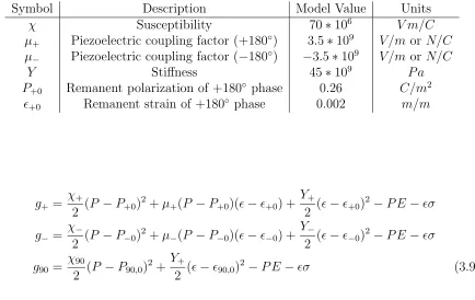
Details of a particular free energy model will be summarized here; this formulation

is detailed in York [6]. The Gibbs energy densities g of the actuator are taken to be quadratic functions of polarization (P), strain (), applied electric field (E), and stress

(σ) as well as the material properties given in Table 3.1. Energy densities for each phase

are presented together as Equation 3.9. This approach represents a simplification of

the Landau-Devonshire expansion, which uses higher-order polynomials. The quadratic

(51)

Table 3.1: Symbols and representative values for PZT material properties. Values given are those assumed in the HRNN model. Where no phase is specified, the property is assumed to be the same for all phases.

Symbol Description Model Value Units

χ Susceptibility 70∗106 _{V m/C}

µ+ Piezoelectric coupling factor (+180◦) 3.5∗109 V /m or N/C

µ− Piezoelectric coupling factor (−180◦) −3.5∗109 _{V /m} _or _N/C

Y Stiffness 45∗109 _{P a}

P+0 Remanent polarization of +180◦ phase 0.26 C/m2

+0 Remanent strain of +180◦ phase 0.002 m/m

g+=

χ+

2 (P −P+0)

2

+µ+(P −P+0)(−+0) +

Y+

2 (−+0)

2₋

P E−σ g−= χ−

2 (P −P−0)

2₊_µ−(P ₋_P−

0)(−−0) +

Y−

2 (−−0)

2₋_{P E}₋_σ

g90=

χ90

2 (P −P90,0)

2₊ Y+

2 (−90,0)

2₋_{P E}₋_σ _(3.9)

The probability pαβ of the material transitioning between two phases α and β is

modeled by the Boltzmann distribution, resulting in Equation 3.10. The transition

prob-ability is a function of the Gibbs energy as well as the material relaxation time τx,

Boltzmann’s constant kb, absolute temperature T, and lattice element volume Vle, as

well as the polarization and strain values at the barrier separating α fromβ, denoted Pb

and b respectively.

pαβ =

1 τx

e−g(E,σ,Pb,b)Vle/kbT

RPR

e−g(E,σ,P,)Vle/kbT d ∂P

(3.10)

Obtaining a solution to Equation 3.10 is not tractable in most cases. In the limit of

(52)

3.11 (as shown in [6]). Equation 3.11 is formulated in terms of the magnitude of the

energy barrier between the states, ∆gαβ. Calculation of this energy barrier is also not

trivial, and the reader is again referred to [6] for a detailed discussion.

pαβ =

1 τx

e−∆gαβVle/kbT _(3.11)

The evolution of the material’s phase fractions in time can be written as a system of

differential and algebraic equations depending on the phase fractions xα, and transition

probabilities. This system is Equation 3.12 for the simplified case in which transitions

from the +180◦ to−180◦ phase are not allowed. This assumption is based on the work

of Li and Fang[77]. p90+ refers to the probability of transitioning from the 90◦ to +180◦

phases, while p+90 refers to the reverse.

˙

x+=x90p90+−x+p+90

˙

x−=x90p90−−x−p−90 (3.12)

x90= 1−x+−x−

Once the phase fractions are known, the macroscale properties of the material can

be written as linear combinations of the average properties of each phase. In Equations

3.13 and 3.14, polarization and strain are written in terms of the expected values hPαi

(53)

P =hP+ix++hP−ix−+hP90ix90 (3.13)

=h+ix++h−ix−+h90ix90 (3.14)

Assuming low thermal activation as above, the desired average properties are equal to

the values at the Gibbs energy minima [6]. The following equations can thus be obtained

by minimizing Equation 3.9 with respect to polarization and strain.

hP+i=

Y+E+µ+σ

χ+Y+−µ2+

+P+0 h+i=

χ+σ+µ+E

χ+Y+−µ2+

++0

hP−i= Y−E+µ−σ χ−Y−−µ2

−

+P−0 h−i=

χ−σ+µ−E χ−Y−−µ2

−

+−0 (3.15)

hP90i=

E χ90

+P90 h90i=

σ χ90

+90

3.5 Hysteretic Recurrent Neural Networks

For the VGS injector project, a model was sought that combined the best elements of the

Preisach and internal energy approaches: namely the physical parameterization of the

Seelecke model and the computability of Preisach approaches. This dissertation proposes

a solution based on the Hysteretic Recurrent Neural Network developed by Veeramani

et al.[78]. The HRNN is used to capture the hysteretic phase change characteristics

of piezoelectric materials (replacing the ODE of Equation 3.12). The remainder of the

model is based on constitutive equations for strain and polarization described in section

Design, Modeling, and Control of a Variable Geometry Spray Fuel Injector.

ABSTRACT

DEDICATION

BIOGRAPHY

ACKNOWLEDGEMENTS

TABLE OF CONTENTS

LIST OF TABLES

LIST OF FIGURES

Chapter 1

Introduction

1.1

Literature Review

1.1.1

Advanced Diesel Combustion

1.1.2

Piezoelectric Materials

1.1.3

Control

Chapter 2

Injector Design

2.1

Initial Efforts

2.2

Second Prototype

2.3

Third Prototype

2.4

Conclusions

Chapter 3

Injector Actuation: Design and

Modeling

3.1

Introduction

3.2

Actuator Selection

3.3

Physics of Piezoelectricity

3.4

Modeling Approaches

3.4.1

Preisach and Prandtl-Ishlinskii Models

3.4.2

Internal Energy

3.5

Hysteretic Recurrent Neural Networks