Scholarship at UWindsor
Scholarship at UWindsor
Electronic Theses and Dissertations Theses, Dissertations, and Major Papers
2016
An Efficient FPGA Implementation of Optical Character
An Efficient FPGA Implementation of Optical Character
Recognition System for License Plate Recognition
Recognition System for License Plate Recognition
Yuan Jing
University of Windsor
Follow this and additional works at: https://scholar.uwindsor.ca/etd
Recommended Citation Recommended Citation
Jing, Yuan, "An Efficient FPGA Implementation of Optical Character Recognition System for License Plate Recognition" (2016). Electronic Theses and Dissertations. 5832.
https://scholar.uwindsor.ca/etd/5832
This online database contains the full-text of PhD dissertations and Masters’ theses of University of Windsor students from 1954 forward. These documents are made available for personal study and research purposes only, in accordance with the Canadian Copyright Act and the Creative Commons license—CC BY-NC-ND (Attribution, Non-Commercial, No Derivative Works). Under this license, works must always be attributed to the copyright holder (original author), cannot be used for any commercial purposes, and may not be altered. Any other use would require the permission of the copyright holder. Students may inquire about withdrawing their dissertation and/or thesis from this database. For additional inquiries, please contact the repository administrator via email
Optical Character Recognition System for
License Plate Recognition
by
Yuan Jing
A Thesis
Submitted to the Faculty of Graduate Studies through the
Department of Electrical and Computer Engineering in Partial Fulfillment
of the Requirements for the Degree of Master of Applied Science at the
University of Windsor
Windsor, Ontario, Canada c
by
Yuan Jing
APPROVED BY:
Dr. Rupp Carriveau
Civil and Environmental Engineering
Dr. Roberto Muscedere Electrical and Computer Engineering
Dr. Mitra Mirhassani, Advisor Electrical and Computer Engineering
I hereby certify that I am the sole author of this thesis and that no part of this thesis
has been published or submitted for publication.
I certify that, to the best of my knowledge, my thesis does not infringe upon
anyones copyright nor violate any proprietary rights and that any ideas, techniques,
quotations, or any other material from the work of other people included in my
thesis, published or otherwise, are fully acknowledged in accordance with the standard
referencing practices. Furthermore, to the extent that I have included copyrighted
material that surpasses the bounds of fair dealing within the meaning of the Canada
Copyright Act, I certify that I have obtained a written permission from the copyright
owner(s) to include such material(s) in my thesis and have included copies of such
copyright clearances to my appendix.
I declare that this is a true copy of my thesis, including any final revisions, as
approved by my thesis committee and the Graduate Studies office, and that this thesis
Optical Character Recognition system (OCR) has been found very useful in the field
of intelligent transportation. In this work, a FPGA-based OCR system aimed at
image-based License Plate Recognition (LPR) has been designed and tested. A
feed-forward neural networks has been chosen as the core of the proposed OCR system.
The neural network parameters are acquired beforehand and will not change during
its operation time. A set of Matlab programs have been made in the network’s design
process. The verification process includes Matlab simulation where programs using
binary numbers which has the same representation format as the system to compute
the results, and Modelsim simulation where data is computed and transferred between
modules under clock signals’ control. The synthesis process is done in the Altera’s
FPGA design software - Quartus II. The result shows that calculation speed of the
system implemented in hardware is much faster than software running on a PC while
it maintains a high recognition accuracy. The proposed image recognition system is
used with a set of images that are generally difficult for such networks to handle.
Most images include shadows and other imperfections in the image. The proposed
network was able to achieve 95% accuracy in recognizing the correct character despite
While I was working on this thesis I received numerous help from many people and I
would like to take this chance to express my thankfulness. I received valuable advices
and help from my fellow lab members Babak, Iman, Bahar and Rose and they are
very good persons to work with. I also want to thank members of my committee Dr.
Rupp Carriveau and Dr. Roberto Muscedere for their valuable time and feedbacks.
Last but not least, I want to extend my sincere appreciation to my supervisor Dr.
Declaration of Originality iii
Abstract iv
Dedication vi
Acknowledgments vii
List of Figures xii
List of Tables xiv
List of Symbols xv
Glossary xvi 1 Introduction 1 1.1 Problem Statement . . . 2
1.1.1 Challenges . . . 2
1.1.2 Dataset . . . 3
1.1.3 Objectives . . . 4
1.2 General System Configuration . . . 4
1.4 Overview of Character Segmentation System . . . 7
1.5 Overview of Optical Character Recognition System . . . 8
1.6 Thesis Organization . . . 10
2 Feedforward Neural Network 11 2.1 Introduction of Artificial Neural Networks . . . 12
2.1.1 History of Artificial Neural Network . . . 12
2.2 General Theory of Feedforward Neural Network . . . 14
2.2.1 Forward Propagation Phase . . . 14
2.2.2 Training Phase . . . 16
2.3 System Description . . . 17
2.4 Determining the Size of the Neural Network . . . 17
2.4.1 Three Layers Versus Four Layers . . . 18
2.4.2 Number of Inputs to the First Layer . . . 19
2.4.3 Number of Nodes in the Second Layer . . . 21
2.5 Network’s Training and Testing . . . 22
2.5.1 Recognition Accuracy of the Network . . . 24
2.6 Summary . . . 27
3 Network Implementation 28 3.1 Arithmetic Format . . . 29
3.1.1 Binary Fixed-Point Format . . . 29
3.1.2 Binary Floating-Point Format . . . 30
3.1.3 Comparison Between the Two Representation Formats . . . . 32
3.2 Activation Function . . . 33
3.2.1 Approximation Method . . . 34
3.2.2 Errors of Approximation Method . . . 36
3.2.4 Processing Region . . . 41
3.3 Determining the Size of the Fixed-Point Numbers . . . 43
3.4 Summary . . . 48
4 Network’s Implementation in Hardware 49 4.1 System Description . . . 50
4.1.1 Parallelism . . . 50
4.1.2 FPGA . . . 53
4.1.3 Network Parameters . . . 54
4.2 Data Path . . . 55
4.2.1 First and Second Layer . . . 55
4.2.2 Third Layer . . . 59
4.3 Control Path . . . 60
4.3.1 Clock Signals . . . 61
4.3.2 Other Control Signals . . . 63
4.4 Summary . . . 64
5 RTL Simulations 66 5.1 Network Synthesis . . . 66
5.2 RTL Simulations . . . 67
5.3 Comparison with Other Works . . . 69
5.4 Summary . . . 71
6 Conclusion 73 6.1 Contributions . . . 73
6.2 Suggestions for Future Work . . . 75
References 76
1.1 Frequency of characters in the dataset . . . 3
1.2 General block diagram of a License Plate Recognition system . . . . 5
2.1 Generic structure of a 3-layer feedforward network . . . 14
2.2 Computation model of an neuron in an artificial neural network . . . 15
2.3 Characters in different resolutions . . . 21
2.4 Recognition accuracies of networks with different sizes . . . 22
2.5 Samples of characters in the dataset . . . 23
2.6 Examples of misclassified characters . . . 26
3.1 Positive range of an 1-2 floating-point number . . . 31
3.2 Different regions defined in hyperbolic tangent function . . . 35
3.3 Quantization error and estimation error in this activation function ap-proximation method . . . 37
3.4 Regions determined by different None . . . 38
3.5 Error in pass region . . . 39
3.6 Activation function in saturation region . . . 40
3.7 Computations in ANN in binary . . . 44
4.1 Waveform of inputs and output of a memory block . . . 56
4.3 Waveform of inputs and output of an adder tree . . . 57
4.4 Block diagram of the feedforward network . . . 62
4.5 Loading second layer’s parameters . . . 62
4.6 Clock and control signals of comparator . . . 65
5.1 Synthesis results of feedforward network . . . 67
5.2 A block diagram of this feedforward network . . . 68
1.1 Comparison of different classification methods in OCR . . . 9
2.1 Recognition accuracies of 3-layer and 4-layer feedforward neural networks 19 2.2 Input size of several feedforward neural networks used for LPR appli-cation . . . 20
2.3 Recognition accuracies from different groups of training data . . . 26
3.1 All positive values represented by 1-2-1 floating point numbers . . . . 31
3.2 Number of bits of FXP and FLP for different requirement . . . 33
3.3 Comparison of errors caused by fixed-point number representation . . 46
3.4 Errors caused by fixed-point format in hidden layer and output layer 47 4.1 Comparison of SOP parallelism and MAC parallelism . . . 52
5.1 Comparison of software simulation and hardware simulation . . . 69
5.2 Comparison of different hardware-implemented networks . . . 70
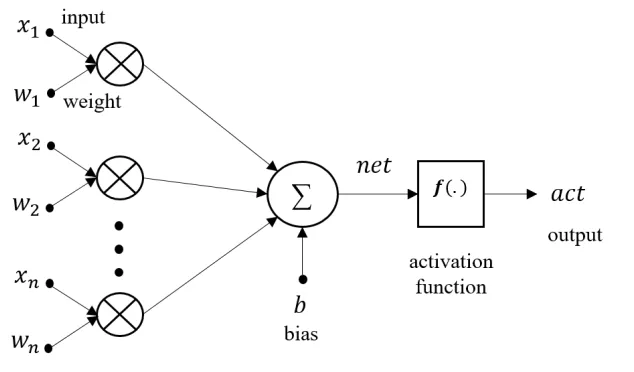
netji : The summation of the multiplications of inputs and corresponding weights of
ith neuron in jth layer.
actji : The output of ith neuron in jthlayer.
wjki : the weight between ith neuron to the kth output in the previous layer.
bji : The bias of ith neurons in jth layer.
numE : The number of exponential bits.
numM : The number of mantissa bits.
tanh : Hyperbolic tangent function.
ea : Approximation error.
eq : Quantization error.
None : The place of first non-zero bits in a binary number(except the sign bit).
xpaq : The boundary between pass region and processing region.
xsq : The boundary between processing region and saturation region.
Ni : The number of integer bits.
Nf : The number of fractional bits.
OCR : Optical Character Recognition
FPGA : Field Programmable Gate Array
LPR : License Plate Recognition
LPD : License Plate Detection
CS : Character Segmentation
CCA : Connected Component Analysis
SVM : Support Vector Machine
HMM : Hidden Markov Model
ANN : Artificial Neural Network
CPU : Central Processing Unit
FXP : Fixed-Point
FLP : Floating-Point
LUT : Look-Up Table
PWL : Piece-Wise Linear
MSB : Most Significant Bit
LSB : Least Significant Bit
MAC : Multiply-ACcumulate
LE : Logic Element
PLL : Phase-Locked Loop
RAM : Random Access Memory
MUX : Multiplexer
Introduction
Automatic License Plate Recognition has been applied in applications such as
auto-matic toll collection, traffic control and monitoring, as well as parking lot control and
access [6, 26, 16]. These systems are becoming more important as the automotive
industry moves toward autonomous driving and smart roads. In these applications,
the system should be able to find and recognize the characters on the plate and be
operational in a variable environment. The road and weather condition, as well as
lighting, creates numerous challenges for these systems. Although the task is very
easy for humans, a fully automated system with full recognition, in the presence of
1.1
Problem Statement
1.1.1
Challenges
The input characters that are fed to an LPR are not as complicated as those in other
applications such as handwriting or facial recognition application. However, the input
image still creates challenges for the recognition processing [31].
Due to its application, the location of a plate is not at the same place between
different images. The cars’ relative location to the camera can differ. Therefore the
camera has to look for a plate in all areas of a picture. Moreover, an image might
contain one or multiple plates. Each of these plates has to be processed and recognized
by the system.
Other issues include changes in font, color and background images on a plate. For
example, plates can be different in color and font, and may contain a logo, symbols
and other features that generally are not present in regular plates. Even standard
plates differ between various provinces as well as countries.
In addition to these, dirt or obstructive material on the plate can cause the system
to fail to detect and recognize the characters. Environmental issues such as image
background prevent most systems to be adopted for in an ad hoc manner. Each
system has to be installed, trained, and tested which in turn increases the total cost
and complexity of the scheme.
Another important variation that can cause problems is the quality of the license
plates. License plates in poor conditions can make the input characters very noisy.
Therefore, the capability of recognizing noisy or deformed input can be another
ele-ment in causing the system to fail or make mistakes.
Most systems cannot resolve all of the features with cognitive computing resources.
Moreover, most of the works reported in the literature are based lab test, and image
Figure 1.1: Frequency of characters in the dataset
that the system is not limited and focuses on using images that have various font
colors, and illumination and lighting are non-uniform. In the next section, general
LPR system and its sub-blocks are introduced.
1.1.2
Dataset
The images of license plates used in this work are taken in Ontario, Canada. The
latest version of Ontario’s license plates uses the font of ’Driver Gothic’. The dataset
contains many images of segmented characters. These images are acquired from
386 images taken at parking lots at different locations. The images of characters
are segmented from the images containing whole license plates. Each license plates
contains six to eight characters. The letter ’I’ and the number ’1’ will be considered
as the same character. Moreover, the letter ’O’ and the number ’0’ are the same. The
frequency of appearance of alphabetical characters in the dataset is shown in Fig.
1.1. It is a common fact that not all the characters are used in LPR systems [33]. In
general, most license plates avoid using both of these characters on the same plate.
The system in this work will keep all the four outputs, as these characters can look
recognition accuracy is calculated, it will be considered as a correct recognition for
both ’0’ and ’O’.
1.1.3
Objectives
The system designed in this thesis is the decision-making system of an Optical
Char-acter Recognition system for License Plate Recognition applications. The inputs to
the system are images of characters resized to the same size uniformly. The system
is supposed to be able to determine the input character.
The aim of this work is to implement an FPGA-based feedforward neural network
which is suitable for a particular classification problem. The FPGA gives a popular
platform for this implementation task. The flexibility of designs in FPGA makes
the network capable of dealing with similar problems with minor modification of
conception. More importantly, the hardware-based neural network tends to have
a faster processing speed with similar or fewer hardware resources compared with
PC-based neural networks implementations. In software-based ANNs like PC-based
neural networks, neurons are modeled by programs running on general-purpose CPUs.
However, the PC-based model is running on the processors that executing instructions
sequentially, which essentially in contradiction with the parallelism of neural networks.
FPGA is chosen as the platform for the implementation of ANN for this work. The
basic processing units in FPGAs give them the parallel data processing ability.
1.2
General System Configuration
Figure 1.2 is a general block diagram of a typical License Plate Recognition (LPR)
system.
The images can be taken by a color, black, and white, or an infrared camera. Most
Figure 1.2: General block diagram of a License Plate Recognition system
using a very high-resolution camera is discouraged in most applications.
The task of the License Plate Detection (LPD) system is to determine if the input
image contains the image of a license plate and to find its location on that picture. At
this stage, the unnecessary parts of the image are discarded, and the system focuses
on the essential component of the image that contains the plate(s). An optimal
system should be able to detect the presence of a license plate in an image from all
the background information, as well as overcome the challenges in the image.
Next gate is the Character Segmentation (CS) system, which takes the image of
a plate and separates the characters from each other. At this stage, elements such
as dirt, shadow, angled image, and vanity plate backgrounds can cause issues for
the system. The outcome of the CS system is only to separate the characters from
each other. Recognizing them is the job of the next block which is the focus of this
research.
The Optical Character Recognition (OCR) is an integral part of LPR system.
Efficient hardware implementation of the OCR is the center of this study, and will
be explained in detail in later chapters. In the rest of this section, a brief overview
units were not implemented in this research, and results from simulations were used
in order to feed the hardware implementation of the OCR system.
1.3
Overview of License Plate Detection System
There are a number of works available in the literature that deal with various aspects
of a License Plate Detection. In order to implement an LPD, different types of
features are used to detect the license plate area from the background. Some of the
most common features used in these works include color, shape and texture [27, 4, 31].
In [27] color is used as the feature to detect license plates, while [4] used the
geometric character of the license plates to detect them. However, These methods
are not very reliable since the desired background color of a license plate or the
rectangular shape of the license plate can be absent because of the complex conditions
in the real environment.
In comparison, methods that rely on features such as the texture of the license
plates are more reliable [31]. Vertical gradient has been found to be a very efficient
method to select license plate areas. The license plate area when compared with the
background, is a vertical edge intensive area due to the present of characters. Methods
using vertical edges [31] usually convert the images into a gray-scale image, then the
vertical gradient is computed for the whole picture. A filter is then applied to the
result to select the area with the highest vertical edges. The threshold for selecting
the highest range can be adaptive, and the result may contain several candidates. By
setting a threshold or aspect ratio of the size of license plates, the non-license plate
1.4
Overview of Character Segmentation System
When the presence of a license plate is detected in an image, the characters on the
plate has to be separated from each. The Character Segmentation System has to
acquire the full image of a license plate and to deliver a set of separated characters
to the next block. Different methods are proposed in literature for implementation
of the CS system [25, 7, 13].
Vertical and horizontal projection [25, 7] are common methods in Character
Seg-mentation. Because of the gap between each character on the plate, the vertical
projection of the license plate image will observe a low-value region and characters
can be separated. However, this method can not process images with tilted license
plates. Since the relative position between a license plate and the camera can vary,
all characters in a picture will not always appear on a horizontal line. Therefore the
gap between the adjacent characters is no longer vertical.
This problem can be solved by a rotation correction done by the Hough transform
[13]. However, this method is computationally intensive.
The Connected component analysis(CCA) is a useful method for segmentation
method. The CCA analyses the image, and all adjacent pixels holding certain value
or above will be considered as one component. By applying the CCA to the image
of the license plate, each character will be seen as a part. All characters will be
acquired by filtering all of the elements through a threshold value such as the size of
1.5
Overview of Optical Character Recognition
Sys-tem
Both the detection and segmentation systems act before the OCR are the necessary
pre-processing steps. This thesis focuses on the hardware design and implementation
of the OCR portion of the scheme.
Many different classification methods have been proposed for the OCR
applica-tions [11, 5, 19]. Classification is a process to that separates the observaapplica-tions into
different, predefined categories based on the features of the observations [11]. This is
a restricted definition of general classification but is similar to the supervised learning
in machine learning field.
The classification rules in statistics are called statistical models. From the concept
that whether or not there are a clearly defined statistical models, classifiers can be
categorized into statistical classification methods and machine learning classification
methods [5].
Statistical classification methods tend to look at the classification problem as a
statistic process. The other methods tend to emphasize on the performance of the
OCR system other than understanding the underlying mathematical model.
Com-mon statistical classification methods used in OCR include support vector machines
(SVM)[19], hidden Markov models (HMM), and template matching. On the other
hand, artificial neural networks(ANN) can be seen as machine learning classifiers.
Table 1.1 provides a high-level comparison between several OCR systems. There is
no significant difference in the recognition success rate between the various methods.
However, due to the different conditions that testing data are acquired and different
size of the testing dataset, a simple comparison between table values is not sufficient.
More analysis and tests are required to verify the success rate of a certain method
References Character Recognition Method Recognition Accuracy Processing Time
[29] HMM 95.2% 0.1s
[10] HMM 95.7% Not reported
[28] HMM 97.5% 0.1s
[14] Template Matching 95.7% Not reported
[17] Template Matching 97.3% * 0.9s
[30] SVM 97.2% less than 1s
[8] ANN 97.7% not reported
Table 1.1: Comparison of different classification methods in OCR
* The OCR recognition accuracy is not provided by the author. The value used here is estimated
based on the overall success rate and the success rate in character segmentation step.
Another issue that needs to be considered is the complexity and computation
re-quirements of different methods. It is critical to have an algorithm with less
computa-tional complexity for hardware implementations of the OCR system. The algorithms
used for the OCR usually contain two parts; feature extraction and classification
[31, 5, 35]. The extra step for performing the feature extraction requires more
arith-metic operations which mean more adders and registers in hardware. The success
of the SVM methods and HMM methods is heavily based on a good selection of
extracted features. On the other hand, ANN and template matching methods can
process the raw data from the character segmentation steps.
Template matching methods calculate the Euclidian distance or Hamming
dis-tance between pixels in testing input and templates. The ANN method can use all
of the pixel values from the input images directly as its inputs. Apart from
compli-cated arithmetic operations that template matching method requires, it also needs a
significant number of temples in different conditions in order to be able to recognize
characters in all different conditions correctly. Taking all these factors into
of it was developed.
1.6
Thesis Organization
The thesis is organized as follows. Chapter two discussed the feedforward neural
networks - the OCR method in this work. An introduction of feedforward neural
network as well as the procedure of determining the structure and size of the
feedfor-ward neural networks in this work are given. In chapter three, issues in implementing
the network in hardware are discussed. This includes the arithmetic format used in
this system, implementation of the activation function and the bit width of the
num-bers in this system. Chapter four implements the system on a FPGA. The parallel
scheme as well as the design of data path and control path of the system are given
in this chapter. The system is a synchronized system. Using different clock signals
in different blocks is a critical design process for realizing parallelism and pipelining
in the system. RTL simulations are given in chapter five. The performance of this
system is compared with other hardware and software OCR systems. In chapter six,
Feedforward Neural Network
Feedforward neural network belongs to a class of artificial neural networks. In order
to implement the OCR section a feedforward Neural Network is used. This type of
network is inspired by the biologic neural network even though they are very different
in terms of their essential characteristics.
The basic unit in an ANN is a neuron, whose name came from the cells in a
nerve system. An artificial model of a neuron in an ANN is more computationally
complex than its biological counterpart. In this chapter, the theory of the feedforward
neural networks and characteristics of artificial neurons are reviewed. Design criteria,
limitations, and used process for the proposed network are provided. These are used
to set the network size and the required number of neurons in each layer. Simulation
results of the network during the training and recognition stages using Matlab are
2.1
Introduction of Artificial Neural Networks
Like machine learning, ANNs’ ultimate goal is to bring intelligence to machines [11].
That is to let machines have consciousness instead of merely giving a response to
the stimuli. Artificial Intelligence has many achievements and is applied in many
applications in different areas such as image recognition and speech recognition[21].
However, there is still a long way to go before machines can act, make decisions, or
think like a human.
Despite the astonishing computing power and the high computation accuracy,
computers lack some of the critical abilities such as adaptability due to experience.
The ANN is provided by this feature and has been used in applications that require
interaction with humans such as advertising. The main difference between the ANNs
and a conventional computer is that an ANN is composed of massively parallel yet
simple computing units [23].
2.1.1
History of Artificial Neural Network
In 1949 Donald Hebb proposed a theory in his book [15] of how the neuron works based
on his observation. The idea is that the more stimulation, the stronger connection
between these two neurons. Based on this he proposed the Hebbian learning rule.
The first practical implementation of ANN is the perceptron which was invented in
late 1950’s by Frank Rosenblatt. The perceptron networks are good at classification
problems. However, the classes must be linearly separable. This problem is well
recognized after Marvin Minsky, and Seymour Papert pointed it out in their book
[22] published in 1969.
After that, the research of ANN started to cool down. For a long time, many
researchers tried to find a way to overcome this challenge. In the late 1960’s when
implementation of multilayer feedforward neural networks became possible[3]. This
method started to draw attentions by its reintroduction by Paul J. Werbos, Geoffrey
E. Hinton, and Ronald J. Williams in 1980’s [24].
The back-propagation learning algorithm enables the network architectures to
have multi-layered structures. Hence these are far stronger than the perceptron
net-works. The multi-layered networks can theoretically model any non-linear functions
in any degree of complexity. The back-propagation training algorithm is a
signifi-cant step forward for the research of ANN and made the implementation of network
structures possible. Nowadays, the deep learning techniques make feedforward neural
networks more powerful in solving many problems. The training process will be done
in anther platform, which makes it an off-line version of ANN. The reason for this is
that for the same application, there is no need to train the network once the network
is properly trained. Also, the training phase compared with the recall phase is much
more computationally intensive, requires a lot of memory. FPGA may not be capable
of doing the training process since the gradient calculations involved in the training
process. Some researchers have proposed new learning algorithms which are
differ-ent from the gradidiffer-ent calculation based method, and suitable for the FPGA platform.
However, finding a suitable ANN solution for the real life complex problem sometimes
need the trial and error technique, and many different architectures are required to
be tested in the companion of the corresponding training procedures. Feedforward
neural networks are data-driven applications of supervised training. Training data is
crucial to the training phase, and how good the training phase is done determines
how well the network will perform. In this chapter, the theory of a feedforward neural
network, including the structure of its core units - neurons and the training process is
discussed. The dataset which consists of training data and testing data are described
Figure 2.1: Generic structure of a 3-layer feedforward network
2.2
General Theory of Feedforward Neural
Net-work
The general structure of a feedforward neural network is showed in Figure 2.1. Each
circle in the figure represents a neuron. A feedforward neural network consists of
many neurons; these neurons form the layers in neuron network. There is no data
transfer between neurons in the same layer; neurons only send data to neurons in
the next layer. Feedforward neural network is a widely used type of neural network
structure because of its relatively simple structure and effectiveness in classification
problems.
2.2.1
Forward Propagation Phase
The outputs of the feedforward neural network can be acquired by calculating the
outputs of all neurons layer by layer. This process of calculating the outputs of
a neural network is the forward propagation phase. Since the neuron is the basic
Figure 2.2: Computation model of an neuron in an artificial neural network
neuron.
Figure 2.2 shows the structure of a neuron. Each neuron in a multilayer
feedfor-ward neural network computes a weighted sum of its inputs. These inputs are outputs
of all the neurons from the previous layer. The neuron’s output is the weighted sum
regulated by an activation function. The computation of each neuron’s output can
be expressed as
actji =f(netji) (2.1)
where f is the activation function, and actji is the output of the activation function
of the ith neuron in the jth layer, and netji is the summation of the multiplications
of inputs and corresponding weights of ith neuron in jth layer.
The value of the netji can be obtained as follows:
netji =
m
X
k=1
actjk−1wkij +bji (2.2)
wheremis the number of neurons in the (j−1)th layer,bj
i is the bias ofith neurons in
jth layer, and wj
ki is the weight between this neuron to thek
layer.
2.2.2
Training Phase
Most neural networks and in particular feedforward networks can not be used before
the networks have been properly trained. Feedforward neural networks are trained by
the supervised learning algorithms, where input-target pairs will be utilized during
the training phase. A cost function is used to indicate how well the training is done.
The cost function used in training phase is a mean square error function:
E =
1
2
n
X
i=1
(acti−ti)2 (2.3)
wheren is the number of neurons in the output layer,acti andti are the actual output
and ideal output of the network respectively.
This cost function represents the difference between the ideal and actual outputs.
The training of the neural network is a process of adjusting neural network parameters
in such a way that the real output is closer to ideal output. The study shows that the
feedforward neural networks will get the best performance by minimizing this cost
function.
E(wnew) = E(w+ ∆w) (2.4)
Using the Taylor series, an estimation of this equation can be obtained:
E(w+ ∆w) = E(w) + ∂E
∂w∆w (2.5)
To minimize E we need to minimize ∂E
∂w∆w. ∂E
∂w is the gradient which is an
n-dimensional vector pointing to the directions which make the function E increases
the most. Due to the fact that the dot product of two vectors will result in a smaller
value if both vectors pointed to the opposite directions while they have the same
length, the above equation can be modified as follows:
∆w=−α∂E
where α is a coefficient that controls the steps of learning.
The training technique for feedforward neural networks is called backpropagation,
which calculates the partial derivatives using the chain rule.
2.3
System Description
The training phase will be done in the design process, and the system in hardware
will only perform the forward propagation phase. The value of network parameters
will be calculated in software and sent to the memories in the hardware system.
In designing the feedforward neural network, Matlab has been used as the design
software. Its powerful computation ability and versatile design approaches make it
very suitable for the task. Also, the neural network toolbox integrated into Matlab
makes the training of the networks much faster and the design time will be greatly
shortened. The network design process in Matlab will be two parts, first is to use
Matlab design a feedforward neural network, during this process all the network
parameters will be determined, this includes the size of the network and the size and
format of the input data. The second step is to verify the simulation results using
Matlab. However, the codes are specially designed so that all the operations are done
in binary format to simulate the computations in FPGA.
2.4
Determining the Size of the Neural Network
The number of nodes in the second layer is used to increase the network accuracy.
However, a larger number of nodes in the network requires more data for it’s
super-vised learning phase. No equation can provide the correct size of a neural network.
Therefore in this section, simulations are used to create an early estimate of the
network size, using Matlab simulations. Using the images in the dataset a Matlab
efficient size for the network.
2.4.1
Three Layers Versus Four Layers
It has been claimed in [18] that a three-layer feedforward neuron network with at
least one hidden layer is able to model any systems with any degree of complexity.
However, feedforward neural networks with more than 3 layers can also be used in
classification applications. In this section, structures of feedforward neural networks
with 3 layers and 4 layers will be compared in terms of performance and computation
intensity.
The optimized structure of a 3-layer feedforward neural network for this
applica-tion whose determining process is described in this chapter has a structure of
189-160-36. These numbers are the numbers of nodes in the input layer, 2nd layer and
output layer, respectively. A feedforward neural network with 4 layers is used to
compare with. The two networks will have the same number of hidden neurons and
to make the design simple, the two hidden layers of the 4-layer feedforward neural
network will have equal number of neurons. Therefore, the structure of the 4-layer
feedforward neural network is 189-80-80-36.
Because of that the inputs are 1-bit binary numbers, the real multiplications
be-tween input signals and their corresponding weights of the neurons in a layer happens
in the third layer and the fourth layer. The number of multiplications needs to be
done in a complete recognition process for one character is 160×36 for the 3-layer
network and 80/times80 + 80/times36. That is a 61.11% more multiplications need
to be performed for the 4-layer network.
On the other hand, the performance of the network is another concern. Table
2.1 listed the recognition accuracies of feedforward neural networks with different
structures. The first three rows are the networks with 4 layers and the last row is the
Network structure Recognition accuracy
189-60-60-36 95.16%
189-70-70-36 96.15%
189-80-80-36 96.34%
189-160-36 96.81%
Table 2.1: Recognition accuracies of 3-layer and 4-layer feedforward neural networks
performance get better. However, even though the network with the same number
of hidden neurons has a performance which is less than its 3-layered counterpart.
Considering the reasons discussed above, the proposed system in this thesis will have
a three-layered structure.
2.4.2
Number of Inputs to the First Layer
Trained by a supervised learning algorithm, the feedforward neural network is a
data-driven classifier. Its performance is highly related to the format of input data.
More-over, the features used for this application are all the pixels from the re-sized, and
segmented images. Therefore the size of the network, or more specifically, the size of
the input layer of the network depends on the size of input vectors if every image is
treated as a vector.
The used camera in this work was set around 2 to 3 meters away from the license
plate when the images were taken. The input of the neural network depends on the
resolution of character images for a fixed size network. Therefore, all of the character
images were resized to a uniform value. The expected size of a character is 56×23,
with the aspect ratio(height divided by width) equal to 2.368. These values were
derived from the average resolution images. The sample size is 10% of the dataset.
However, the number of the nodes in the first layer will be equal to the resolution
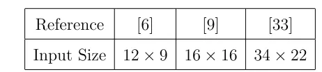
Reference [6] [9] [33]
Input Size 12×9 16×16 34×22
Table 2.2: Input size of several feedforward neural networks used for LPR application
this resolution is quite large, and it will inevitably lead to a larger size for the neural
network. The size of the network is a critical aspect which needs to be considered
especially for hardware implementation.
Table 2.2 listed the sizes of input layer of feedforward network in some LPR
systems. Clearly 56×23 is a resolution larger than any of these. Such big resolution
will lead to a big network whose memory and multiplier requirements can be hardly
supported by a single FPGA chip with high parallelism in its computation process.
Therefore, a resize process for the raw character images was necessary and a smaller
resolution for the input characters needs to be determined.
A much smaller resolution can still be able to represent all the English letters and
Arabic numbers. However, smaller resolutions require higher image quality in order
to be recognized correctly. In other words, smaller resolutions are more sensitive to
noises and deformed images. Images with relatively more complex strokes such as
’H’, ’M’ and ’W’ are easily become impossible to be recognized in small resolutions
with some noises. So the desired size of input image should be less than 56×23 at
the same time not too small to recognize character images with noise. So the rules
to choose a smaller size of input images are first, keep the same aspect ratio to keep
the characters the same as the original images as possible. The aspect ratio found in
10% of the samples of the data set is 2.34. Among the resolutions fall in the range
of resolutions similar to those listed in Table 2.2, 14×6, 21×9, 28×12 and 35×15
have the closest aspect ratios to 2.34. The last resolution will lead to an extensive
network which is hard to be implemented in a single FPGA. Therefore, only the first
Figure 2.3: Characters in different resolutions
rule is to leave enough space between vertical strokes. Figure 2.3 list characters in
these resolutions. Characters on the left and middle and right have the resolutions of
14×6, 21×9 and 28×12, respectively. It can be seen that some characters in the
resolution of 14×6 lost the details that are crucial to the correct recognition while
the other characters generally keep the details.
Therefore, the second resolution which is 21×9 is chosen, and all input characters
will be resized to this resolution, and input layer has a size of 189.
2.4.3
Number of Nodes in the Second Layer
An experiment was done to test the performance of the networks with different sizes
in order to determine the network’s optimal size. In this experiment, the character
images in 96 out of 386 license plate images were used as the testing input. The
remaining 290 license plate images were used as the training data.
In this setup, the number of nodes in the second layer was set the variable
com-ponent. The experiment tested the performance of networks with a various umber of
nodes in the second layer. The range of the number of nodes for the second layer was
limited from 100 to 200 with a step of 20. This range is broad enough to cover the
For each condition, the network was trained, and its performance was calculated
10 times. The average value was used for comparison purposes. Figure 2.4 shows the
recognition accuracy of different network settings.
In Figure 2.4 the horizontal axis is the number of nodes in the second layer. It
can be seen that the recognition accuracy increases with the number of neurons in
the second layer, and it reaches its highest point where the number of neurons is
160. From this result 160 is the most suitable number of nodes for the network’s
second layer. There must be some errors as only 10 samples are used to estimate the
expectation of the population. However, the trend will be the same.
Figure 2.4: Recognition accuracies of networks with different sizes
2.5
Network’s Training and Testing
In this section, the network’s performance will be evaluated after the network is
trained. The date used for training is necessary for the network’s performance. Some
Figure 2.5: Samples of characters in the dataset
The difficulty in recognition task comes from two elements; one is that some
characters have very similar shape. The second element is the distortion. These two
problems can be alleviated to some degree by training the network with more data.
Thus, a training set with enough training data is essential for a successful training.
For an ANN, the number of required training data is related to the number of
parameters it has. A significant input layer has more parameters to train, and that
requires a larger dataset of training data. Moreover, as it can be seen from Figure 1.1,
the frequencies of letters appeared in all images are far less than those of numbers.
Although some letters are not prohibited in license plates, but they only appear in
some special cases. For example, ’G’ and ’U’ only appeared less than 5 times in
all samples. Therefore, there is no chance for the feedforward neural network to be
able to recognize these characters successfully with such a small size of the training
2.5.1
Recognition Accuracy of the Network
When the optimum size for the feedforward network was determined, the network
was trained and tested with the dataset. This feedforward neural network is a
three-layered network with 189 inputs, 36 outputs and 160 neurons in a hidden layer.
The first layer or input layer’s neurons only send input data to the hidden layer.
The neurons in the second layer or the hidden layer compute the functional value
of the weighted sum of input data. The neurons in the third layer or output layer
compute the final output of the network.
Usually, the activation functions for a neural network are the same in neurons
in the same layer. Functions that are typically used as activation functions include
logistic function, linear function, and hyperbolic function. Experiments show that for
this classification problem, hyperbolic functions are the best choice for both neurons
in the hidden layer and output layer. In this thesis neurons in hidden layer and output
layers use the hyperbolic tangent function as the activation function.
The dataset including images created from ideal character images was divided
into training data and testing data. The test data was only used to verify network’s
performance after the training is finished. In other words, the network has not seen
the testing data during the training phase.
To choose the images for the training data, 10% of images were randomly selected
and marked as the validation images. During each iteration, validation images were
processed by the network. However, these results were not used to guide the network
and were only used to compare network’s performance through iterations.
If the error kept growing for a certain number of iterations, then the training was
stopped to prevent the problem of over-fitting. This technique is particularly useful
when the size of training data is small compared with the number of parameters that
the network has. In here the maximum value 6 was used.
process were reused in network verification process. In order to keep the verification
result as convincing as possible, a n-fold cross-validation was used for testing network’s
performance.
Considering the size of the available dataset, a n = 4 is used here. A total of
386 images was divided into four groups, each containing 96, 96, 96, and 98 images
respectively. Each group was used as testing data and the network’s performance
over all groups was averaged. During each cluster as testing data, the rest data in
the dataset was used as training data. In this way, the network can be tested using
all samples in the dataset.
The learning algorithm used in this case is scaled conjugate gradient, which is a
technique to solve optimization problems. This algorithm is suitable for optimization
problems with a large amount of parameters such as the feedforward neural network
in this thesis.
Every time network’s parameters are initialized with different values, and the
net-work’s recognition accuracy varies from time to time. As the starting point changes
every time, it will settle down at the various minimum point at the surface. The
highest recognition accuracy for different initializations can not represent this
net-work’s recognition accuracy because the network can’t see the testing data during
the training phase. Once the training phase is done, the network’s parameter will not
change while it is processing the data.
Data created from the method described in the previous section will be used as a
supplement to the testing data from the dataset. In order to show the effectiveness of
the supplementary training data, a comparison of recognition accuracy of a network
which is trained by different training datasets, will be presented.
Table 2.3 shows the results of the recognition accuracy of a network trained with
various training data. The numbers in the second row are the accuracy rate of testing
Testing Data Group1 Group2 Group3 Group4 Average
recall accuracy 0.9927 0.9960 0.9942 0.9938 0.9942
recognition accuracy 0.9833 0.9681 0.9653 0.9856 0.9756
Table 2.3: Recognition accuracies from different groups of training data
Figure 2.6: Examples of misclassified characters
accuracy of the network for different testing data. It can be seen that this value gets
better for the group 1 and group 4 more than the others. This is because that most
of the failed recognitions are caused by distorted character images, and the images in
adverse conditions are not uniformly distributed across the whole dataset.
Figure 2.6 shows the misclassified characters from a testing of data in group 3.
A value of 97.56% is the expected recognition accuracy achieved by the network
2.6
Summary
In this chapter an introduction of feedforward neural network is given. A
simulation-based design methodology is provided for designing a feedforward neural network
for this application. The simulation results shows the potential performance of the
hardware version of this network design. The parameters of the network acquired from
simulations using data from group 1 as testing data will be used in the designing of
the network in hardware. In the rest of this thesis, the requirement of recognition
accuracy for the designed network is to reach the same level as the results of Matlab
Network Implementation
As the structure and parameters of the network has been decided, the next task is to
implement the network on an FPGA platform. For a hardware implementation of the
network, more effort is required to maintain the same level of accuracy in comparison
with the simulations due to the limitations of resources in the hardware devices. One
major issue related to the accuracy is the limited number of bits that can be used to
represent the Sigmoid activation function. Rough estimates of the activation function
will prevent the network from getting trained properly.
Therefore, the goal in this hardware implementation was to control and keep
the error of the activation function within a reasonable range. The process for this
3.1
Arithmetic Format
From a computational perspective, a neuron is a nonlinear function of its inputs.
Multiplication, addition, and a non-linear activation function are the essential
com-putational operations of a neuron.
The format of the number representation has a significant influence on the
com-putational precision and the final area that is required for implementing the network.
This is a common trade-off between the cost and the performance. Therefore, an
appropriate numerical precision should be chosen that can satisfy the error
require-ments while it does not use too much hardware resources.
Here, the two most commonly used binary number representation formats in
dig-ital circuits are considered; fixed-point, and the floating-point representations. These
two representation formats will be examined in terms of precision for numbers with
same or similar ranges as well as their areas requirements for implementation of adders
and multipliers.
3.1.1
Binary Fixed-Point Format
A fixed-point binary number can be represented by
SImIm−1...I2I1I0.F−1F−2...F−n+1F−n (3.1)
whereS is the sign bit,I is the integer part, F is the fractional part, and i∈[−n, m].
Each S, I, and F, represent a single bit binary number. Together, they form a
fixed-point value.
The radix point sits between the integer and fractional parts. The sign-magnitude
value for this representation is calculated as follows
V = (−1)S×(Σmi=0Ii×2i+ Σ−1i=−nFi×2i) (3.2)
For the sign-magnitude, fixed-point binary representations, the range of values
The range of this representation is mainly controlled by the number of the integer
bits. If the fractional bits’ contribution to the representation range is ignored, then
it will be doubled every time the number of integer bits increases by one.
The precision of this representation is controlled by the number of the fractional
bits. All of the values that can be represented by this format are evenly distributed
across the range at 2−n intervals. By increasing the number of fractional bits, the
precision increases.
3.1.2
Binary Floating-Point Format
Floating-point numbers consist of one sign bit, mantissa bits, and exponential bits.
SMmMm−1...M2M1M0.E−1E−2...E−n+1E−n (3.3)
The value of a binary floating point number is calculated as follows:
V = (−1)S ×1.M ×2E−bias (3.4)
where
E = Σni=1E−i×2n−i (3.5)
and
bias= 2numE−1−1 (3.6)
Where numE is the number of bits for the exponential parts, numM is defined as
the number of the mantissa bits.
The representable range of values for floating point numbers depends on the
num-ber of exponential bits. AsnumEincreases, the range increases exponentially.
There-fore, one advantage of binary floating-point format over fixed-point format is the larger
representation range.
Figure 3.1 is an example of the positive part of a 1-2-1 floating-point number.
Figure 3.1: Positive range of an 1-2 floating-point number
E M1 M0 value
0 0 0 1
0 0 1 1.25
0 1 0 1.5
0 1 1 1.75
1 0 0 2
1 0 1 2.5
1 1 0 3
1 1 1 3.5
Table 3.1: All positive values represented by 1-2-1 floating point numbers
be derived from the equation 3.6 that 2numE−1 −1 = 0 when numE = 1. In order
to get a clearer view of this representation, all the possible positive values of it are
listed in Table 3.1.
The precision of the representation depends on both the number of exponential
bits and mantissa bits. To better illustrate the impact that numE and numM have
on the precision, two terms are defined here. Alargeintervalmeans a range of values
that can be represented by the same exponential bits. A basicinterval means the
interval between two adjacent values that can be represented by this number format.
The value of the numE determines the number of large intervals (in this case the
into basic intervals.
The value of the numM determines the number of basic intervals that large
in-terval includes and it is the same for all large inin-tervals. However, the range of large
intervals grows as number increases. This, in turn, causes the basic intervals to grows
as well. Therefore the precision of binary floating-point representations is dynamic
in its range. The closer to the origin the more precise the number will be.
3.1.3
Comparison Between the Two Representation Formats
In this section, the performance of the two representation formats is compared. This
early stage comparison allows the designer to make a more informed decision.
The values of integer bits, fractional bits, mantissa bits and exponential bits are
represented asnumI,numF,numM andnumE respectively. The range that a
Fixed-Point (FXP) or an Floating-Floating (FLP) number can express is determined by
numI for the FXP and numE for the FLP. Both numF and numM ascertain the
accuracy of the FXP numbers and FLP numbers respectively.
The previous analysis showed that the advantages of floating-point representation
over fixed-point are that it can cover a larger range ifnumI andnumE are the same.
However, this larger range is acquired at the cost of low accuracy for larger numbers.
This is pointed out by Figure 3.1, where the number of basic intervals is the same
for all regions divided by the different value of E. As the range of region increases,
the accuracy of this number representation drops.
Table 3.2 illustrates the number of bits to acquire certain range and number
representation accuracy for both FXP numbers and FLP.
From the table, it can be seen that for the task of representing numbers in a
certain range while keeping the same representation accuracy over the whole range,
FLP requires more bits than the FXP.
range accuracy FXP FLP
24−1
2−4 4-4 3-7
2−5 4-5 3-8
2−6 4-6 3-9
25−1
2−4 5-4 4-8
2−5 5-5 4-9
2−6 5-6 4-10
26−1
2−4 6-4 4-9
2−5 6-5 4-10
2−6 6-6 4-11
Table 3.2: Number of bits of FXP and FLP for different requirement
the implementation of the adder in floating-point representation requires as much as
ten times of hardware as it in fixed-point representation implementation [32] shows.
However, the multiplier implementation in floating-point requires about half of
hard-ware resources of it in fixed-point implementation [32] shows. Considering the
dif-ference of hardware requirement for implementation as well as the number of adders
will be much more than the number of multipliers, it is better to use fixed-point
representation than using floating-point representation for this implementation of the
feedforward neural network.
3.2
Activation Function
The fixed-point number format is chosen as the arithmetic format used in this work.
Therefore, the next step is to implement the Sigmoid activation function in the
The general definition of the Hyperbolic tangent function can be expressed as
tanh(x) = e
x−e−x
ex+e−x (3.7)
This function can not be directly implemented in hardware efficiently because of the
division and exponential computations. Therefore, different approximation methods
have been proposed for implementing this function in hardware.
3.2.1
Approximation Method
Look-up table method [12] samples hyperbolic function at constant intervals and
stores the values into memories. The output of the look-up table is the stored
func-tion value. In order to keep the approximafunc-tion error in a small range, a certain
number of samples are needed. The more samples stored in the memories, the more
precise the functions will be. Therefore, the size of the look-up table (LUT) function
approximation method will be a concern.
Piece-wise linear (PWL) [1] approximation has a different strategy. The nonlinear
function is replaced with many linear functions in various parts in its domain. The
curve of the hyperbolic tangent function is divided into many areas. Straight lines are
used to approximate the curve in each of these small regions. The approximated value
of the input to this function is calculated based on the function of the corresponding
line. Instead of storing all the values at different points, the PWL method [1] requires
to implement several linear functions, and the approximation error is closely related
to the number of piece-wised linear functions.
The procedure in [34] has been used in this work to implement the activation
func-tion. This method is similar to an LUT method. However, the memory requirement
is small for same approximation criterion. This method implements the activation
function using fewer circuits while the error is guaranteed to be less than a certain
Figure 3.2: Different regions defined in hyperbolic tangent function
of the hyperbolic tangent function. The main idea is to divide the whole domain into
three regions. Here the analysis will only consider the positive numbers since the
hyperbolic tangent function is symmetric with respect to the origin.
Pass region covers the range that close to the origin. Since Equation 3.7 is
differ-entiable in its domain and f0(x) = 1−f2(x), the approximation value around x= 0
by using first order Taylor series can be expressed as
f(x) = f(0) +f0(0)(x−0) (3.8)
From Equation 3.7, f(0) = 0, and f0(0) = 1, the function can be approximated as
f(x) = x (3.9)
when x is close to 0.
When the input exceeds a certain value, it enters saturation region. In this region,
region is properly set, the output can be expressed as a constant
f(x) =C (3.10)
while keeping the error within an accepted range.
The processing region is the region between the pass region and saturation regions.
In this region, the derivative of the function with respect to the input decreases when
the input increases. This means that the function tends to change at a slower speed
with increasing input. Therefore, if a binary number is used to represent a range of
the function, then the range is not the same over all of the processing region. This
method is called range-addressable look-up table.
3.2.2
Errors of Approximation Method
The total error in this approximation consists of quantization error, eq, and
approxi-mation error ea. The quantization error is caused by the binary format of the input
number, and ea is caused by approximation method as well as the binary
represen-tation of output number. This can be seen clearly in Figure 3.3 : The curve stands
for the target function which needs to be approximated, and the step function is an
approximation of it. The three consecutive inputs are displayed as x1, x2 and x3
re-spectively. When the value of an input such asxfalls into the region ofx2, the output
for this input will be fa(x2). The quantization error eq in this case is |f(x2)−f(x)|,
and the approximation error is|fa(x2)−f(x2)|. Therefore the total error is as follows:
e=eq+ea
=|(f(x2)−f(x)) + (fa(x2)−f(x2))|
(3.11)
where f(x2)−f(x) and fa(x2)−f(x2) may have different signs and the two errors
sometimes may partly canceled by each other.
So this situation illustrated in Figure 3.3 is a worse case where they have same
Figure 3.3: Quantization error and estimation error in this activation function
ap-proximation method
For inputs in pass region which are close to the origin, the difference between the
hyperbolic function and f(x) = x approximation can be omitted. This means that
ea is almost zero and error comes from eq.
As the input moves towards positive infinity, ea increases. In saturation region,
since the output is a constant, there is no eq and only ea is left. In the processing
region, both eq and ea need to be considered.
The boundary between the pass and processing regions and between the
process-ing and saturation regions, as well as the number of fractional bits for both input and
output, have to be decided carefully to make certain activation function’s
Figure 3.4: Regions determined by different None
3.2.3
Determining the Boundaries Between the Regions
In this section, the two boundaries, xpaq and xsq, which divided the whole domain
into three regions will be determined.
The input value determines which region and which subranges in the processing
region the output is placed.
One way to make comparisons between two binary numbers is to compare them
bit by bit from most significant bit(MSB). Therefore, a variable None is defined to
indicates the place of the first non-zero bit (except the sign bit) in a binary number
in the form of sign-magnitude. The None has the same value as the weight of this bit
when the value of a binary number is calculated using equation 3.2.
For example, a binary number 0110.0111 has a None = 2 and 0000.1111 has a
None =−1. The place of the first non-zero bit, or None, determines the possible value
of this number. This can be seen more clearly in the Figure 3.4. Every time None
increases by 1, the range of the number it can represent is doubled.
First, the boundary between the pass and processing regions xpaq is going to be
determined.
Figure 3.5 shows the error of the activation function represented by f(x) = x
in the pass region. The top figure shows three functions. The curved line is the
Figure 3.5: Error in pass region
function is f(x) = x implemented in binary. This example uses a step of 0.1 for the
reason of demonstration. In the implementation the step size is equal to 2−n where
n is the number of fractional bits.
The lower figure shows the difference between the step function and hyperbolic
tangent function. When the input is close to the origin, the straight line and
hyper-bolic tangent function are almost the same. However, the error represented as the
comb-like shape in the bottom figure is still unacceptable.
This is the quantization error which is caused by the binary representation and it
has a maximum value of 2−Nf. The value of the N
f has to be large enough to make
sure 2−Nf ≤.
As the input increases, the error has a trend of increasing. The quantization error
is still the same. If the is set to a certain value such as 0.1 in this example (the
Figure 3.6: Activation function in saturation region
The first boundary xpaq is determined by fstep −tanh(x) = , that is when the
total error is greater than the maximum allowable error. However, when this function
is computed, the step function, fstep, is replaced with f(x) = x. This is because if
epsilonis set as 2−Nf, then the error will not be greater thanbefore the step function
and hyperbolic tangent function separate.
After these two functions separate, the error only increases every time whenf(x) =
x and the step function share the same value. Therefore, if is set to be equal to
0.04, by solving this functionxpaq = 0.5098.
The next step is to calculate the boundary between the processing and saturation
regions, xsq. Figure 3.6 shows the hyperbolic function. The maximum value the
function’s binary representation can have is Ymax = 1−2−Nf.
Moreover, as the input increases, the hyperbolic function approaches 1. Therefore,
the value of the error in the saturation region is equal to 1−(1−2−Nf) = 2−Nf. In order
to keep the error less than , the requirement for Nf is the same as the requirement
from pass region. The boundaryxsqcan be determined from 1−2−Nf−tanh(xsq) =,