Doubly-robust Estimators in Observational Studies with and without a Stratified Sub-sample.

(1)

ABSTRACT

BAI, XIAOFEI. Doubly-robust Estimators in Observational Studies with and without a Stratified Sub-sample. (Under the direction of Anastasios A. Tsiatis.)

In this dissertation, we study semiparametric estimators in observational survival analysis. Observational studies are frequently conducted to compare the effects of two treatments on

survival. For such studies we must be concerned about confounding; that is, there are covariates

that affect both the treatment assignment and the survival distribution. With confounding the usual treatment-specific Kaplan-Meier estimator might be a biased estimator of the underlying

treatment-specific survival distribution and the ordinary log rank test might lead to biased

result.

This dissertation has three parts. In Chapter 1, we use semiparametric theory to derive

doubly robust estimators (and their asymptotic variance) of the treatment-specific survival

distributions and the difference in the treatment-specific survival distributions in the case when the collected covariates are enough to adjust for all confounding in the main study. In Chapter

2, we develop treatment-specific survival estimator in the case when we further conduct a

stratified sampling substudy to collect additional potential confounding covariates. In Chapter 3, we develop log rank type test statistics to test for the difference in overall treatment curves,

in both case of main study and substudy. All developed methods are applied to a real data

(2)

(3)

Doubly-robust Estimators in Observational Studies with and without a Stratified Sub-sample

by Xiaofei Bai

A dissertation submitted to the Graduate Faculty of North Carolina State University

in partial fulfillment of the requirements for the Degree of

Doctor of Philosophy

Statistics

Raleigh, North Carolina

2014

APPROVED BY:

Marie Davidian Daowen Zhang

Wenbin Lu Anastasios A. Tsiatis

(4)

DEDICATION

(5)

BIOGRAPHY

The author was born in Beijing, China. She entered Nankai University and obtained the Bach-elor’s degree in Statistics from the College of Mathematical Sciences in 2009. She began her

graduate study in the statistics department at North Carolina State University and got the Master’s degree in 2011 on the path of pursuing a Ph.D. degree. With the valuable instruction

and guidance from her adviser Dr. Anastasios (Butch) Tsiatis, she focused working on

(6)

ACKNOWLEDGEMENTS

I would like to take this opportunity to express my sincere gratitude and appreciation to my adviser, Dr. Anastasios (Butch) Tsiatis, who provided me insightful instruction and generous

support throughout my research and my dissertation. He has always been encouraging and understanding and showed great patience and kindness to me. I learned a lot from Dr. Tsiatis,

not only on the expertise knowledge in statistics but also on how to conduct research work. I

feel very lucky to have him as my adviser. Without his help and guidance, I would not be able to accomplish this work.

I am greatly grateful to my committee members, Dr. Marie Davidian, Dr. Daowen Zhang

and Dr. Wenbin Lu, for reviewing my dissertation and sharing their insightful comments and suggestions to my research. I would like extend my appreciation to all the faculty members of the

Department of Statistics at North Carolina State University, who offered a variety of interesting

and useful lectures. I also want to thank all the staff members, who make our department feel like a big warm family.

Last but not the least, I wish to thank my family for their unconditional support and love.

(7)

TABLE OF CONTENTS

LIST OF TABLES . . . vii

LIST OF FIGURES . . . x

Chapter 1 Doubly-robust Estimators of Survival Distributions in Observa-tional Studies . . . 1

1.1 Introduction . . . 1

1.2 Notations and Assumptions . . . 2

1.3 Inference for Treatment-specific Survival Distributions . . . 3

1.4 Inference on Difference of Treatments . . . 6

1.5 Simulations . . . 7

1.6 Conclusion and Discussion . . . 10

Chapter 2 Doubly-robust Estimators of Survival Distributions in Stratify Sam-pled Observational Studies with Additional Information from a Subsample . . . 13

2.2 Notations and Assumptions . . . 14

2.3 Inference for Treatment-specific Survival Distributions . . . 15

2.4 Inference on Difference of Treatments . . . 19

2.6 Analysis of the ASCERT Study . . . 21

2.7 Conclusion and Discussion . . . 23

Chapter 3 A Doubly-Robust Log Rank Type Test for Comparing Survival Distributions in an Observational Study With and Without an Auxiliary Substudy . . . 26

3.2 Test Statistic for Main Study when all Potential Confounders are Captured . . 27

3.3 Test Statistics in Stratified Sampling with Additional Information from a Sub-sample . . . 30

3.4.1 Simulation 1: Main Study Only . . . 33

3.4.2 Simulation 2: With Substudy . . . 36

3.5 Analysis on ASCERT Data . . . 39

3.6 Discussion . . . 40

Appendices . . . 46

Appendix A Simplification of the Estimating Function . . . 47

Appendix B Demonstration of the Double Robustness Property . . . 49

Appendix C Simulation Study with Misspecified Censoring Distribution . . . 52

Appendix D Computation with Competing Methods . . . 54

(8)

(9)

LIST OF TABLES

Table 1.1 Simulation 1, AIPWCC estimator for ˆS(1)₍_u_{) at selected time points when} there is no stratified sampling. Sample size N=2000. Scenario 1 corresponds to “correct-correct” case; scenario 2 corresponds to“wrong propensity, correct regression” case; scenario 3 corresponds to“correct propensity, wrong regres-sion” case; scenario 4 corresponds to“wrong propensity, wrong regresregres-sion” case. 8 Table 1.2 Simulation 1, AIPWCC estimator for Sdif f(u) at selected time points when

there is no stratified sampling. Sample size N=2000. Scenario 1 corresponds to “correct-correct” case; scenario 2 corresponds to“wrong propensity, correct regression” case; scenario 3 corresponds to“correct propensity, wrong regres-sion” case; scenario 4 corresponds to“wrong propensity, wrong regresregres-sion” case. 11 Table 1.3 Simulation 1, AIPWCC estimator for S(1)(u) at selected time points when

there is no stratified sampling. Sample size N=2000. Bootstrap inference for scenario 2, that is, the “wrong propensity, correct regression” case where vari-ance estimator (1.5) is no longer valid. Bootstrap replicate=100. . . 12 Table 1.4 Simulation 1, AIPWCC estimator for ˆS(1)(u) at selected time points when

there is no stratified sampling. Sample size N=200. Scenario 1 corresponds to “correct-correct” case; scenario 2 corresponds to“wrong propensity, correct regression” case; scenario 3 corresponds to“correct propensity, wrong regres-sion” case; scenario 4 corresponds to“wrong propensity, wrong regresregres-sion” case. Bootstrap replicate=500. . . 12

Table 2.1 Simulation 2, estimators for ˆS_strat(1) (u) at selected time points when there is subsample to collect additional covariates. Sample size N=5000,n11=n12 =

n01 = n02 = 300 samples randomly selected from K=4 strata. The relative efficiency (RE) is the ratio of Monte-Carlo variance of each estimator over the Monte-Carlo variance of the gold standard estimator. . . 21 Table 2.2 Simulation 2, estimators for ˆSdif f,strat(u) at selected time points when there is

subsample to collect additional covariates. Sample size N=5000,n11=n12 =

n01 = n02 = 300 samples randomly selected from K=4 strata. The relative efficiency (RE) is the ratio of Monte-Carlo variance of each estimator over the Monte-Carlo variance of the gold standard estimator. . . 22 Table 2.3 Number of Patients in the Sampling Frame and Sample. . . 23 Table 2.4 Estimated AIPWCC-Adjusted Cumulative Incidence of Mortality at 30 Days

and 4 Years by Treatment Group, Expressed as Percentage With 95% Confi-dence Interval. The proposed standard error estimator is used to compute the confidence interval. . . 25

(10)

Table 3.2 Simulation 1, under the null hypothesis, the performance of test statistics (3.4) when there is no stratified sampling. Sample size N=2000. Correct regression models and wrong propensity models. . . 34 Table 3.3 Simulation 1, under the null hypothesis, the performance of bootstrap test

statisticsGbootstrapwhen there is no stratified sampling. Sample size N=2000.

Correct regression models and wrong propensity models. . . 34 Table 3.4 Simulation 1, under the null hypothesis, the performance of test statistics (3.4)

when there is no stratified sampling. Sample size N=2000. Correct propensity models and wrong regression models. . . 35 Table 3.5 Simulation 1, under the null hypothesis, the performance of Bootstrap test

statistics Gboostrap when there is no stratified sampling. Sample size N=2000.

Correct propensity models and wrong regression models. . . 35 Table 3.6 Simulation 1, under the alternative hypothesis, the power of test statistics

(3.4) when there is no stratified sampling. Sample size N=2000. Correct model specification. . . 36 Table 3.7 Simulation 2, under the null hypothesis, the performance ofAIPWCC stratified

test statisticsand weighted test statisticswith stratified sampling. In each cell, the left column corresponds to AIPWCC stratified test statistics and the right column corresponds to weighted test statistics. Sample size N=2000, n11 =

n12=n01=n02= 300. Correct model specification. . . 37 Table 3.8 Simulation 2, under the null hypothesis, the performance ofAIPWCC stratified

n12 = n01 = n02 = 300. Correct regression models and wrong propensity models. . . 38 Table 3.9 Simulation 2, under the null hypothesis, the performance of AIPWCC

boot-strap stratified test statisticsGstrat,bootstrapandbootstrap weighted test statistics Gweighted_{strat,bootstrap} with stratified sampling. In each cell, the left column

corre-sponds to Gstrat,bootstrap and the right column corresponds to Gweightedstrat,bootstrap.

Sample size N=2000,n11=n12=n01=n02= 300. Correct regression models and wrong propensity models. . . 39 Table 3.10 Simulation 2, under the null hypothesis, the performance ofAIPWCC stratified

n12 = n01 = n02 = 300. Correct propensity models and wrong regression models. . . 40 Table 3.11 Simulation 2, under the null hypothesis, the performance of AIPWCC

boot-strap stratified test statisticsGstrat,bootstrapandbootstrap weighted test statistics Gweighted_{strat,bootstrap} with stratified sampling. In each cell, the left column

corre-sponds to Gstrat,bootstrap and the right column corresponds to Gweighted_{strat,bootstrap}.

(11)

Table 3.12 Simulation 2, under the alternative hypothesis, the power ofAIPWCC stratified test statisticsand weighted test statisticswith stratified sampling. In each cell, the left column corresponds to AIPWCC stratified test statistics and the right column corresponds to weighted test statistics. Sample size N=2000, n11 =

n12=n01=n02= 300. Correct models specification. . . 42 Table 3.13 Log rank tests applied on the ASCERT data, including log rank test

statis-tics on main study, weighted test statistics, AIPWCC stratified test statistics and ordinary log-rank test statistics. All tests are truncated at time point of interest: 1 month and 4 years. . . 42

Table C.1 Simulation 1 with misspecified censoring distribution, AIPWCC estimator for ˆ

S(1)(u) at selected time points when there is no stratified sampling. Sample size N=2000. Both scenario 5 and scenario 6 corresponds to“wrong propensity, correct regression” case; both scenario 7 and scenario 8 corresponds to“wrong propensity, wrong regression” case. . . 53

Table D.1 Simulation 1, no stratified sampling, sample size N=2000. . . 56

Table F.1 Simulation 2, estimators for ˆS_strat(1) (u) at selected time points when there is subsample to collect additional covariates. Sample size N=5000,n11=n12 =

(12)

LIST OF FIGURES

Figure 2.1 Estimated AIPWCC Stratified Survival Estimator for CABG and PCI. The confidence interval is computed as the treatment-specific survival estimator plus/minus 1.96 times the proposed standard error estimator. . . 24

(13)

Chapter 1

Doubly-robust Estimators of

Survival Distributions in

Observational Studies

1.1 Introduction

In observational survival studies, treatments are often determined according to clinician/patient

preference and thus may be subject to confounding; that is, patients receiving the two

treat-ments may be prognostically different. Under these conditions, the Kaplan-Meier estimator (Kaplan and Meier, 1958) for a treatment-specific survival distribution will in general be an

inconsistent estimator for the true treatment-specific survival distribution (that is, the survival

distribution for the underlying population of patients with disease had everyone in the popula-tion received a specific treatment.) This is formally defined with the use of potential outcomes in

Section 1.2. Estimators that take account of confounding have been proposed by, e.g., Makuch

(1982) and Lee et al. (1992) using a form of regression-based adjustment and Cole and Hern´an (2004) using propensity score adjustment. The former methods require that the analyst posit

a model for the survival distribution as a function of potential confounding variables while

the latter depends on a model for the propensity score, the probability of receiving a treat-ment given covariates (confounders). Although these estimators lead to valid inference if these

models are correctly specified under the assumption that all potential confounding variables

are recorded in the database (no unmeasured confounders), if the models do not capture the true relationships between outcome or treatment assignment and covariates, respectively, the

estimators may be inconsistent.

(14)

inverse probability weighted complete case (AIPWCC) estimators for treatment-specific

distri-butions in the observational data context. Under the no unmeasured confounders assumption, such estimators will not only yield greater efficiency, we will show they are doubly robust in

that they will be consistent for the true survival distribution if either of the required postulated

model for the survival distribution as a function of covariates or those for the propensity score and censoring distribution are correctly specified, even if the other is not. Thus, the proposed

estimators will also offer protection against model misspecification to some extent.

1.2 Notations and Assumptions

We are interested in estimating treatment-specific survival distributions and their difference

in an observational study. We assume here that there are two treatments under consideration which we label 1 and 0. We define potential outcomes for the N individuals in our study

as (Xi, Ti(0), T

(1)

i , C

(0)

i , C

(1)

i ), i= 1, . . . , N, assumed identically and independently distributed,

where for individualiin our sampleXi denotes a vector of baseline covariates,T_i(j) denotes the

potential survival time andC_i(j) denotes the potential censoring time if individualiwere given treatment (possibly contrary to fact)j, forj= 0,1. The treatment-specific survival distribution

is then defined as S(j)(u) =P(T(j)≥u) forj = 0,1 and will be the main focus of inference in this chapter.

In some well-designed trials, all patients will be followed from the date they entered the

study until the time of data analysis and their survival status will be fully ascertained during this period. Consequently, the potential censoring time was the time from entry into study

until time of analysis which would be the same under both treatments. Therefore it would be

reasonable to assume C_i(1)=C_i(0) =Ci fori= 1, . . . , N.

We also denote by Zi the binary treatment assignment for patient i, where Zi = 1,0 and

make the strong ignorability assumption (Rubin, 1978), or no unmeasured confounders

as-sumption, that Z is conditionally independent of T(j) given X, denoted by Z ⊥⊥T(j)|X. In a randomized study, we can reasonably assume that treatment assignment Z is independent of

baseline covariatesXas well as potential outcomeT(j), j= 0,1. However, this may no longer be a reasonable assumption in an observational study. If, however, we collected sufficient covariates

X that are related to survival and that we believe were used in the treatment decision, then

the assumption of no unmeasured confounders may be reasonable.

We also make the usual assumption of non-informative censoring; namely, thatC⊥⊥T(j)|X, Z. Together these assumptions imply that

(15)

We use this assumption in the remainder of this chapter and refer to it as assumption (1.1) .

In contrast to the potential outcomes, some of which may not be observed, the data that are observable can be summarized as (Zi, Xi, Ui,∆i), i= 1, . . . , N, where, in addition to (Zi, Xi),

already defined, we also observe for individualitheir time to death or censoringUi = min(Ti, Ci)

and the failure indicator ∆i =I(Ti ≤ Ci) where Ti =ZiT_i(1) + (1−Zi)T_i(0); i.e., the time to

death on the assigned treatment.

1.3 Inference for Treatment-specific Survival Distributions

In this section, we mainly focus on estimating the underlying survival distribution on treatment

1 while obvious analogs could be used for treatment 0. Thus, the primary goal is to estimate

the functionS(1)(u) =P(T(1)≥u), u≥0 using the observed data (Zi, Xi, Ui,∆i), i= 1, . . . , N.

Of course, we only get to observe T(1) _{in the data when} _Z _{= 1 and ∆ = 1 (}_{C > T}_{); otherwise}

T(1) is missing or coarsened. As indicated by Tsiatis (2006), section 8.6, this can be viewed as monotone coarsening, where we only get to observe the data on treatment 1 when Z = 1 and only data that were observed through censoring time C and the variable of interest T(1) is observed (complete-case) whenZ = 1, C ≥T(1). Because (Z, C)⊥⊥T(1)|X, this implies that we have monotone coarsening at random and thus the probability of not being coarsened; i.e., observing a complete case, is given by π(X)Kc(1)(T(1), X), where π(X) = P(Z = 1|X) is the

so called propensity score, and Kc(1)(r, X) = P(C ≥ r|X, Z = 1) is the conditional survival

function of the treatment specific censoring time given X.

If the model for the coarsening, defined through the propensity score and the treatment

spe-cific censoring distribution given the covariates are correctly specified, then without making any

additional assumption on the survival distribution, as shown by Robins and Rotnitzky (1992) and Tsiatis (2006), that all regular asymptotic linear estimator of the survival distribution can

be written as AIPWCC estimators with corresponding estimating functions:

Z∆

π(X)Kc(1)(T(1), X)

n

I(T(1)≥u)−S(1)(u)o

−

Z−π(X)

π(X)

h1(u, X) + Z ∞

0

Z π(X)

dMc(1)(r, X)

Kc(1)(r, X)

h2(u, r, X), (1.2)

where dMc(1)(r, X) = dNc(r)−λ(1)c (r, X)Y(r) is the martingale increment for the censoring

distribution, Nc(r) =I(U ≤r,∆ = 0), Y(r) =I(U ≥r) and λ(1)c (r, X) = −d logK (1)

c (r,X) dr is the

(16)

probability weighted complete case term, and the latter two terms are augmentation terms.

For monotonely coarsened data, we can use the results from Theorem 10.4 of Tsiatis (2006) to show that the optimal choice forh1(u, X) andh2(u, r, X), i.e., the estimator with the smallest asymptotic variance is given by

h1(X) =E n

I(T(1) ≥u)−S(1)(u)|X

o

,

and

h2(r, X) =E n

I(T(1)≥u)−S(1)(u)|T(1)≥r, X

o

,

respectively.

Let us defineP(T(1) ≥r|X) =H(1)(r, X). We also note thatP(T ≥r|Z = 1, X) =P(T(1)≥

r|Z = 1, X) =P(T(1) ≥r|X), the last equality following from assumption (1.1). Consequently, the optimal estimating function is given as

Z∆

π(X)Kc(1)(U, X)

n

I(U ≥u)−S(1)(u)o−

Z−π(X)

π(X)

n

H(1)(u, X)−S(1)(u)o

+ Z ∞

0

Z π(X)

dMc(1)(r, X)

Kc(1)(r, X)

"

I(r < u) (

H(1)(u, X)

H(1)₍_{r, X}₎ −S (1)₍_u₎

)

+I(r ≥u)n1−S(1)(u)o #

.

As shown in Appendix A, the above estimating function can be further simplified as

ZI(U ≥u)

π(X)Kc(1)(u, X)

−

Z−π(X)

π(X)

H(1)(u, X) + Z u

0

Z π(X)

dMc(1)(r, X)

Kc(1)(r, X)

(

H(1)(u, X)

H(1)₍_{r, X}₎ )

−S(1)(u).

(1.3)

If we knew the propensity score π(X), the conditional censoring distribution Kc(1)(r, X), and

the conditional survival distributionH(1)(r, X), then this estimating function could be used as a basis to obtain the optimal AIPWCC estimator for S(1)(u); namely,

ˆ

S(1)(u)=N−1 N

X

i=1 "

ZiI(Ui ≥u) π(Xi)Kc(1)(u, Xi)

−

Zi−π(Xi) π(Xi)

H(1)(u, Xi) +

Z u 0

Zi π(Xi)

dM_c,i(1)(r, Xi)

Kc(1)(r, Xi)

H(1)(u, Xi) H(1)₍_{r, X}

i)

#

(17)

where

Z u 0

Zi π(Xi)

dM_c,i(1)(r, Xi)

Kc(1)(r, Xi)

H(1)(u, Xi) H(1)₍_{r, X}

i)

= H(1)(u, Xi)

" Z u

0

Zi π(Xi)

dNc,i(r, Xi)

Kc(1)(r, Xi)H(1)(r, Xi)

− Z u

0

Zi π(Xi)

λ(1)c (r, Xi)I(Ui ≥r) Kc(1)(r, Xi)H(1)(r, Xi)

#

= ZiH

(1)₍_{u, X}

i) π(Xi)

"

I(Ui≤u)(1−∆i) Kc(1)(Ui, Xi)H(1)(Ui, Xi)

−

Z min(u,Ui) 0

λ(1)c (r, Xi)

Kc(1)(r, Xi)H(1)(r, Xi)

#

,

and the variance of the estimator for ˆS(1)(u) can be estimated by using the standard sandwich variance estimator; namely,

N−1 N

X

i=1 "

ZiI(Ui ≥u) π(Xi)K

(1)

c (u, Xi)

−

Zi−π(Xi) π(Xi)

H(1)(u, Xi)

+ Z u

0

Zi π(Xi)

dM_c,i(1)(r, Xi)

Kc(1)(r, Xi)

(

H(1)(u, Xi) H(1)₍_{r, X}

i)

)

−Sˆ(1)(u) #2

. (1.5)

The estimator given above is similar to the estimator proposed by Hubbard et al. (2000), using

the same principle of developing the locally efficient estimator, however, we demonstrate in

Ap-pendix B that this estimator is doubly-robust; that is, if either the estimator for the coarsening defined through the estimator for P(Z = 1|X) = π(X) and the estimator for P(C ≥ r|Z = 1, X) =Kc(1)(r, X) are both consistent or the estimator for P(T(1)≥r|X) =H(1)(r, X) is

con-sistent, the estimator (1.4) will be consistent. Moreover, we use this estimator as a springboard for the AIPWCC estimator in the case of stratified sampling in Chapter 2.

Of course, we do not know π(X), Kc(1)(r, X), or H(1)(r, X); hence, each of these must

be estimated from the data. A logistic regression model is commonly used to estimate the propensity score P(Z = 1|X) with data {(Zi, Xi), i = 1, . . . , n}. For Kc(1)(r, X) a

treatment-specific proportional hazards model λ(1)c (r, X) = λ(1)c (r) exp{βTcX} is often used with data

{(Ui,(1−∆i), Xi), i:Zi = 1}. ForH(1)(r, X) a treatment-specific proportional hazards model λ(1)_t (r, X) =λ(1)_t (r) exp{β_tTX} with data{(Ui,∆i, Xi), i:Zi = 1} is often used.

We must however be careful with regards to the variance estimator (1.5) because there may be an effect on the variance due to estimating the functions π(X), Kc(1)(r, X) and H(1)(r, X)

and their possible misspecification. What we know from the theory of AIPWCC estimators

is that if all these functions were consistently estimated, then the asymptotic variance of the corresponding estimator would be unaffected in which case we could estimate the variance of

ˆ

S(1)(u) consistently by substituting the estimators ˆπ(X), ˆKc(1)(r, X) and ˆH(1)(r, X) into (1.5). If,

(18)

consistently estimated whereas, the conditional survival distribution H(1)(r, X) was not, then the variance estimator would be conservative. In practice it has been shown that a reasonable attempt for estimating H(1)₍_{r, X}_{) will often result in negligible conservativeness even with} misspecification for this model. This will be investigated further in our simulation studies in

Section 1.5. When the estimator for H(1)(r, X) is consistent and either of the estimators for

π(X) or Kc(1)(r, X) are not, then even though the resulting estimator for S(1)(u) is consistent

(part of the double robustness property), the resulting estimator for the variance may be biased

and there is no theory that we know of that suggests the direction or extent of the bias. In such cases, we may want to use a bootstrap estimator of the asymptotic variance. This too will be

investigated in the simulation studies of Section 1.5.

1.4 Inference on Difference of Treatments

As well as estimating the individual treatment specific survival distributions, we are also

inter-ested in testing the null hypothesis on whether the survival distributions of the two treatments are the same. That is, estimating the difference in the treatment-specific survival distribution

Sdif f(u) =S(1)(u)−S(0)(u) =P(T(1) ≥u)−P(T(0)≥u), u≥0. In Section 1.3, we developed

the estimating function for S(1)(u) and by analogy we can easily obtain the the estimating function forS(0)(u). It is then straightforward that the estimating function forSdif f(u) is just

the difference between the estimating function of S(1)(u) and of S(0)(u). For ease of notation we denote for patient iand treatment j= 0,1

φ∗_j(Vi) =

"

(Zi)j(1−Zi)1−jI(Ui ≥u)

{π(Xi)}j{1−π(Xi)}1−jKc(j)(u, Xi)

− (2j−1){Zi−π(Xi)} {π(Xi)}j{1−π(Xi)}1−j

H(j)(u, Xi)

+ Z u

0

(Zi)j(1−Zi)1−j

{π(Xi)}j{1−π(Xi)}1−j

dMc(j)(r, Xi)

Kc(j)(r, Xi)

H(j)(u, Xi) H(j)₍_{r, X}

i)

#

, (1.6)

where Vi = (Zi, Xi, Ui,∆i) are the data observed for the i-th individual, Kc(j)(r, X) =P(C ≥ r|X, Z = j), and H(j)(r, X) = P(T ≥ r|X, Z = j). We also denote by ˆφ∗_j(Vi) the same as in

(1.6) after substituting the estimators forπ(Xi),Kc(j)(r, Xi), andH(j)(r, Xi). Hence, the doubly

robust estimator forSdif f(u) is given by

ˆ

Sdif f(u) =N−1 N

X

i=1 n

ˆ

φ∗₁(Vi)−φˆ∗0(Vi)

o

(19)

and for the variance estimator of ˆSdif f(u) we propose using the sandwich variance

d

Var{Sˆdif f(u)}=N−1 N

X

i=1 n

ˆ

φ∗₁(Vi)−φˆ0∗(Vi)−Sˆdif f(u)

o2

.

The same comments regarding the appropriateness of this estimator when some of the models are misspecified apply as in the estimation of S(1)₍_u_{) discussed previously in Section} 1.3.

1.5 Simulations

Several simulation studies have been carried out to demonstrate the performance of the proposed

estimators in Section1.3 and Section 1.4. Results from the main simulation study are shown

here and results from other scenarios can be found in the Appendices. The primary goal of this simulation study is to demonstrate the double robustness property of the proposed estimator

forS(1)(u) using the observed dataVi= (Zi, Xi, Ui,∆i) assuming that all potential confounders

were available.

We generated 500 replications and within each replicate, N = 2,000 observations are

gen-erated as follows:B ∼Bernoulli(0.5), W ∼N(0,1) andX2 ∼N(0,1), mutually independent. Here B is a strata variable with two levels, mimicking the real data example (ASCERT data) where patients have either two- or three-vessel disease. More details about the ASCERT data

can be found in Section 2.6. We denote byX1= (B, W, W2)T, andX= (X1T, X2)T. The treat-ment assigntreat-ment propensity is generated byP(Z = 1|X) = exp(0.1B+0.1W+0.5W2+0.5X2)

1+exp(0.1B+0.1W+0.5W2₊₀_.₅_X 2), and

the treatment-specific hazard functions are given by λZ=1(t|X) = exp(−1 + 0.1B + 0.1W + 0.5W2+ 0.5X2) andλZ=0(t|X) = exp(−0.5 + 0.1B+ 0.1W + 0.5W2+ 0.5X2), respectively. We also generated an independent censoring variableC as Uniform(0,4).

We considered four scenarios: the first one uses all the covariates X to fit all three models

π(X),Kc(1)(r, X) and H(1)(r, X). This scenario is the “correct-correct” model, whereπ(X), Kc(1)(r, X) and H(1)(r, X) are estimated consistently. In the second scenario, we leave out the

quadratic termW2 and use only (B, W, X2)T to fitπ(X), K (1)

c (r, X) and useXto fitH(1)(r, X).

We refer to this as the “wrong propensity, correct regression” scenario. The third one, which is referred as the “correct propensity, wrong regression” scenario, is where we use X to fit

π(X), Kc(1)(r, X) and (B, W, X2)T to fit H(1)(r, X). Finally, in the last scenario, we use only (B, W, X2)T to fit π(X), Kc(1)(r, X) and H(1)(r, X) and this is the “wrong propensity, wrong

regression” scenario. Note that the last scenario would also correspond to the situation where

the assumption of no unmeasured confounders would not hold in the main study and reflects the

(20)

the covariates, the misspecification of the coarsening model is only throughπ(X). In Appendix

C, we explore the scenario where misspecification of the coarsening model occurs because of misspecifying Kc(1)(r, X) as well.

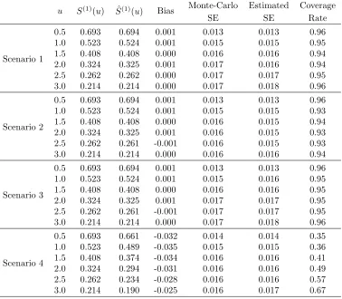
Table 1.1: Simulation 1, AIPWCC estimator for ˆS(1)(u) at selected time points when there is no stratified sampling. Sample size N=2000. Scenario 1 corresponds to “correct-correct” case; scenario 2 corresponds to“wrong propensity, correct regression” case; scenario 3 corresponds to“correct propensity, wrong regression” case; scenario 4 corresponds to“wrong propensity, wrong regression” case.

u S(1)(u) Sˆ(1)₍_u₎ _Bias Monte-Carlo Estimated Coverage

SE SE Rate

Scenario 1

0.5 0.693 0.694 0.001 0.013 0.013 0.96 1.0 0.523 0.524 0.001 0.015 0.015 0.95 1.5 0.408 0.408 0.000 0.016 0.016 0.94 2.0 0.324 0.325 0.001 0.017 0.016 0.94 2.5 0.262 0.262 0.000 0.017 0.017 0.95 3.0 0.214 0.214 0.000 0.017 0.018 0.96

Scenario 2

0.5 0.693 0.694 0.001 0.013 0.013 0.96 1.0 0.523 0.524 0.001 0.015 0.015 0.93 1.5 0.408 0.408 0.000 0.016 0.015 0.94 2.0 0.324 0.325 0.001 0.016 0.015 0.93 2.5 0.262 0.261 -0.001 0.016 0.015 0.93 3.0 0.214 0.214 0.000 0.016 0.016 0.94

Scenario 3

0.5 0.693 0.694 0.001 0.013 0.013 0.96 1.0 0.523 0.524 0.001 0.015 0.016 0.95 1.5 0.408 0.408 0.000 0.016 0.016 0.95 2.0 0.324 0.325 0.001 0.017 0.017 0.95 2.5 0.262 0.261 -0.001 0.017 0.017 0.95 3.0 0.214 0.214 0.000 0.017 0.018 0.96

Scenario 4

0.5 0.693 0.661 -0.032 0.014 0.014 0.35 1.0 0.523 0.489 -0.035 0.015 0.015 0.36 1.5 0.408 0.374 -0.034 0.016 0.016 0.41 2.0 0.324 0.294 -0.031 0.016 0.016 0.49 2.5 0.262 0.234 -0.028 0.016 0.016 0.57 3.0 0.214 0.190 -0.025 0.016 0.017 0.67

In Table 1.1, we present results for estimating the treatment-specific survival distribution

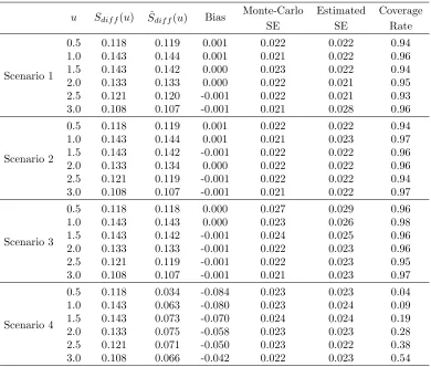
for treatment 1, S(1)(u). Results regarding the difference between two treatments Sdif f(u) are

(21)

in (1.4) is indeed consistent as desired. For scenarios 2 and 3, even though parts of the models

(propensity models/regression model) are not correctly specified, the resulting estimator is still consistent. This illustrates the doubly-robustness property. In scenario 4, the estimator is biased

as is expected because the models π(X) and H(1)(u, X) are misspecified. The coverage rate is calculated using the 95% confidence interval derived as the estimator plus/minus 1.96 estimated standard errors using the sandwich variance formulas for the four scenarios. Because in scenario

4, the estimator ˆS(1)(u) is not consistent, the coverage rate is far below 0.95. In theory, the estimated variance in scenario 3 may be conservative however, as expected, the coverage rate was close to the nominal rate of 0.95.

Note that the coverage rate in scenario 2 did not achieve the 0.95 nominal rate. This indeed

is the scenario discussed at the end of Section 1.3 where the sandwich variance estimator is not expected to be consistent. For this scenario we also estimated the asymptotic variance

and the coverage rate of the confidence interval using a nonparametric bootstrap sampling.

We used 100 bootstrap replicates and compared the bootstrap standard error with the Monte-Carlo standard error. As shown in Table 1.3, the bootstrap standard error provides an accurate

estimator of the standard error and the corresponding confidence interval computed as the

estimator plus/minus 1.96 bootstrap standard error attains the nominal coverage. This suggests that, despite of computation intensity, bootstrap variance estimator is close to the Monte-Carlo

variance and may be used in the cases when coarsening probabilities could not be estimated consistently.

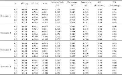
For the interest of smaller sample size performance, a simulation study with sample size

N = 200 is conducted. The data generating mechanism and parameter values remain the same. The AIPWCC estimator is computed in all four scenarios as before. Table 1.4 gives the summary

results of biasedness and standard error estimates at several time points, suggesting that the

treatment-specific survival distribution S(1)(u) can still be estimated consistently even with smaller sample size. The proposed standard error estimator, on the other hand, tends to be

unstable especially at the tail of the curve. The bootstrap standard error estimator performs

better and hence is preferable for such a smaller sample size.

Other competing estimators were also considered: the inverse probability weighted

estima-tor, the outcome regression estimator and the treatment-specific Kaplan-Meier estimator. The

numerical results can be found in Appendix D. When correctly specified, the first two estimators are consistent. The proposed AIPWCC estimator is more efficient than the inverse probability

weighted estimator and slightly less efficient than the outcome regression estimator. On the

other hand, both of these competing estimators are biased if the models are misspecified. The unadjusted treatment-specific Kaplan-Meier estimator is always biased as it does not account

(22)

1.6 Conclusion and Discussion

Viewing censored survival data from an observational study as monotonely coarsened versions

of treatment-specific potential survival times, we were able to use the powerful semiparametric theory for missing data to derive doubly robust estimators for the underlying treatment-specific

survival distributions as well as the difference in these treatment-specific distributions. We also

derived an estimator for the asymptotic variance of these estimators. Using simulation studies we demonstrated that the large sample properties of these estimators and corresponding confidence

(23)

Table 1.2: Simulation 1, AIPWCC estimator forSdif f(u) at selected time points when there is

no stratified sampling. Sample size N=2000. Scenario 1 corresponds to “correct-correct” case; scenario 2 corresponds to“wrong propensity, correct regression” case; scenario 3 corresponds to“correct propensity, wrong regression” case; scenario 4 corresponds to“wrong propensity, wrong regression” case.

u Sdif f(u) Sˆdif f(u) Bias

Monte-Carlo Estimated Coverage

SE SE Rate

Scenario 1

0.5 0.118 0.119 0.001 0.022 0.022 0.94

1.0 0.143 0.144 0.001 0.021 0.022 0.96

1.5 0.143 0.142 0.000 0.023 0.022 0.94

2.0 0.133 0.133 0.000 0.022 0.021 0.95

2.5 0.121 0.120 -0.001 0.022 0.021 0.93 3.0 0.108 0.107 -0.001 0.021 0.028 0.96

Scenario 2

0.5 0.118 0.119 0.001 0.022 0.022 0.94

1.0 0.143 0.144 0.001 0.021 0.023 0.97

1.5 0.143 0.142 -0.001 0.022 0.022 0.96

2.0 0.133 0.134 0.000 0.022 0.022 0.96

2.5 0.121 0.119 -0.001 0.022 0.022 0.94 3.0 0.108 0.107 -0.001 0.021 0.022 0.97

Scenario 3

0.5 0.118 0.118 0.000 0.027 0.029 0.96

1.0 0.143 0.143 0.000 0.023 0.026 0.98

1.5 0.143 0.142 -0.001 0.024 0.025 0.96 2.0 0.133 0.133 -0.001 0.022 0.023 0.96 2.5 0.121 0.119 -0.001 0.022 0.023 0.95 3.0 0.108 0.107 -0.001 0.021 0.023 0.97

Scenario 4

(24)

Table 1.3: Simulation 1, AIPWCC estimator forS(1)₍_u_{) at selected time points when there is no} stratified sampling. Sample size N=2000. Bootstrap inference for scenario 2, that is, the “wrong propensity, correct regression” case where variance estimator (1.5) is no longer valid. Bootstrap replicate=100.

u S(1)₍_u₎ _S_ˆ(1)₍_u₎ _Bias Monte-Carlo Bootstrap Coverage

SE SE Rate

Scenario 2

0.5 0.693 0.694 0.001 0.013 0.013 0.96 1.0 0.523 0.524 0.001 0.015 0.015 0.94 1.5 0.408 0.408 0.000 0.016 0.016 0.95 2.0 0.324 0.325 0.000 0.016 0.016 0.95 2.5 0.262 0.261 -0.001 0.016 0.016 0.94 3.0 0.214 0.214 0.000 0.016 0.017 0.95

Table 1.4: Simulation 1, AIPWCC estimator for ˆS(1)(u) at selected time points when there is no stratified sampling. Sample size N=200. Scenario 1 corresponds to “correct-correct” case; scenario 2 corresponds to“wrong propensity, correct regression” case; scenario 3 corresponds to“correct propensity, wrong regression” case; scenario 4 corresponds to“wrong propensity, wrong regression” case. Bootstrap replicate=500.

u S(1)(u) Sˆ(1)(u) Bias Monte-Carlo Estimated Bootstrap CR CR SE SE SE (Proposed) (Bootstrap)

Scenario 1

0.5 0.693 0.696 0.003 0.039 0.041 0.042 0.95 0.96 1.0 0.523 0.524 0.001 0.049 0.048 0.049 0.94 0.94 1.5 0.408 0.410 0.002 0.050 0.051 0.052 0.95 0.95 2.0 0.324 0.326 0.001 0.051 0.052 0.054 0.95 0.95 2.5 0.262 0.259 -0.003 0.054 0.053 0.056 0.92 0.93 3.0 0.214 0.203 -0.012 0.061 0.054 0.067 0.89 0.95

Scenario 2

0.5 0.693 0.697 0.003 0.039 0.042 0.041 0.96 0.96 1.0 0.523 0.524 0.001 0.048 0.046 0.048 0.93 0.94 1.5 0.408 0.411 0.003 0.048 0.048 0.051 0.94 0.95 2.0 0.324 0.326 0.002 0.050 0.048 0.052 0.94 0.95 2.5 0.262 0.260 -0.002 0.052 0.048 0.054 0.91 0.93 3.0 0.214 0.205 -0.009 0.059 0.049 0.060 0.86 0.94

Scenario 3

0.5 0.693 0.696 0.003 0.039 0.042 0.042 0.96 0.95 1.0 0.523 0.524 0.000 0.049 0.049 0.049 0.95 0.94 1.5 0.408 0.410 0.002 0.050 0.052 0.052 0.96 0.95 2.0 0.324 0.326 0.001 0.051 0.053 0.054 0.95 0.96 2.5 0.262 0.259 -0.003 0.054 0.054 0.056 0.93 0.94 3.0 0.214 0.203 -0.011 0.062 0.055 0.067 0.89 0.94

Scenario 4

(25)

Chapter 2

Doubly-robust Estimators of

Survival Distributions in Stratify

Sampled Observational Studies with

Additional Information from a

Subsample

2.1 Introduction

In Chapter 1, we derive doubly robust estimators (and their asymptotic variance) of the

treatment-specific survival distributions and the difference in the treatment-specific survival distributions in the case when the collected covariates are enough to adjust for all confounding

in the main study by using the semiparametric theory for missing data. However, it is important

to keep in mind that the consistency of previously derived estimator depends on the crucial no unmeasured confounder assumption that all potential confounders are captured, which in

reality may not true.

This is indeed the case in a data example known as the ASCERT study, an observational study funded by the National Heart Lung and Blood Institute to compare two widely used

treatment options for patients with coronary artery disease (Weintraub et al., 2012), where the

investigators had concerns about the possibility of residual confoundings. The ASCERT study was a retrospective analysis patients who had either two-vessel or three-vessel coronary artery

disease and were treated either by surgical revascularization (coronary artery bypass grafting;

(26)

patients were followed until the endpoint of interest (all-cause mortality); accordingly, survival

outcomes for these patients were censored. Moreover the investigators recognized that assess-ment of coronary anatomy was limited to a few relatively crude variables. For example, patients

with certain high-risk coronary features may have been preferentially selected for CABG over

PCI. To address this limitation, a sub-study was conducted in which detailed data on coro-nary anatomy were collected on a stratified random sample of patients at 54 hospitals in the

main ASCERT study. According to the protocol, approximately 500 patient records were to

be randomly selected without replacement from each of four strata formed by all combinations of the two treatments and whether or not the patients had two- or three-vessel disease. For

each randomly selected patient, X-ray films of coronary angiograms taken prior to the patient’s

revascularization procedure were retrieved from storage and sent to a central laboratory for expert interpretation and analysis. More details of this study are given in Section 2.6.

The challenge is that of acknowledging this design in the comparison of treatment-specific

survival distributions. There is a vast literature on methods for incorporating data from a subsample into such analyses (e.g., Breslow and Cain, 1988; Flanders and Greenland, 1991;

Zhao and Lipsitz, 1992; Mark and Katki, 2006; St¨urmer et al., 2007, and references therein).

However, to our knowledge, there is no work applicable to a setting like that of ASCERT to develop estimators for survival distributions that take full advantage of the data collected

on the entire cohort to achieve the greatest efficiency possible and that possess the double robustness property to protect against model misspecification. Currently, theory for AIPWCC

estimators is based on the assumption that observations across subjects are independent and

identically distributed (iid), which is clearly not the case for data collected according to a stratified sampling scheme.

In this chapter, we develop estimators for survival distribution in the case when a stratified

sampling substudy is further conducted in order to collect additional potential confounding covariates.

2.2 Notations and Assumptions

Let Vi = (Ui,∆i, Zi, X1i), i = 1, . . . , N denote the data available on all subjects in the main

study, where nowX1 represents covariates collected on these subjects. The key requirement for using the previously proposed method is the strong ignorability assumption, which here would

(27)

subjects in stratumk, k= 1, . . . , K, then from stratumk, a fixed (by design) number of subjects

nk are sampled from the Nk subjects at random without replacement. For each subject so

included in the substudy, additional covariatesX2are collected, where, lettingX = (X1T, X2T)T, it is believed that the strong ignorability assumption Z ⊥⊥T(j)|X holds. Let Ri = 1 if subject i= 1, . . . , N, was selected into the subsample and 0 otherwise. The goal is to estimate S(1)(u) (andSdif f(u)) using the observed data Oi= (Ui,∆i, Zi, X1i, Ri, RiX2i)

2.3 Inference for Treatment-specific Survival Distributions

Again, here we use the missing data analogy. We identify the “full data” that would ideally have

been collected on all N subjects as Fi = (Ui,∆i, Zi, X1i, X2i), i = 1, . . . , N, recognizing that X2 is collected only on subjects in the substudy. Were there full data available, a consistent, asymptotically normal, doubly robust estimator forS(1)₍_u_{) could be found by solving}

N

X

i=1

φ{Fi, S(1)(u)}= 0

, whereφ{F, S(1)(u)}is the estimating function (1.3). We may identify the observed data as full data withX2 missing for subjects not selected in the subsample. Accordingly, following Tsiatis (2006), we propose the class of AIPWCC estimators defined as the solution to

N

X

i=1 "

Riφ{Fi, S(1)(u)} η(i)

−

Ri−η(i) η(i)

h(Vi)

#

= 0, (2.1)

where η(i) = P(Ri = 1|i), taking values nk/Nk when i = k, the probability of selection

into the subsample as a function of the stratum to which subject i belongs; and h(Vi) is an

arbitrary function of the data collected on all subjects. Here, if we set h(Vi) = 0, then the

resulting estimator is a simple inverse probability weighted estimator, which we refer to as

the weighted estimator. However, the choice of h(V) will affect the asymptotic variance of the resulting estimator.

The usual theory for AIPWCC estimators applies when the observed data Oi, i= 1, . . . , N,

are iid. We briefly outline our proposed modification to account for the stratified sampling.

Rear-ranging (2.1), we write this estimating equation asT{O, S(1)(u)}= 0, whereO= (O1, . . . , On)

(all the observed data) and

T{O, S(1)(u)}=

K

X

k=1

Nk N

P

i:i=kRi[φ{Fi, S

(1)₍_u₎_{} −}_h₍_V

i)] nk

+ P

i:i=kh(Vi)

Nk

!

(28)

Letting µk(φ) = E[φ{F, S(1)(u)}| = k] and µk(h) = E[h(V)| = k], it is straightforward to

observe that

E[T{O, S(1)(u)}] = E(E[T{O, S(1)(u)}|N1, . . . , NK])

= E[

K

X

k=1

(Nk/N){µk(φ)−µk(h) +µk(h)}]

=

K

X

k=1

pkµk(φ)

= E[φ{F, S(1)(u)}],

where pk = P( = k). This implies that T{O, S(1)(u)} is an unbiased estimating function.

Consequently, the solution to (2.1) will yield an estimator for S(1)(u) which will converge in limit to the same estimand as the solution to the full data estimating equation given by (1.3) with X = (XT

1, X2T)T. In particular, this means that the proposed AIPWCC estimator will have the double robustness property as described in the previous section. This result is true

regardless of the choice forh(V).

To derive the optimal choice ofh(V) and to support large sample inference, we must derive

the asymptotic variance of estimators solving (2.1) and an estimator for the asymptotic variance

of T{O, S(1)(u)}. Note that

Var[T{O, S(1)(u)}] =E(Var[T{O, S(1)(u)}|N1, . . . , NK]) + Var(E[T{O, S(1)(u)}|N1, . . . , NK]).

We showed above that

E[T{O, S(1)(u)}|N1, . . . , NK]) = K

X

k=1

Nk N µk(φ),

which, because (N1, . . . , NK) is multinomial (N;p1, . . . , pK), implies

Var(E[T{O, S(1)(u)}|N1, . . . , NK]) =N−1

 

K

X

k=1

pkµ2k(φ)−

( _K X

k=1

pkµk(φ)

)2

. (2.3)

Because the data from the nk and Nk−nk individuals in stratumk who were selected or not

in the subsample are independent realizations from the population in stratum k, and because

(29)

that Var[T{O, S(1)(u)}|N1, . . . , NK] equals K X k=1 Nk N 2

{Vark(φ)−2Covk(φ, h) + Vark(h)}

1 nk − 1 Nk

+ Vark(φ)

1

Nk

, (2.4)

where Vark(φ) = Var[φ{F, S(1)(u)}| = k],Vark(h) = Var{h(V)| = k}, and Covk(φ, h) =

Cov[φ{F, S(1)(u)}, h(V)|=k]. Thus Var[T{O, S(1)(u)}] is given by (3.5) plus the expectation of (2.4), and the function h(V) that minimizes this variance is obtained by minimizing (2.4).

Because

{Vark(φ)−2Covk(φ, h) + Vark(h)}= Var[φ{F, S(1)(u)} −h(V)|=k],

it is straightforward to show that the optimal choice is

hopt(V) =E[φ{F, S(1)(u)}|V],

which, although is a function ofV, we write as

hopt(V) =E[φ{F, S(1)(u)}|V, ] =

K

X

k=1

I(=k)E[φ{F, S(1)(u)}|V, =k]

to emphasize that the best choice for h(V) in each summand of (2.2) is the conditional

expec-tation of φ{F, S(1)(u)} givenV within each stratum.

If we write φ{F, S(1)(u)} of equation (1.3) asφ∗₁(F)−S(1)(u), where φ∗₁(F) equals

ZI(U ≥u)

π(X)Kc(1)(u, X)

−

Z−π(X)

π(X)

H(1)(u, X) + Z u

0

Z π(X)

dMc(1)(r, X)

Kc(1)(r, X)

(

H(1)(u, X)

H(1)₍_{r, X}₎ )

, (2.5)

then after some algebra, we can show that the optimal estimator forS(1)(u) is given by

ˆ

S_strat(1) (u) =N−1 N

X

i=1

Riφ∗1(Fi) η(i)

−

Ri−η(i) η(i)

E{φ∗₁(Fi)|Vi, i}

, (2.6)

whereE{φ∗₁(Fi)|Vi, i}=PKk=1I(i =k)E{φ∗1(Fi)|Vi, i =k}.

As the conditional expectationE{φ∗₁(F)|V, =k}are not known, we would propose models

wk(V, ψ_k(1)) for them in terms of parametersψ(1)_k . The ψ(1)_k may be estimated via least squares

as follows using the data on subjects in the subsample from stratum k (where both F and V

are collected). For each subject i in the subsample, form an estimator ˆφ∗₁_i, say, for φ∗₁(Fi) as

(30)

estimator ˆψ(1)_k is derived by minimizingP

i:Ri=1,i=k{

ˆ

φ∗₁_i−wk(Vi, ψ_k(1))}2 inψ(1)_k . The estimator

for S(1) _{is the solution to equation (2.6) with} _E_{_φ∗

1(Fi)|Vi, i} replaced by wk(Vi,ψˆ_k(1)) when i=k.

Care must be taken in estimatingπ(X), H(1)(r, X) andKc(1)(r, X), as all variables inX are

collected only on subjects in the subsample. BecauseH(1)₍_{r, X}_{) and}_K(1)

c (r, X) are probabilities

conditional on X and Z = 1, and because the strata are defined through X1 (the subset of X observed for all subjects) and Z, consistent estimators for these functions may be derived by modeling and fitting based on the subsample in a manner analogous to that based the entire

sample when there is no stratified sampling. However, this is not the case for the propensity

scoreπ(X). For the sake of clarity, suppose as in ASCERT that theK = 2M strata are defined by all combinations ofM categories derived through components ofX1 and the two treatment levels 0 and 1. Denote the number of subjects in the stratum corresponding to them-th category

for treatments 1 and 0 as N1m and N0m and the corresponding numbers in the subsample as n1mandn0m, respectively,m= 1, . . . , M. Then, using redundant notation similar to that above

and letting Cat be the indicator for category, it is straightforward to show that if

logit{P(Z = 1|X, Cat=m)}=ζ(X, m),

then

logit{P(Z = 1|X, Cat=m, R= 1)}=ζ(X, m) + log(n1m/N1m)−log(n0m/N0m),

where logit(θ) = log{θ/(1−θ)}. Consequently, writing

π(X) =

M

X

m=1

I(Cat=m)π(X, m),

where π(X, m) = P(Z = 1|X, Cat = m), we propose estimating π(X) by fitting postulated models for each π(X, m). This may be based on fitting logistic regression models to the sub-sample data (Zi, Xi), i:Ri= 1 of the form

logit{P(Z = 1|X, Cat=m, R= 1)}=ζ∗(X, m),

so that the estimator for π(X, m) is of the form

expit{ζ∗(X, m)−log(n1m/N1m) + log(n0m/N0m)},

where expit(θ) =eθ/(1 +eθ).

(31)

additional covariate informationX2 was not predictive forπ(X),Kc(1)(r, X) orH(1)(r, X), then E{φ∗₁(F)|V, = k} = φ∗₁(V). Of course, this is generally not the case but this suggests that we might consider a model where we assume that E{φ∗₁(F)|V, = k] = ψ(1)₀_k +ψ₁(1)_kφ∗₁(V). Keep in mind that we will obtain a doubly robust estimator for S(1)(u) regardless of whether or not the model for wk(V, ψ

(1)

k ) is correctly specified. However, a good approximation for E{φ∗₁(F)|V, =k} should result in gains in efficiency. Consequently, the suggested strategy is to derive an estimated ˜φ∗₁(Vi) for individualiexactly as was suggested in Section 2 for estimating

(2.5) using all the data from the main study with only X1. The parameter ψ_k(1) is estimated using least squares by minimizing P

i:Ri=1,i=k{

ˆ

φ₁∗_i−ψ₀(1)_k −ψ₁(1)_kφ˜∗₁(Vi)}2 inψ_k(1). The resulting

AIPWCC stratified estimator is given by

ˆ

S_strat(1) (u) =N−1 N

X

i=1 "

Riφˆ∗1i η(i)

−

Ri−η(i) η(i)

{ψˆ₀(1)_k + ˆψ₁(1)_kφ˜∗₁(Vi)}

#

. (2.7)

As we will demonstrate in the simulations studies (Section 2.5), this strategy leads to an

esti-mator that has good performance.

The variance estimator for the estimator of S(1)(u) would then use (3.5) plus (2.4), substi-tuting the natural estimators forpk, µk(φ), µk(h),Vark(φ),Vark(h) and Covk(φ, h), where here

we take

h(V) =

K

X

k=1

I(=k){ψ₀(1)_k +ψ(1)₁_kφ∗₁(V)−S(1)(u)}.

As in the case when there is no stratified sampling, the double robustness property as well as the adequacy of the proposed variance estimator will depend on whether or not the models for

π(X) (used for the propensity score),Kc(1)(r, X) and H(1)(r, X) are correctly specified.

2.4 Inference on Difference of Treatments

Since we are also interested in making inference on Sdif f(u), we also provide an estimator for

Sdif f(u) and its variance estimator when a substudy is conducted. In Section 2.3, we have

shown that (2.7) is a consistent estimator of S(1)₍_u_{). Similarly, we can estimate the difference} functionSdif f(u) by

ˆ

Sdif f,strat(u) =N−1 N

X

i=1

Riφˆ∗dif f,i η(i)

−

Ri−η(i) η(i)

ˆ

h∗_{dif f}(Vi)

!

,

where ˆφ∗_{dif f,i} = ˆφ∗₁_i−φˆ∗₀_i, for treatment j = (0,1), ˆφ∗_{j i} is the estimator for φ∗_j(Fi) defined by

equation (1.6) withXi = (X1Ti, X2Ti)T, and ˆh∗dif f(Vi) ={ψˆ0(1)k + ˆψ

(1)

1kφ˜∗1(Vi)} − {ψˆ(0)0k + ˆψ

(0)

(32)

where ˆψ_k(j)is obtained using least squares by minimizingP

i:Ri=1,i=k{

ˆ

φ_{j i}∗ −ψ₀(j_k)−ψ₁(j_k)φ˜∗_j(Vi)}2, j= 0,1. The asymptotic variance can be estimated by substituting the above ˆφ∗_{dif f} and ˆhdif f(V)

into (3.5) and (2.4).

2.5 Simulations

In this simulation we consider the case where we conduct a substudy using stratified sam-pling and consider the performance of our stratified AIPWCC estimators. Using the same data

generating mechanism as in Section 1.5, we collected X1 on the main study of N = 5,000 observations and randomly sampled n11 = n12 = n01 = n02 = 300 observations from each of

K = 4 stratum combination of (Z, B) without replacement and collected additional covariates

X2 on these subsamples. In these simulations we used the correct models forπ(X),Kc(j)(r, X),

and H(j)(r, X),j= 0,1.

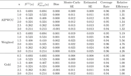
We compared the consistency and efficiency of three estimators forS(1)(u) under this setting. The first estimator is the estimator (2.7). We refer to this estimator as the AIPWCC stratified

estimator. The second one used the estimator resulting from (2.1), where the augmentation term

h(Vi) = 0, referred to as theweighted estimator. We also considered the infeasible estimator (1.4)

with covariates X1, X2 on the whole dataset as the gold standard.

As expected, all three estimators along with their estimated standard errors are consistent and the confidence intervals have coverage rate close to the nominal rate of 0.95.

The relative efficiency is computed by taking the ratio of the Monte-Carlo variance of each estimator over the Monte-Carlo variance of the gold standard estimator. Here we see the large

gains in efficiency using the AIPWCC stratified estimator compared to the weighted estimator

with little loss of efficiency compared to the gold standard. Recall that the weighted estimator only uses data from the substudy whereas theAIPWCC stratified estimatoruses all the observed

data.

This illustrates that choosing the augmentation term appropriately can recover a great deal of information from the main study and result in large gains in efficiency.

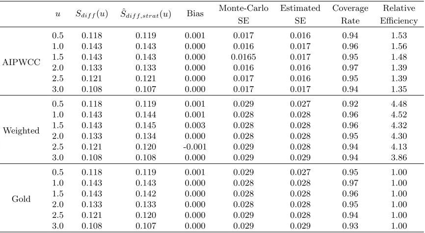
We also compared the performance of estimator forSdif f(u) (see Table 2.2) and the results

are similar to the above estimators of S(1)(u). In addition, we conducted simulation studies where the models for either the propensity scoreπ(X) or the conditional survival distribution

(33)

Table 2.1: Simulation 2, estimators for ˆS_strat(1) (u) at selected time points when there is subsample to collect additional covariates. Sample size N=5000, n11 = n12 = n01 = n02 = 300 samples randomly selected from K=4 strata. The relative efficiency (RE) is the ratio of Monte-Carlo variance of each estimator over the Monte-Carlo variance of the gold standard estimator.

u S(1)₍_u₎ _S_ˆ(1)

strat(u) Bias

Monte-Carlo Estimated Coverage Relative

SE SE Rate Efficiency

AIPWCC

0.5 0.693 0.694 0.000 0.009 0.009 0.96 1.20

1.0 0.523 0.523 0.000 0.011 0.011 0.95 1.31

1.5 0.408 0.408 0.000 0.012 0.012 0.95 1.36

2.0 0.324 0.324 0.000 0.012 0.012 0.95 1.34

2.5 0.262 0.262 0.000 0.013 0.013 0.95 1.37

3.0 0.214 0.213 -0.001 0.013 0.013 0.94 1.32

Weighted

0.5 0.693 0.694 0.001 0.019 0.019 0.95 5.19

1.0 0.523 0.524 0.001 0.021 0.021 0.96 5.10

1.5 0.408 0.410 0.002 0.023 0.023 0.94 5.56

2.0 0.324 0.325 0.001 0.022 0.023 0.96 4.76

2.5 0.262 0.262 0.000 0.023 0.024 0.96 4.46

3.0 0.214 0.214 0.000 0.024 0.025 0.96 4.26

Gold

0.5 0.693 0.693 0.000 0.008 0.008 0.95 1.00

1.0 0.523 0.523 0.000 0.009 0.010 0.95 1.00

1.5 0.408 0.407 0.001 0.010 0.010 0.94 1.00

2.0 0.324 0.324 0.000 0.010 0.010 0.96 1.00

2.5 0.262 0.261 -0.001 0.011 0.011 0.94 1.00

3.0 0.214 0.214 0.000 0.012 0.011 0.94 1.00

2.6 Analysis of the ASCERT Study

In this section, we apply the proposed AIPWCC estimator to data from the ASCERT study.

The goal of the analysis was to estimate the AIPWCC-adjusted 4-year survival distribution for PCI and CABG using baseline covariate data from the main ASCERT study database

augmented with information on coronary anatomy from a subsample of patients in the ASCERT

angiographic companion study. The sampling frame consisted of records from 9,800 patients in the ASCERT database who underwent a coronary revascularization procedure (CABG or

PCI) at one of 54 hospitals participating in the ASCERT study that agreed to be part of

the companion study. For the purpose of this analysis we considered the patients from the 54 hospitals of the companion study to be the main focus of inference. Eighteen covariates

were used on the full sample which included demographics (e.g., age, sex), risk factors (e.g.,

(34)

Table 2.2: Simulation 2, estimators for ˆSdif f,strat(u) at selected time points when there is

sub-sample to collect additional covariates. Sample size N=5000, n11 = n12 = n01 = n02 = 300 samples randomly selected from K=4 strata. The relative efficiency (RE) is the ratio of Monte-Carlo variance of each estimator over the Monte-Monte-Carlo variance of the gold standard estimator.

u Sdif f(u) Sˆdif f,strat(u) Bias

Monte-Carlo Estimated Coverage Relative

SE SE Rate Efficiency

AIPWCC

0.5 0.118 0.119 0.001 0.017 0.016 0.94 1.53

1.0 0.143 0.143 0.000 0.016 0.017 0.96 1.56

1.5 0.143 0.143 0.000 0.0165 0.017 0.95 1.48

2.0 0.133 0.133 0.000 0.016 0.016 0.97 1.39

2.5 0.121 0.121 0.000 0.017 0.016 0.95 1.39

3.0 0.108 0.107 0.000 0.017 0.017 0.94 1.35

Weighted

0.5 0.118 0.119 0.001 0.029 0.027 0.92 4.48

1.0 0.143 0.144 0.001 0.028 0.028 0.96 4.52

1.5 0.143 0.145 0.003 0.028 0.028 0.96 4.32

2.0 0.133 0.134 0.000 0.028 0.028 0.95 4.30

2.5 0.121 0.120 -0.001 0.029 0.028 0.94 4.13

3.0 0.108 0.108 0.000 0.029 0.029 0.94 3.86

Gold

0.5 0.118 0.119 0.001 0.029 0.027 0.95 1.00

1.0 0.143 0.143 0.000 0.028 0.028 0.97 1.00

1.5 0.143 0.142 0.000 0.028 0.028 0.96 1.00

2.0 0.133 0.133 0.000 0.028 0.028 0.95 1.00

2.5 0.121 0.120 0.000 0.029 0.028 0.94 1.00

3.0 0.108 0.107 0.000 0.029 0.029 0.93 1.00

from approximately 2,000 patients chosen by design (roughly 500 in each of the four strata

determined by all combinations of the two treatments and whether or not the patients had two- or three-vessel disease). Information collected on the subsample includes features of the

patient’s coronary anatomy (e.g., left-side dominance) and features of each individual blockage

(e.g., lesion length, tortuosity, calcification, degree of stenosis).

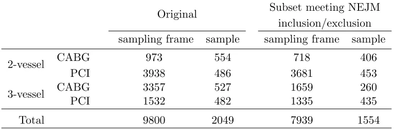
The original sampling frame comprised 9,800 patients. Subsequently it was determined that

some patients were ineligible for analysis. Consequently, the main study participants consisted

of 7,393 eligible patients among the 9,800 patients in the 54 hospitals of the companion study and the subsample consisted of 1,554 eligible patients among the 2,049 originally sampled.

Table 2.3 provides details on the sample size before and after eligibility was determined.

Figure 2.1 presents plots of the estimated AIPWCC-adjusted survival distributions with accompanying 95% pointwise confidence intervals for PCI, CABG and their difference as

es-timated by the proposed AIPWCC estimator. Overall, results are highly consistent with the published primary ASCERT analysis (Weintraub et al., 2012). Short-term risk appears to be

(35)

Table 2.3: Number of Patients in the Sampling Frame and Sample.

Original Subset meeting NEJM

inclusion/exclusion sampling frame sample sampling frame sample

2-vessel CABG 973 554 718 406

PCI 3938 486 3681 453

3-vessel CABG 3357 527 1659 260

PCI 1532 482 1335 435

Total 9800 2049 7939 1554

Table 2.4 presents the estimated AIPWCC-adjusted cumulative incidence (one minus the

survival distribution) of mortality at two time points (30 days and 4 years) and compares two

versions of the adjusted analysis together with the unadjusted treatment-specific Kaplan-Meier estimators. The first AIPWCC estimator adjusts only for covariates available in the full sample

and includes all 7,393 patients. The second analysis used the AIPWCC stratified estimator

and includes the additional covariates on coronary anatomy collected on the subsample and corresponds to the analysis shown in Figure 2.1. In each case, the 30-day estimate favors PCI

whereas the 4-year estimate favors CABG. Both adjusted analyses gave similar results with

possibly CABG having slightly better performance compared to PCI in the unadjusted analysis. Overall all three analyses gave similar results suggesting that the confounding, either with

covariates used in the main study or those collected in the substudy, was not substantial.

2.7 Conclusion and Discussion

The AIPWCC estimator derived in chapter 1 provide valid inference if the key assumption of no

unmeasured confounder holds. In the case when additional covariate information is necessary to make the assumption of no unmeasured confounders tenable, we could conduct a substudy

using a stratified sampling design to collect such additional covariates and we have proposed

a method for obtaining doubly robust estimators with such a design which uses the data from the main study to gain efficiency. The corresponding estimator and standard error estimator

(36)

0 1 2 3 4

80

85

90

95

100

Years from Procedure

Sur

viv

al (%)

CABG

PCI

A. Survival

0 1 2 3 4

−5

0

5

Years from Procedure

Diff

erence in Sur

viv

al (%)

B. Difference in Survival

(37)

Table 2.4: Estimated AIPWCC-Adjusted Cumulative Incidence of Mortality at 30 Days and 4 Years by Treatment Group, Expressed as Percentage With 95% Confidence Interval. The proposed standard error estimator is used to compute the confidence interval.

30-day (%) 4-year (%)

CABG 1.77 ( 1.24, 2.30) 14.69 (12.90, 16.49) Unadjusted Kaplan Meier PCI 1.14 ( 0.84, 1.43) 18.64 (17.25, 20.03) Difference -0.64 (-1.24, -0.03) 3.95 ( 1.68, 6.22)

CABG 2.17 ( 1.50, 2.83) 15.93 (13.98, 17.88) AIPWCC (Full) PCI 1.08 ( 0.79, 1.38) 18.31 (16.95, 19.67) Difference -1.08 (-1.81, -0.36) 2.38 ( 0.04, 4.73)

(38)

Chapter 3

A Doubly-Robust Log Rank Type

Test for Comparing Survival

Distributions in an Observational

Study With and Without an

Auxiliary Substudy

3.1 Introduction

Besides treatment-specific survival curve estimates discussed in the previous two chapters, the

overall comparison of treatment-specific survival distributions is also an important issue in sur-vival analysis. In a randomized controlled clinical trial where covariate distribution is balanced

among different treatment groups, the log rank test is most commonly used to test the null

hypothesis that there is no significant difference between treatments. In an observational study, however, the traditional log rank test is no longer valid due to possible confounding.

Xie and Liu (2005) proposed an inverse probability weighted log rank test to adjust for such

confounding. They computed a weighted version of log rank statistics by substituting inverse probability weighted number of subject at risk and number of subject that die in each group.

This estimator would provide valid inference if the propensity model is consistently estimated.

Zhang and Schaubel (2012) compared treatment groups in term of the difference in restricted mean lifetime, which they referred as the average causal effect. This is a semiparametric

estima-tor with a doubly-robust property. However, its consistency relies on the underlying assumption

(39)

covariates also have effect on censoring which may likely be the case in observational studies,

this method might be subject to bias.

In this chapter, we propose a log rank type test statistics to compare treatment groups.

With a nonparametric bootstrap estimator of the denominator, the resulting test statistics will

be doubly-robust. Moreover, we generalize the statistics into the case where a substudy is to be conducted to collect additional covariates as discussed in Chapter 2 to account for residual

confounding.

3.2 Test Statistic for Main Study when all Potential Confounders

are Captured

In this section, we develop the log rank type statistic when the covariates collected in the main study are believed to capture all potential confounding. The assumptions are the same as those

described in Chapter 1 where we developed the doubly-robust estimator for treatment-specific

distributions S(j)(u) =P(T(1) ≥u), u≥0, j = 0,1 as

ˆ

S(j)(u)=N−1 N

X

i=1

φ∗_j(u;Vi)

=N−1 N

X

i=1 "

(Zi)j(1−Zi)1−jI(Ui≥u)

{π(Xi)}j{1−π(Xi)}1−jKc(j)(u, Xi)

− (2j−1){Zi−π(Xi)} {π(Xi)}j{1−π(Xi)}1−j

H(j)(u, Xi)

+ Z u

0

(Zi)j(1−Zi)1−j

{π(Xi)}j{1−π(Xi)}1−j

dMc(j)(r, Xi)

Kc(j)(r, Xi)

H(j)(u, Xi) H(j)₍_{r, X}

i)

#

, (3.1)

where π(X) = P(Z = 1|X) is the propensity score, Kc(j)(r, X) = P(C ≥ r|X, Z = j) is the

conditional survival function of the treatment specific censoring time given X, dMc(j)(r, X)

is the martingale increment for the censoring distribution, namely, dMc(j)(r, X) = dNc(r)− λ(cj)(r, X)Y(r), Nc(r) =I(U ≤r,∆ = 0), Y(r) = I(U ≥ r) and λ(cj)(r, X) = −d logK

(j)

c (r,X)

dr is

the conditional hazard function forC givenZ =j and X, and H(j)(r, X) =P(T(j)≥r|X). In Chapter 1 we also derived the estimator ˆS(1)(u)−Sˆ(0)(u) and its variance estimator allowing us to compare the survival distributions at a fixed time point u.

The treatment comparison of the overall survival distributions is often of interest and is commonly based on estimating the treatment-specific hazard ratio assuming a proportional

hazards model. That is, we assumeλ(1)(u) =λ(0)(u) exp(α), whereλ(j)(u) = limh→0h−1P(u≤

T(j)< u+h|T(j)≥u) is the hazard function ofT(j) at time u,j = 0,1. The log hazard ratio

α is then of interest.