ABSTRACT
FINNEGAN, PETER CHARLES. Enhanced CO2 Detection and H2O Quantification with
both a Thermoelectrically Cooled Spectrometer and a Fourier Transform Infrared (FTIR) Spectrometer. (Under the direction of Dr. Alexei V. Saveliev.)
The current state of power generation systems has changed as the fuel sources content and heating value have become more variable. Producer gas, landfill gas and syngas are a few examples of fuel sources which are becoming more prevalent today. These opportunity fuels vary in composition and heating value depending on the geographic location, among other factors. Gas chromatography (GC) has become the industry standard for measuring fuel composition; however, this process takes time (~10 minutes), is expensive, and requires a skilled operator. The proposed work consists of utilizing near infrared (NIR) spectroscopy, along with multivariate regression methods to provide quantitative real time composition and heating content data for mixtures containing C1-C4 alkanes, CO2 and N2. These components
are common species in landfill gas, producer gas and syngas. As a major constituent in landfill gas, CO2 has weaker absorption bands in the current near infrared range compared to
C1-C4 alkanes. Thus, the accurate measurement of CO2 is a topic of importance in this
thesis. A longer wavelength near infrared mini spectrometer is utilized to recognize a distinct absorption band of CO2 in the 2 μm range. Additionally, the capability of measuring water
Enhanced CO2 Detection and H2O Quantification with both a Thermoelectrically Cooled
Spectrometer and a Fourier Transform Infrared (FTIR) Spectrometer
by
Peter Charles Finnegan
A thesis submitted to the Graduate Faculty of North Carolina State University
in partial fulfillment of the requirements for the Degree of
Master of Science
Mechanical Engineering
Raleigh, North Carolina 2014
APPROVED BY:
__________________________ Dr. Alexei Saveliev Chair of Advisory Committee
___________________________ ___________________________
Dr. Venkateswaran Narayanaswamy Dr. John Strenkowski
ii DEDICATION
iii BIOGRAPHY
iv ACKNOWLEDGEMENTS
To Dr. Saveliev, I can’t put into words how much gratitude and thanks I have for you. You honestly have been more than an advisor, and I will never forget your patience and
benevolence to me. I’d also like to thank Dr. Strenkowski and Dr. Narayanaswamy for serving on my advisory committee.
Thank you to GTI for your support during my project.
To all my new friends in Raleigh, thank you for being so welcoming. Especially Parth, Suhwan, Wei, and Gray for keeping the mood relaxed and enjoyable in the lab.
v TABLE OF CONTENTS
LIST OF TABLES ... vii
LIST OF FIGURES ... viii
1 INTRODUCTION AND BACKGROUND... 1
1.1 Opportunity fuels... 1
1.2 Conventional methods for hydrocarbon fuel mixture analysis ... 2
1.2.1 Calorimetry ... 3
1.2.2 Gas chromatography ... 4
1.3 Potential alternative methods ... 6
1.3.1 Dispersive NIR spectroscopy ... 6
1.3.2 Fourier transform infrared (FTIR) spectroscopy ... 7
1.4 A literature review of NIR spectroscopy analysis ... 9
1.4.1 Quantum mechanical model ... 9
1.4.2 Beer’s law ... 13
1.4.3 Multivariate methods ... 14
1.5 Thesis objectives ... 19
2 EXPERIMENTAL APPROACH ... 21
2.1 Optical setup ... 21
2.2 Flow control ... 23
2.3 Data acquisition system ... 25
2.4 Experimental procedures ... 26
3 EQUIPMENT SELECTION AND ACCURACY OF MEASUREMENTS ... 29
3.1 Selection of spectral range ... 29
3.1.1 Spectral convolution ... 30
3.2 Spectrometer selection ... 32
3.3 Spectral uncertainty ... 33
3.3.1 Signal-to-noise ratio ... 33
3.3.2 Selectivity and limit of detection ... 36
vi
4 ENHANCED CO2 DETECTION WITH A THERMOELECTRICALLY
COOLED SPECTROMETER TO PROVIDE BROADER SPECTRAL RANGE ... 39
4.1 Experimental validation ... 39
4.2 Results and discussion ... 41
5 WATER VAPOR QUANTIFICATION WITH A THERMOELECTRICALLY COOLED SPECTROMETER ... 44
5.1 Background ... 44
5.1.1 Psychrometrics ... 45
5.2 Experimental approach ... 47
5.2.1 Experimental equipment and setup ... 48
5.2.2 Experimental conditions ... 50
5.2.3 Results and discussion ... 52
6 A NON-DISPERSIVE SPECTRAL METHOD TO ACCURATELY PREDICT OPPORTUNITY FUEL BLENDS: MEMS-FTIR ... 56
6.1 Experimental methods ... 56
6.2 Results and discussion ... 57
CONCLUSIONS ... 61
FUTURE WORK ... 64
REFERENCES ... 65
APPENDICES ... 69
APPENDIX A1 ... 70
vii LIST OF TABLES
Table 1. Selectivity and limits of detection using 6 principal components. ... 36
Table 2. Uncertainty in flow rate and composition for each mixture component. ... 38
Table 3. Laboratory calibration and validation mixtures. ... 40
Table 4. Experimental parameters ... 51
Table 5. Experimental mixture composition and heating values. ... 51
Table 6. Prediction error for individual validation mixtures (PCR with 5 components). ... 53
viii LIST OF FIGURES
Fig. 1.1 Typical concentration of opportunity fuels. ... 2
Fig. 1.2 Diagram of a gas chromatograph [10]. ... 5
Fig. 1.3 Optical diagram of the Michelson interferometer [17]. ... 8
Fig. 1.4 Fourier transform applied to monochromatic radiation [17]. ... 9
Fig. 1.5 Photon absorption and emission. ... 10
Fig. 1.6 Diatomic oscillator model. ... 11
Fig. 1.7 Examples of (a) symmetric stretching, (b) wagging, and (c) scissoring vibrational modes. ... 12
Fig. 1.8 Using chemometrics to determine difficult to measure data. ... 15
Fig. 2.1 Experimental setup ... 21
Fig. 2.2 Optical setup of sensor ... 23
Fig. 2.3 Interface connector P6 pinout for mass flow controllers [28]. ... 24
Fig. 2.4 Hamamatsu SpecEvaluation GUI ... 26
Fig. 3.1 HITRAN high resolution spectra of CO2. ... 30
Fig. 3.2 Convoluted spectra of CO2 ... 31
Fig. 3.3 Measured spectra of carbon dioxide, methane, propane and nitrogen humidified with water vapor at 52°C and 100 % RH. ... 32
Fig. 3.4 Reference intensity measured by spectrometer (including dark subtraction). ... 33
Fig. 3.5 Noise spectra... 34
ix
Fig. 4.1 Resulting spectra of 11 calibration mixtures. ... 41
Fig. 4.2 Comparison of predicted and actual composition and heating value for (a) C3H8, (b) CO2, (c) CH4, and (d) mixture heating content. ... 42
Fig. 4.3 Variance explained by each PLS component. ... 43
Fig. 5.1 Simulated spectra consisting of convoluted HITRAN data... 45
Fig. 5.2 Water vapor quantification experimental diagram. ... 47
Fig. 5.3 Experimental setup ... 48
Fig. 5.4 Omega CN77532-A2 temperature controller pin positions. ... 49
Fig. 5.5 Humidity sensor orientation ... 50
Fig. 5.6 Training mixture spectra ... 52
Fig. 5.7 RMSEP dependence on number of components. ... 53
Fig. 5.8 Comparison of predicted and actual composition and heating value for (a) C3H8, (b) H2O, (c) CH4, and (d) heating value. ... 54
Fig. 6.1 Si-Ware FTIR spectral software GUI ... 57
Fig. 6.2 Comparison of CH4 prediction with 6 components using (a) MEMS-FTIR and (b) dispersive grated NIR spectrometer. ... 59
Fig. 6.3 Comparison of CO2 prediction with 6 components using (a) MEMS-FTIR and (b) dispersive grated NIR spectrometer. ... 59
1
1 INTRODUCTION AND BACKGROUND
1.1 Opportunity fuels
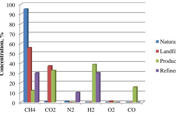
Many energy systems today involving internal combustion engines, turbines or fuel cells generate heat or electricity from natural gas. The natural gas mixture is primarily composed of C1-C4 hydrocarbons. This composition varies depending on the geographic location, time of year and other factors such as type of transportation. Due to the recent demand for natural gas, alternative methods are being utilized to produce “opportunity fuels”. Some examples of opportunity fuels are landfill gas, syngas and refinery gas. These opportunity fuels can be pipelined to utility companies, sold to nearby businesses for use in boilers, or used for onsite generation of electricity [1]. Fig. 1.1 shows typical compositions of natural gas and opportunity fuel blends. The compositions of different opportunity fuels and natural gas blends can vary quite dramatically depending on the type of fuel and production process. For example, the mole fraction of methane can be as high as 95 % in natural gas, but as low as 10 % in producer gas. The variable concentration of components in opportunity fuels results in a wide range of heating values.
2 An additional opportunity fuel of interest, producer gas, is formed by the gasification of organic material at relatively low temperatures (700 to 1000 °C). Gasification is defined as the partial oxidation of fuel at a desired temperature to produce volatile compounds (CO, H2,
CO2 and CH4) and char. The composition of gases produced depends on parameters such as
the reactor type, temperature, and the chemical characteristics of the fuel. The major products formed by the gasification reaction are carbon monoxide, hydrogen, carbon monoxide and a range of hydrocarbons with nitrogen [3].
Fig. 1.1 Typical concentration of opportunity fuels.
1.2 Conventional methods for hydrocarbon fuel mixture analysis
The composition and heating value measurement of gaseous mixtures is an important tool for any process application. For example, many gas suppliers are focused on the quality and content of the fuel which arrive at boilers, power plants and turbines. Considering the
0 10 20 30 40 50 60 70 80 90 100
CH4 CO2 N2 H2 O2 CO
3 variability in natural gas and opportunity fuel sources, it is necessary to measure a parameter which can quantify the level of interchangeability in gas mixtures, or the Wobbe index. The Wobbe index is found by taking the high heating value of the gas and dividing by the specific gravity with respect to air. The higher a gases’ Wobbe index, the greater the heating value of the gas that will flow through an orifice in a given amount of time [4]. Many methods have been developed to achieve this goal – and with the advances in technology, gas chromatography has been shown to be the most popular and accurate measurement tool, although gas calorimetry can still be effective. These methods are explained below.
1.2.1 Calorimetry
4 An indirect method of calorimetry is generally used for the measurement of natural gas heating values. In this method, a continuous gas sample is mixed with dry air at a specified air-fuel ratio, and oxidized in a combustion furnace at a set temperature. The oxygen concentration of the combusted sample is then measured and the residual oxygen can be correlated to the Wobbe Index (measure of interchangeability) of the gas [6,7].
1.2.2 Gas chromatography
The pricing of natural gas or alternative fuels is based on the heating value of the gas, which is generally determined by gas calorimetry or gas chromatography [8]. If the composition is an important parameter to measure, gas calorimetry is not helpful, as it is limited to measuring the heating value of a gas mixture. Thus, for the measurement of fuels such as natural gas or opportunity fuels, gas chromatography is the method of choice due to its ability to measure composition, as well as its excellent selectivity, increased sensitivity and expansive dynamic concentration range [9].
5 Fig. 1.2 Diagram of a gas chromatograph [10].
Gas chromatography (GC) has become the standard in measurement of composition and heating value for gaseous mixtures, but there are certainly drawbacks to this method:
Response times can be > 5 minutes; thus, not allowing real time measurements
Gas chromatographs are expensive; generally quoted at more than $20,000
Skilled operators are required to calibrate the GC, properly inject samples, and analyze chromatograph data.
Gas chromatographs must be properly maintained frequently.
6 sufficient to warrant the price of a GC. A less expensive, faster method compared to GCs is desired to measure natural gas and opportunity fuel mixtures, which is capable of making real-time composition and heating value measurements. Locations which don’t have the volume of natural gas and opportunity fuel blends to warrant the price of a GC are the target of this alternative method.
1.3 Potential alternative methods 1.3.1 Dispersive NIR spectroscopy
Applications of NIR spectroscopy were reported as early as the 1950s, but the analysis was limited to the agricultural industry at that point in time. Only since the development of improved electronic and optical components, as well as computers for data processing, has NIR spectroscopy expanded to an increasing number of fields [11] [12]. Despite its lack of specific spectral information when compared to other absorption measurement techniques, such as mid-infrared and Raman spectroscopy, NIR spectroscopy has become one of the most popular process-monitoring techniques [13].
7 heat content of opportunity fuels is generally from hydrocarbons [14]. There are three distinct absorption bands for aliphatic hydrocarbons in the near infrared region: first set of combination bands at 2000-2400 nm, first overtone at 1600-1800 nm, and second overtone at 1000-1200 nm [15]. Also of importance is CO2, which has a distinct absorption band at 2000
nm.
In order to measure these vibrational absorptions, NIR spectroscopy requires a light source to emit near infrared radiation, a sample cell to hold the gas, and a NIR spectrometer to measure the light intensity. Because overtones and combination bands are used for NIR analysis, the intensity of absorbance decreases, and thus the layer of absorbing gas (path length) must be enlarged to provide relevant spectral data [16].
1.3.2 Fourier transform infrared (FTIR) spectroscopy
8 Fig. 1.3 Optical diagram of the Michelson interferometer [17].
Light is emitted from the infrared source and reflected off the collimating mirror to make the rays parallel. The light is then separated at the beamsplitter, with a portion of the light reflected onto the moving mirror and the remaining light transmitted through to the fixed mirror. Once the beams reflect from the mirrors, they are recombined into a single beam before interacting with the sample and being collected by the detector. The optical path difference, δ, is the difference in distance travelled by the two beams and becomes an important parameter when analyzing interferograms, or interference patterns.
9 The interferogram provides a plot of light intensity versus optical path difference. A Fourier transform can then be applied to the interferogram to result in a spectrum in the frequency domain, as shown in Fig. 1.4. For a better understanding of the mathematics behind Fourier transforms, the reader is encouraged to refer to [18].
Fig. 1.4 Fourier transform applied to monochromatic radiation [17].
1.4 A literature review of NIR spectroscopy analysis 1.4.1 Quantum mechanical model
10 1. Electrons of an atom can only occupy certain discrete quantized states or orbits.
These states have different energies and the lowest energy state is referred to as the ground state.
2. When an electron transitions from one state to another, it can do so by emitting or absorbing radiation at a frequency. The frequency, ν is given by Eqn. 1.1.
1.1
where ΔE is the energy difference between the two quantized states and is Planck’s constant.
In other words, electromagnetic radiation is not emitted while an electron moves in its orbit, but only when the electron is moved from one quantum level to another. This process is called a quantum jump and is shown in Fig. 1.5 [16].
11 The number of vibrational modes for a molecule depends on the linearity and number of atoms. For a molecule containing N atoms, there are 3N-6 vibrational modes; however, for linear molecules there are 3N-5 vibrational modes [19]. Generally, the calculation of vibrational frequencies becomes difficult as the chemical structure adds complexity (polyatomic, non-linear, etc.), so a simple diatomic model (Fig. 1.6) will be analyzed first. The simple oscillator model for a diatomic molecule results in a vibrating frequency, ν:
√ 1.2
where µ is the reduced mass given by µ=mM/(m+M) and k is the force (spring) constant of the bond.
Fig. 1.6 Diatomic oscillator model.
12 Fig. 1.7 Example of (a) symmetric stretching, (b) wagging, and (c) scissoring vibrational
absorption modes.
However, to predict overtone and combination bands, normal mode theory cannot be applied, as bonds are not true harmonic oscillators [15]. As previously stated, the vibrational energy in atoms is quantized and therefore jumps from one state to another. After considering the quantized energy levels, the modified vibrational energy Evib for any molecule is given by
( ) 1.3
where is the vibrational quantum number (only integer values).
If the vibrational motion was simple oscillations, the changes in vibrational quantum number would be limited to Δν1=1, Δν2=1, and Δν3=1. Thus, only the fundamental vibrational modes
13 have overtones (Δνi>1) and combination bands (ΣΔνi>1). This causes the vibrational energy
equation to become much more complex than Eqn. 1.3 [12].
1.4.2 Beer’s law
The relationship that exists between the concentration of a single substance and the spectral absorbance is quantified by Beer’s law. If I0 is the reference spectral intensity and I is the
spectral intensity remaining after passing through the sample, the absorbance is defined as
( ) ( ( )
( )) ( ) 1.4
where σ is the absorption cross section, l is the optical path length and N is the number density of the gas molecules.
With the sample path length and absorption cross section known, the number density N of gas molecules can be calculated. An extension of Beer’s law may be applied to a mixture of gases, assuming no chemical interaction between the components:
∑
1.5
In Eqn. 1.5 Aj represents the mixture absorbance at the jth wavelength where . Ni is the
number density of the ith mixture components and σij is the absorption cross section of the ith
14 the known mixtures are correlated to their compositions using multivariate regression models. This developed model can then predict future unknown compositions.
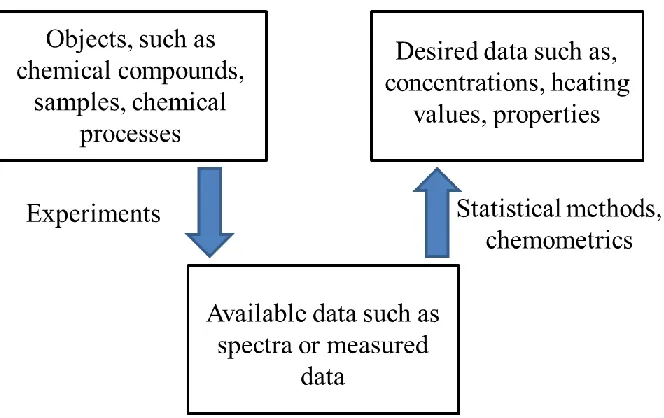
1.4.3 Multivariate methods
15 Fig. 1.8 Using chemometrics to determine difficult to measure data.
16
1.6
The columns of T represent a small set of latent variables responsible for the variation in both
X and y. Different criteria are used for the computation of the scores matrix, T, in the estimation of model parameters. P and q are referred to as loadings and give a description of how the variables in T relate to the original data in X and y. The residuals are E and f, and represent the noise or irrelevant variability in X and y, respectively.
The computation of the scores matrix T is the only difference in PLS and PCR methods, and will be discussed later. The rest of the computations are identical - loadings in P and q are estimated by regressing X and y onto T, and residuals E and f are found by subtracting TPt
and Tq from X and y, respectively. Let ̂ represent the regression vector, which is a combination of the previously computed model parameters. A prediction equation (Eqn. 1.7) can be formed to estimate the concentrations of a set of validation samples [22].
̂ ̂ ̂ ̅ ̂ 1.7
Generally the X data is mean centered before computing regression parameters, resulting in
̂ being equal to the mean centered outputs ̅. For a more detailed explanation of PCR and PLS, the reader is referred to [23], [24], and [25].
1.4.3.1 Principal components regression
17 the multicollinearity problem by creating regressor variables which are linear combinations of the original measured x-variables. PCR decomposes a mean centered data matrix ̅ into scores T and loadings P. The PCR scores have a powerful mathematical property. Because the scores are usually centered, the orthogonality between any two score vectors means the two vectors are uncorrelated [21].
The data matrix ̅ is decomposed into scores and loadings as shown in Eqn. 1.6. The covariance matrix Σ (j x j) or correlation matrix R (j x j) of ̅ is then computed. If (Λ1, e1),
(Λ2, e2)…, (Λj, ej) are the eigenvalue – eigenvector pairs of Σ, where , then
the ith principal component is given by ̅, for i = 1, 2,…., j.
The loadings matrix P is formed by taking the columns of ∑ and rearranging to the desired number of principal components. The columns are rearranged in order of importance, i.e. the first column’s eigenvalue is the largest (explains the most variance). After computing P, the scores matrix T can be calculated by regressing the mean centered ̅ onto P. The mathematical formulation of these parameters is shown in Eqn. 1.8, as well as the OLS regression calculation of the loadings matrix q.
[ ]
̅ 1.8
( )
18
̂ ̂ ̂ 1.9
The predicted property ̂ can now be calculated using Eqn. 1.7. A sample PCR model developed in MATLAB is given in Appendix A2.
1.4.3.2 Partial least squares
Partial least-squares regression (PLS) was developed in 1975 by Herman Wold, originally designed to treat chains of matrices and applications in econometrics. Herman’s son, Svante, among others, introduced the application of PLS to chemometrics. Since, PLS is considered the most widely used method in chemometrics for the calibration of multivariate data.
While PCR uses principal component scores, PLS takes components that are related to y. The PLS model uses a latent variable approach; the model tries to find a multidimensional direction in X space that explains the maximum variance in y using an iterative approach. PLS regression was developed to avoid the problem in PCR of deciding which components to use in regression.
The direction of the first PLS component is denoted by ̂ and is called the first loading weight vector. The scores ̂ , loading vector ̂ , and regression coefficient ̂ are calculated as follows. To compute the subsequent scores, loading vectors and regression coefficients the iteration starts over using X0.
19
̂ ( ) ̂
̂ ( ) ̂ 1.10
̂ ̂
̂ ̂
When the parameters are calculated for the desired number of components, the regression coefficient vector ̂ can be computed as in Eqn. 1.11.
̂ ̂( ̂ ̂) ̂ 1.11
The regression method as described here can be extended to handle several y-variables simultaneously. This PLS2 method is very similar to PLS, but the main modification is that one needs to optimize the covariance between both X and y [22].
The most commonly used algorithms for partial least squares analysis are non-linear iterative partial least squares (NIPALS) and SIMPLS. For a more in depth look at NIPALS and SIMPLS, the reader is encouraged to refer to [26] and [27], respectively. The PLSREGRESS pre-loaded MATLAB function uses the SIMPLS algorithm and is used for PLS computations in this thesis.
1.5 Thesis objectives
The results of this thesis are separated into three sections. First, experimental testing confirmed the enhanced CO2 detection capabilities using a thermoelectrically cooled
20 a non-dispersive spectral method consisting of a MEMS-FTIR was able to accurately predict opportunity fuel blends.
Chapter 1 included the background and introduction of the thesis, covering conventional methods of opportunity fuel composition and heating value measurement, along with a summary of the proposed NIR spectroscopy method. A detailed review of NIR spectroscopy was also included – Beer’s Law, multivariate regression methods, and the theory behind vibrational spectroscopy has been described. Chapter 2 describes the experimental materials and methods used in this research. Chapter 3 highlights the selection of experimental equipment as well as the accuracy of measurements, with an emphasis on uncertainty in composition prediction. Chapter 4 includes the results and discussion for the first main research topic: CO2 detection with a thermoelectrically cooled spectrometer. Chapter 5
21
2 EXPERIMENTAL APPROACH
2.1 Optical setup
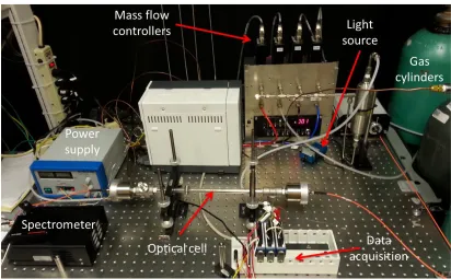
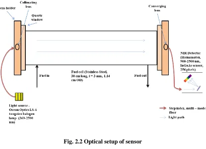
In order to experimentally measure the absorption spectra of a gaseous mixture, the hardware required is a light source, collimating and converging lens, spectrometer, and fuel cell to hold the sample, as shown in Fig. 2.1. While the fuel cell is free of absorbing species, a background and reference is captured by the spectrometer, with the light source off and on, respectively. Then a sample is placed in the fuel cell, and the spectra is collected by the spectrometer. The spectrometer normally uses a diffraction grating to separate the light into the respective wavelengths. Four mass flow controllers (MFC) are used to maintain a specified flow rate for each respective gas.
23 Fig. 2.2 Optical setup of sensor
2.2 Flow control
The fuel mixtures are prepared using four mass flow controllers (MKS 1179A). The mass flow controllers (MFC) are calibrated with N2 to full flows of 100, 1000 and 5000 standard
cubic cm per minute (SCCM). A gas correction factor is calculated for gases other than N2.
Generally, a total flow rate of 1000 SCCM is used, although the total flow rate is independent of the absorption spectra. After the individual gases exit from their MFCs, the mixing chamber creates a homogeneous mixture to pass through the sample cell for analysis.
24 channel on the power supply/readout front panel by adjusting the set point’s ten turn potentiometer. A digital panel meter displays the flow rate of any single channel of a MFC. The power supply/readout can also be controlled remotely by interfacing the P6 connector with a National Instruments (NI) data acquisition module. A detailed diagram of the pin assignments for the P6 connector is shown in Fig. 2.3.
Remote flow control is achieved by using analog output module NI9217, analog input module NI 9201 and digital output module NI 9474. A digital Boolean (on/off) signal controls the analog output module. A voltage signal, biased from 0-5 V, is then relayed by the NI 9263 module to the MFC with 5 V corresponding to full flow. Concurrently, a biased 0-5 V signal is received by the NI 9201 module to determine the actual flow rate.
25 2.3 Data acquisition system
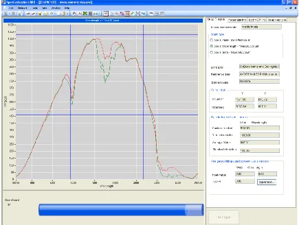
26 Fig. 2.4 Hamamatsu SpecEvaluation GUI
2.4 Experimental procedures
27 The Hamamatsu C1118GA spectrometer is connected by USB to the computer, and the previously stated GUI displays and stores spectral data captured by the photo detector. Two important parameters to set before calibration are exposure time and number of samples to average. The intensity measured by the detector array is proportional to the exposure time. The exposure time should be selected as to maximize the signal without saturating the detector. Increasing the exposure time decreases the signal-to-noise ratio, at the expense of computation time. Number of samples to average allows the user to average a selected number of samples, instead of using repeating data. The signal-to-noise ratio increases as the square root of number of samples averaged.
The detector array has a background signal even when no light is incident, called the dark current or simply background. Therefore, after allowing the spectrometer to warm up and with the light source off, a dark current should be measured. This dark current is subtracted from all future measurements as it is just a measure of residual electric signal within the detector. A non-absorbing NIR gas, such as N2, is then used to purge the sample cell for
10-15 minutes to remove any residual absorbing gases. After allowing the light source to warm up, a reference intensity is captured and is representative of the wavelength characteristics of the light source. For clarity, the background and reference does not need to be recalculated for every sample. The desired flow rates are input in the LabVIEW program and the
29
3 EQUIPMENT SELECTION AND ACCURACY OF MEASUREMENTS
3.1 Selection of spectral range
Referring back to Section 1.1, it is evident that to quantify opportunity fuel mixtures, the detection of CH4, CO2 and C3H8 is of importance. Diatomic atoms such as N2, H2 and O2 are
NIR inactive so these molecules will not be further investigated.
The HITRAN (high resolution transmission) molecular absorption database is a compilation of parameters spectroscopists use to predict and simulate the emission and transmission of a wide range of compounds. The database is developed and maintained at the Harvard-Smithsonian Center for Astrophysics in Cambridge. Before selecting a wavelength range and resolution for a spectrometer, HITRAN data was used to research the previously mentioned gases.
30 Fig. 3.1 HITRAN high resolution spectra of CO2.
Diffraction type spectrometers have a low resolution profile, depending on the slit size and other mechanical properties. Thus, it is necessary to convolute the high resolution HITRAN data to a lower resolution to match the diffraction grated spectrometer’s profile.
3.1.1 Spectral convolution
Diffraction type spectrometers are limited by the slit size and the size of the photodetector within. To estimate the spectra likely to be seen by the spectrometer, a convolution filter needs to be applied to the high resolution HITRAN data as in Eqn. 3.1.
1500 1600 1700 1800 1900 2000 2100 2200 2300 2400 2500 -0.5
0 0.5 1 1.5 2 2.5 3
Wavelength, nm
A
bs
or
ba
nc
31
( )( ) ∫ ( ) ( )
3.1
( ) {
The high resolution spectra from HITRAN is represented by f (λ) and g (λ – τ) is the unity square wave which is shifted by a τ step. Because the wavelength spacing in the spectrometer used is non-uniform, the dτ value changes between each iteration. The convolution code developed in MATLAB is available in Appendix A2. Refer to Fig. 3.2 for the result of a convoluted CO2 spectra from Fig. 3.1.
Fig. 3.2 Convoluted spectra of CO2
15000 1600 1700 1800 1900 2000 2100 2200 2300 2400 2500
0.05 0.1 0.15 0.2 0.25 0.3 0.35 0.4
Wavelength, nm
A
bs
or
ba
nc
e
32 3.2 Spectrometer selection
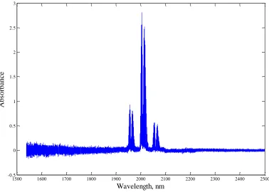
The HITRAN database was used to estimate the absorption bands of the primary components of opportunity fuels. For example, the spectra of CO2, CH4, C3H8 and H2O at 52 °C and 100
% RH is shown in Fig. 3.3. Previous spectroscopic methods have had poor CO2 detection
capability due to the limited range of common NIR spectrometers (1700 nm maximum), so it is desirable to find a long wavelength spectrometer (1200 – 2200 nm) to include the major CO2 absorption band at 2000 nm. A Hamamatsu C11118GA thermoelectrically cooled
spectrometer offers a spectral response from 900-2550 nm and is selected for this research application.
Fig. 3.3 Measured spectra of carbon dioxide, methane, propane and nitrogen humidified with water vapor at 52°C and 100 % RH.
33 3.3 Spectral uncertainty
3.3.1 Signal-to-noise ratio
Signal-to-noise ratio (SNR) is a measure used in spectroscopic systems to compare the level of signal to background noise. Many items of interest, such as sensitivity, repeatability, and signal accuracy depend on the SNR.
The SNR changes for different wavelengths due to the detector, because of the varied intensity incident on the photo-detector. A reference intensity is measured repeatedly with no absorbing gases in the path length before starting SNR calculations. An example of this reference intensity (which includes Teflon filter absorption) is shown in Fig. 3.4.
34 The noise n(λ) is calculated by taking the root mean square of the reference intensity I(λ) measured N times as shown in Eqn. 3.2. The noise spectra should be a horizontal line of zero, ideally. However, noise appears in most systems and must be calculated; an example of a noise spectra is shown in
( ) √∑( ( ) ( )) 3.2
Fig. 3.5 Noise spectra
800 1000 1200 1400 1600 1800 2000 2200 2400 2600
0.8 1 1.2 1.4 1.6 1.8 2 2.2 2.4 2.6
Wavelength, nm
N
oi
se
,
A
/D
c
ount
35 After the noise spectrum is calculated, the SNR can be found by taking the ratio of the signal and the noise, as shown in Eqn. 3.3. With increasing SNR, the repeatability, accuracy, and detection increases for the system.
( ) ( )
( ) 3.3
An example of the SNR for a long wavelength spectrometer is shown in Fig. 3.6.
Fig. 3.6 Signal-to-noise ratio (SNR)
36 3.3.2 Selectivity and limit of detection
In classical multivariate calibration, such as principal components analysis, figures of merit can easily be calculated once the net analyte signal (NAS) is derived. To find selectivity, one must first take the principal components obtained from the spectra of interfering components and project on to the spectrum of the component to be quantified. The projected spectrum is then subtracted from the pure absorption spectrum of the component of interest. The remaining spectrum is now considered the NAS specific to the target component and represents the portion of the spectrum orthogonal to the spectra of other components. Lorber [29] defines selectivity as in Eqn. 3.4.
( )
3.4
‖ ‖ ‖ ‖
Where I is the identity matrix, v is the matrix of eigenvectors, a is the analyte absorption spectrum, a* is the NAS, SEL is the selectivity and ‖ ‖ represents the Euclidean norm. SEL
has a bounded magnitude from 0 to 1, with 0 indicating no selectivity and 1 representing a fully selective signal. Table 1 shows the selectivity values calculated using Eqn. 3.4.
Table 1. Selectivity and limits of detection using 6 principal components.
SEL LOD, %
CH4 0.113 0.288
CO2 0.282 0.164
37 3.4 Mass flow controller uncertainty
The uncertainty in mixture compositions is largely dependent on mass flow controller (MFC) accuracies. Four MFCs control individual pure gases with a 1% full scale accuracy. Say mi
is the desired flow rate in SCCM for the ith component where i=1 to n and dmi represents the
error in mass flow rate of the ith component. The total desired flow rate becomes m and the error in mole fraction dXi for the ith component can be calculated as below.
∑ ∑ 3.5 ∑ ∑ ∑
Considering n mass flow controllers, Eqn. 3.5 results in the following.
( ) 3.6
( ) ( ) ( ) ( ) ( )
( ) ( )
3.7
Take a four component mixture of 10 % C3H8, 15 % CO2, 60 % CH4, and 15 % N2 at a total
38 and 5000 SCCM full flow, respectively. Using Eqn. 3.5 and 3.7, the uncertainties in the individual flow rates and uncertainties in mole fractions are given in Table 2.
To compute a composite uncertainty, the uncertainties from the mass flow controller and from the limits of detection are combined. If dX is the composite error, the contributions from mass flow controller uncertainty (dXmfc) and from the net analyte signal method (dXnas)
are equated by √ .
Table 2. Uncertainty in flow rate and composition for each mixture component.
dm,
SCCM
composite
dX, %
C3H8 5 0.85
CO2 10 1.37
39
4 ENHANCED CO2 DETECTION WITH A THERMOELECTRICALLY COOLED
SPECTROMETER TO PROVIDE BROADER SPECTRAL RANGE 4.1 Experimental validation
40 Table 3. Laboratory calibration and validation mixtures.
% C3H8 % CO2 % CH4 % N2
HV
(MJ/m3)
ca li b ra ti o n
10 0 90 0 43.50
10 5 80 5 39.72
10 10 70 10 35.95
10 15 60 15 32.18
10 20 50 20 28.40
5 25 40 30 19.86
5 30 30 35 16.09
5 35 20 40 12.31
5 40 10 45 8.54
5 45 0 50 4.77
5 50 0 45 4.77
v a li d a ti o n
10 45 0 45 9.53
10 40 10 40 13.31
10 35 20 35 17.08
10 30 30 30 20.85
10 25 40 25 24.63
5 20 50 25 23.64
5 15 60 20 27.41
5 10 70 15 31.18
41 Fig. 4.1 Resulting spectra of 11 calibration mixtures.
4.2 Results and discussion
The calibration composition and heating values are saved in a matrix and PCR/PLS methods are applied to the absorption data. To evaluate the accuracy of the model, a root mean square error of prediction (RMSEP) is calculated for each species. If yset and ypred are the set and
predicted properties, and n is the number of validation samples to be tested, the RMSEP is defined as follows:
√∑( ) 4.1
1200 1300 1400 1500 1600 1700 1800 1900 2000 2100 2200
42 The PLS and PCR models have very similar results, so only the PCR results will be
discussed. Using Eqn. 4.1 the RMSEP for 6 principal components with PCR is 0.25 %, 0.41 %, 0.94 %, 1.06 % and 0.21 MJ/m3 for propane, carbon dioxide, methane, nitrogen and heating value, respectively. The estimated concentrations of carbon dioxide have higher prediction accuracy compared to methane and propane, which is likely due to the distinct carbon dioxide absorption band from 1950-2100 nm.
43 Increasing the number of principal components used allows for more spectral variance to be explained (Fig. 4.3) and in turn reduces the RMSEP.
Fig. 4.3 Variance explained by each PLS component.
1 2 3 4 5 6
98.5 99 99.5 100
Number of PLS components
P
e
rc
e
nt
V
a
ri
a
nc
e
E
xpl
a
ine
d
in
44
5 WATER VAPOR QUANTIFICATION WITH A THERMOELECTRICALLY
COOLED SPECTROMETER 5.1 Background
Water vapor is commonly absorbed in natural gas mixtures, especially in landfill gas. Dehumidification systems are in place to remove the water, but there is always the potential for water to remain in these mixtures. Water vapor can be potentially very harmful and even destructive to power plant machinery if not properly removed. Because water vapor is active in the near infrared range, a direct injection system is developed to test for the recognition of water vapor in gaseous mixtures.
Synthetic line-by-line absorbance data for H2O is obtained from the HITRAN on the web
45 Fig. 5.1 Simulated spectra consisting of convoluted HITRAN data.
The H2O absorption band in the 1800-2000 nm range offers distinction from alkane and CO2
absorptions and will be sufficient for the spectral recognition of water vapor.
5.1.1 Psychrometrics
With the help of psychrometric equations, the injection rate of H2O can be varied to humidify
a gaseous mixture to a specific relative humidity. The flow rate of N2 is kept at a constant
rate of 1 LPM and the temperature of the sample cell is stabilized. First, the partial pressure of water vapor is defined in Eqn. 5.1
5.1
13000 1400 1500 1600 1700 1800 1900 2000 2100
46 Where is the partial pressure of water vapor given in kPa, is the saturation
pressure of water vapor at temperature T, and is the relative humidity, representing the ratio of water vapor to the water vapor present if saturated at T. is found by using the Goff-Gratch equation, and is dependent on temperature [30].
5.2
The partial pressure of N2 is found by subtracting the partial pressure of H2O from
atmospheric pressure.
5.3
Where and represent the molar mass in g/mol of H2O and N2, respectively, and
is the humidity ratio of the mixture in g water vapor/g N2.
An ideal gas at standard conditions (25º C and 1 atm) has a molar volume of 24 L/mol. Given the volume flow rate, the mass flow rate of N2 can be calculated as shown in Eqn. 5.4.
̇ ̇
5.4
where ̇ is the mass flow rate of N2 in g vapor/min, and ̇ is the volume flow rate of N2
in liters/min. After finding the humidity ratio and mass flow rate of N2, the required rate of
47
̇ ̇ 5.5
5.2 Experimental approach
Fig. 5.2 shows the experimental setup for the water vapor quantification experiment which is similar to the existing setup, with the inclusion of a few new components. A direct injection syringe pump is inserted to add water at a set rate to the gaseous mixture, and a heating system (400 W and 60 °C maximum) is designed and implemented for sample cell heating.
48 5.2.1 Experimental equipment and setup
Deionized (DI) water is directly injected to an evaporation chamber, where the water humidifies the gas mixture. The output from the evaporation chamber travels through heated piping to the sample cell. As shown in Fig. 5.2, the mixture coils around the sample cell inside a heating chamber to insure the temperature is stabilized. Spectral measurements are made as before and the mixture finally goes to exhaust. A complete schematic of the experimental setup is shown in Fig. 5.3.
49 A 60 ml syringe (BD Luer-Lok) is filled with DI water and housed on a Cole-Parmer 115 V/0.1 A step motor. Depending on the diameter of the syringe used, the step motor can be adjusted to control the injection rate of water. A Variac (0-135 V) autotransformer is used to control the heating of flexible heating strips applied at the evaporation chamber and sample cell heating chamber. The 5 cm diameter stainless steel evaporation chamber takes N2 and
H2O and heats to evaporation – the chamber is filled with silicone beads to provide uniform
heating. A temperature controller (Omega CN 77532-A2) uses PID control to heat two auxiliary heating strips wired in series to a desired temperature (set point). A detailed diagram of the pin positions for the Omega temperature controller is shown in Fig. 5.4. The auxiliary heating strips are included to prevent the vapor from condensing between the evaporation chamber and the sample cell. The sample cell is enclosed in the cylindrical heating chamber and the central axis is uniformly heated due to free convection.
50 The temperature of the evaporation chamber, humidity sensor exit and cylindrical enclosure central axis are measured using type K thermocouples connected to NI 9211. The temperature and humidity of the sample are measured with a humidity sensor (Omega, HX93AC) – the humidity sensor is measured in cross flow with the incoming mixture to avoid accumulation (Fig. 5.5). The measurements made by the sensor are relayed to the computer as an analog current signal (4-20 mA) using a NI 9203 analog input module.
Fig. 5.5 Humidity sensor orientation
5.2.2 Experimental conditions
To test for the composition and heating value of a mixture containing CH4, C3H8, and H2O,
51 Table 4. Experimental parameters
T, fuel cell (°C) 49 Exposure (µs) 500 # of samples to average 20
The composition matrix was formed using the mass fraction % of the components, as well as the heating value, and can be found in Table 5. The total flow rates used for all mixtures remained between 1000-1020 SCCM.
Table 5. Experimental mixture composition and heating values.
% C3H8 % H2O % CH4
HV (MJ/m3)
tr
ai
n
0.00 3.65 96.35 39.84 4.99 3.47 91.54 37.85 4.88 5.65 89.47 39.15 0.00 5.94 94.06 41.16 0.00 9.17 90.83 43.02 4.72 8.74 86.54 40.99
te
st
52 The injection rate of H2O was increased from 1.5 mL/hr, 2.5 mL/hr to 4 mL/hr every two
samples for the 6 training mixtures. To illustrate the spectral variation this increase in H2O
caused, Fig. 5.6 shows the six training mixture spectra.
Fig. 5.6 Training mixture spectra
5.2.3 Results and discussion
The calibration composition and heating values were saved in a matrix and PCR/PLS methods were applied to the absorption data. Using Eqn. 4.1 the RMSEP using 5 principal components with PCR was 0.34 %, 0.43 %, 0.59 % and 0.21 MJ/m3 for propane, water vapor, methane, and heating value, respectively. The RMSEP is essentially an average of the four validation tests, where the individual error obtained from each test is shown in Table 6.
1200 1300 1400 1500 1600 1700 1800 1900 2000
0 0.05 0.1
Wavelength,nm
A
bs
or
ba
nc
e
53 Table 6. Prediction error for individual validation mixtures (PCR with 5 components).
Error
% C3H8 % H2O % CH4 HV (MJ/m3)
Test 1 0.126 0.261 0.135 0.168
Test 2 0.151 0.328 0.479 0.037
Test 3 0.658 0.061 0.719 0.352
Test 4 0.040 0.748 0.788 0.261
Increasing the number of principal components used allows for more spectral variance to be explained and in turn reduces the RMSEP. This is illustrated in Fig. 5.7. The predicted values using PLS were very similar to those using PCR, therefore the PLS results are omitted.
Fig. 5.7 RMSEP dependence on number of components.
0.00 0.50 1.00 1.50 2.00 2.50
2 comp 3 comp 5 comp
54 Fig. 5.8 illustrates the predictions made of individual components and the relationship to the ideal zero error situation.
55 Water vapor is proven to be accurately detected by the long wavelength Hamamatsu
spectrometer, and the principal components calibration model gives reasonable composition prediction results. The distinct H2O absorption band from 1800-2000 nm allows for accurate
56
6 A NON-DISPERSIVE SPECTRAL METHOD TO ACCURATELY PREDICT
OPPORTUNITY FUEL BLENDS: MEMS-FTIR
The world’s first MEMS-fabricated ultra-small Fourier transform infrared (FTIR) engine was developed by Hamamatsu in 2013. The application of this instrument to the detection of opportunity fuel mixtures will be discussed below. Also, the results of the FTIR will be compared to those of the diffraction grating type spectrometer.
6.1 Experimental methods
The experimental setup is very similar to that from the CO2 detection using a Hamamatsu
C11118GA spectrometer, with the exception of a new high powered light source, new fiber cable, and different spectral software.
The Ocean Optics LS-1-LL tungsten halogen lamp light source is replaced by a high powered Thorlabs OSL1 (150 W) light source coupled with an OSL2BIR (Enhanced IR, 3200 K) bulb. An OSL1-SMA fiber adapter is fit to the light source to allow for an SMA-type fiber connection. The FTIR has an FC type connector, so the SMA-SMA fiber cable is replaced with a SMA-FC.
57 the cost of computation time. 6000 ms has been found to be a favorable exposure time for the experimental setup.
Fig. 6.1 Si-Ware FTIR spectral software GUI
6.2 Results and discussion
The four component test from Section 5.1 is duplicated with 11 calibration and 9 validation mixtures prepared as in Table 3. The data from Si-Ware is truncated to include only 1600-2100 nm wavelengths – this eliminates the noisy data (1200-1600 nm) from the PCR and PLS model. The RMSEP of the validation mixtures is shown in Table 7. When using 6 components and the PCR model, C3H8, CO2, CH4, N2 have an error of 1.2%, 1.3 %, 3.8 %
58 Table 7. Prediction error using principal components regression (PCR) and partial least
squares (PLS).
RMSEP
2 comp 3 comp 6 comp
PCR
% C3H8 3.078 3.065 1.187
% CO2 5.519 4.765 1.302
% CH4 11.793 8.655 3.844
% N2 5.128 2.544 2.597
HV (MJ/m3) 2.616 0.566 0.532
PLS
% C3H8 3.601 2.792 0.886
% CO2 4.920 3.860 1.983
% CH4 10.437 7.005 3.311
% N2 2.456 2.455 4.360
HV (MJ/m3) 0.824 0.523 1.022
59 Fig. 6.2 Comparison of CH4 prediction with 6 components using (a) MEMS-FTIR and
(b) dispersive grated NIR spectrometer.
60 Fig. 6.4 Comparison of C3H8 Prediction with 6 components using (a) MEMS-FTIR and
61 CONCLUSIONS
A diffraction grating based NIR spectroscopy method and multivariate regression models have been developed to quantify C1-C4 alkanes, water vapor and specifically CO2
composition in natural gas and opportunity fuel mixtures. The primary challenge in the existing optical sensor setup was CO2 detection in the NIR range. A thermoelectrically
cooled spectrometer provides an extended wavelength range to include a distinct CO2
absorption band. It is proven that the long wavelength spectrometer, with multivariate methods, can estimate component concentrations to a level comparable (~1 %) to gas chromatographs (GC).
An experimental setup, consisting of mass flow control system, data acquisition and optical components have been outlined. Multivariate prediction methods, such as PLS and PCR, process the spectral data to predict component concentrations. The benefits of the system are enhanced CO2 detection, increased water vapor detection and greater accuracy in prediction.
62 The experimental setup is modified for the water vapor quantification test. Water is directly injected, before being heated and humidified into the gaseous mixture. Temperature is controlled along the gas line, and the previously stated multivariate methods are used to make predictions of component mass fractions. The increased wavelength range makes water vapor easier to detect with the inclusion of a distinct absorption band from 1800-2000 nm.
A non-dispersive alternative method is investigated, where a MEMS Fourier transform infrared (FTIR) spectrometer replaces the dispersive long wavelength spectrometer. The FTIR is smaller and cheaper than most dispersive spectrometers, and thus would help this sensor to become commercialized. Composition predictions are compared to those from the long wavelength spectrometer and it is discovered that the FTIR is slower (~90 s response) and less accurate (4 % RMSEP) than the previous method. Additional studies are needed to correctly implement the FTIR within the current gas detection method.
63 mass flow controller having a full flow of 5000 SCCM, as opposed to the 1000 SCCM for CO2.
The increased accuracy in CO2 prediction, as well as the detection of water vapor in the
larger wavelength range show that the optical gas sensor is well suited for industrial process control purposes. The study is applicable to mostly landfill gas mixtures, where CH4 is the
main component, but can also apply to other opportunity fuels (given auxiliary sensors to detect gases such as H2, CO and O2). The water vapor detection capability would allow the
64 FUTURE WORK
65 REFERENCES
1. Goossens, MA. "Landfill Gas Power Plants." Renewable Energy 9.1 (1996): 1015-8.
2. Eklund, Bart, et al. "Characterization of Landfill Gas Composition at the Fresh Kills Municipal Solid-Waste Landfill." Environmental science & technology 32.15 (1998): 2233-7.
3. Sadaka, Samy. "Gasification, Producer Gas and Syngas." (2009).
4. Emerson Process Management. The Wobbe Index and Natural Gas Interchangeability., 2007.
5. Kolesov, VP. "Bomb Combustion of Gaseous Compounds in Oxygen." Experimental Chemical Thermodynamics 1 (1979): 1-16.
6. Ulbig, Peter, and Detlev Hoburg. "Determination of the Calorific Value of Natural Gas by Different Methods." Thermochimica Acta 382.1–2 (2002): 27-35.
7. Foundos, P., G. Liptak, and D. Lewko. "8.8 Calorimeters." (2003).
66 9. Klemp, Mark, Anita Peters, and Richard Sacks. "High-Speed GC Analysis of VOCs:
Sample Collection and Inlet Systems. 1." Environmental science & technology 28.8 (1994): 369A-76A.
10. McNair, Harold M., and James M. Miller. Basic Gas Chromatography. John Wiley & Sons, 2011.
11. Blanco, M., and I. Villarroya. "NIR Spectroscopy: A Rapid-Response Analytical Tool."
TrAC Trends in Analytical Chemistry 21.4 (2002): 240-50.
12. Siesler, Heinz W., et al. Near-Infrared Spectroscopy: Principles, Instruments, Applications. Wiley. com, 2008.
13. Ding, Qing, Gary W. Small, and Mark A. Arnold. "Evaluation of Nonlinear Model Building Strategies for the Determination of Glucose in Biological Matrices by Near-Infrared Spectroscopy." Analytica Chimica Acta 384.3 (1999): 333-43.
14. Sutherland, G. "BBM, Discussions Faraday Sot." (1950).
15. Workman Jr, Jerry, and Lois Weyer. Practical Guide to Interpretive Near-Infrared Spectroscopy. CRC press, 2007.
16. Herzberg, Gerhard. Spectra of Diatomic Molecules. 1 Vol. van Nostrand, 1950.
67 18. Kauppinen, Jyrki, and Jari Partanen. Fourier Transforms in Spectroscopy. Wiley Online
Library, 2001.
19. Fowles, Grant R. Introduction to Modern Optics. Courier Dover Publications, 1975.
20. Gasteiger, Johann, and Thomas Engel. Chemoinformatics: A Textbook. John Wiley & Sons, 2006.
21. Varmuza, Kurt, and Peter Filzmoser. Introduction to Multivariate Statistical Analysis in Chemometrics. CRC press, 2009.
22. Næs, Tormod, et al. A User-Friendly Guide to Multivariate Calibration and Classification. 6 Vol. NIR publications Chichester, 2002.
23. Hasegawa, Takeshi. "Principal Component Regression and Partial Least Squares Modeling." Handbook of vibrational spectroscopy (2002).
24. Ge, Zhiqiang, and Zhihuan Song. "Subspace Partial Least Squares Model for Multivariate Spectroscopic Calibration." Chemometrics and Intelligent Laboratory Systems (2013).
25. Fuller, MP, GL Ritter, and CS Draper. "Partial Least-Squares Quantitative Analysis of Infrared Spectroscopic Data. Part I: Algorithm Implementation." Applied Spectroscopy
42.2 (1988): 217-27.
26. de Jong, Sijmen. "SIMPLS: An Alternative Approach to Partial Least Squares
68 27. Geladi, Paul, and Bruce R. Kowalski. "Partial Least-Squares Regression: A Tutorial."
Analytica Chimica Acta 185 (1986): 1-17.
28. Jangale, Vilas. "Optical Gas Quality Sensor for Natural Gas and Opportunity Fuels." (2010).
29. Lorber, Avraham. "Error Propagation and Figures of Merit for Quantification by Solving Matrix Equations." Analytical Chemistry 58.6 (1986): 1167-72.
30. Goff, John A., and Serge Gratch. "Low-Pressure Properties of Water from-160 to 212 F."
70 APPENDIX A1
% This program is intended to convolute high resolution data from HITRAN % to match the spacing of the spectrometer using numerical (trapezoidal) % integration
%substance to be convoluted
specs='CH4';
%read in .mat files containing spectral data from hitran (ch4.mat) and %the spectrometer (hamma_range.mat)
load('ch4.mat')
load('hamma_range.mat')
%%
%synethic data to be convoluted
wavenum=data(:,1); abs=data(:,2);
%hammamatsu spectrometer data is named hamma_wavenum and hamma_wavelen
%getting size of matrix/arrays
[a,b]=size(abs);
[a2,b2]=size(hamma_wavelen); a3=round(a2/2)+1;
%conversion from wavenum to wavelength
wavelen=zeros(length(wavenum),1);
for i=1:length(wavenum)
wavelen(i)=10^7/wavenum(i);
end
%calculating area between adjacent cells using trapezoidal integration
area=zeros(a,1);
for i=1:a
if i == a
area(i)=area(i-1);
else
area(i)=(abs(i)+abs(i+1))/2*(wavelen(i)-wavelen(i+1));
end
end
%setting up zero arrays before loop
71
for i=1:2:a2
ar=0; cnt=0;
%using hitran data at hammamatsu intervals
while wavelen(j) > hamma_wavelen(i) ar=ar+area(j);
cnt=cnt+1;
% fprintf('%i\n',j)
j=j+1;
end
areas(num)=ar;
wavelen1(num)=(wavelen(j-cnt)+wavelen(j))/2; %convoluted wavelength
absorb(num)=ar/(wavelen(j-cnt)-wavelen(j)); %convoluted absorbance
count(num)=cnt;
% fprintf('%i\n',j)
num=num+1;
72 APPENDIX A2
%Peter Finnegan %Oct 22,2013 %
%PCR Multivariate analysis
%Program to take spectral data and make composition and HV predictions %using PCR and PLS methods
%% Importing data from Hammamatsu spectrometer
h_col=1;
N=input('Enter the number of train files you have\n');
N_t=input('\nEnter the number of test files you have\n');
NPC=input('\nHow many Principal components?\n');
h_row=24; %usually 24 .csv
for i=1:N
fileName=['train' num2str(i)];
D.(fileName)=csvread([fileName '.csv'],h_row,h_col);
end
for i=1:N_t
fileName=['test' num2str(i)];
D.(fileName)=csvread([fileName '.csv'],h_row,h_col);
end
N_H=3; %# of header lines
temp_prop = importdata('temp.txt','\t',N_H);
RH=temp_prop.data(:,6); %measured RH
%% Data manipulation
%When creating train and ref matrices, include D.train(i) up to # of train %files
wavelen = D.train1(:,1); dark = D.train1(:,2);
train = [D.train1(:,4) D.train2(:,4) D.train3(:,4) D.train4(:,4)...
D.train5(:,4) D.train6(:,4)];
ref = [D.train1(:,3) D.train2(:,3) D.train3(:,3) D.train4(:,3)...
D.train5(:,3) D.train6(:,3)];
%Enter min and mix rows to chop the ends of data
% min=1; max=256; %for full spectra
min=48; max=194; %for truncated
wavelen=wavelen(min:max); dark=dark(min:max);
73
train=train(min:max,:); ref=ref(min:max,:);
%conversion from raw a/d counts to absorbance
[a,b]=size(train); train_spec=zeros(a,b);
for i=1:a
for j=1:b
train_spec(i,j)= -log10((train(i,j)-dark(i))/(ref(i,j)-dark(i)));
if train_spec(i,j) < 0
train_spec(i,j) = 0;
end
end
end
%% PCA
N_H=1; %# of header lines
%Import composition data from simple .txt file
train_prop = importdata('train_composition.txt','\t',N_H);
X = (train_spec)'; Y = train_prop.data;
[nrow,ncol]=size(X); %nrow=#samples ncol=#wavelengths
[nrowy,ncoly]=size(Y);
%mean centering data
av=zeros(1,ncol); avy=zeros(1,ncoly);
Xbar=zeros(nrow,ncol);Ybar=zeros(nrow,ncoly);ybar=zeros(1,ncoly);
for i=1:nrow
for j=1:ncol
av(j)=mean(X(:,j));
Xbar(i,:)=X(i,:)-av; %subtracting mean
end
for k=1:ncoly
avy(k)=mean(Y(:,k));
Ybar(i,:)=Y(i,:)-avy; %subtracting mean
ybar(1,k)=mean(Y(:,k));
end
end
%% PCR parameter calcs
S=cov(Xbar); %covariance
R=corrcoef(Xbar); %correlation
[v,d]=eig(S); %e-vec and e-vals of covariance
[d order] = sort(diag(d),'descend'); %sorting diagonals
74
P=v(:,1:NPC); %loadings w/ important columns
T=Xbar*P; %scores matrix
q=(T'*T)\T'*Ybar; %loadings
%% Insert test data below
test = [D.test1(:,4) D.test2(:,4) D.test3(:,4) D.test4(:,4)]; test_ref = [D.test1(:,3) D.test2(:,3) D.test3(:,3) D.test4(:,3)];
test = test(min:max,:);
test_ref = test_ref(min:max,:);
[a,b]=size(test);
test_spectra=zeros(a,b);
%dark subtraction and Beer's law
for i=1:a
for j=1:b
test_spectra(i,j)= -log10((test(i,j)-dark(i))/(test_ref(i,j)-dark(i)));
if test_spectra(i,j) < 0
test_spectra(i,j) = 0;
end
end
end
%Mean subtraction
X1 = (test_spectra)'; [n1,c1]=size(X1);
avt=zeros(1,c1); X1bar=zeros(n1,c1);
for i=1:n1
X1bar(i,:)=X1(i,:)-av; %subtracting mean
end
T1=X1bar*P;
%% Prediction
Y1=zeros(n1,ncoly);
for i=1:n1
Y1(i,:)=ybar+T1(i,:)*q;
end
%Variance in each component calcs
N_d=length(d); var=zeros(N_d,1);
for i=1:N_d
var(i)= d(i)/sum(d);
end
%% legend
%calculating length of string for legend
l_str=zeros(nrowy,1);
75
l_str(i)=length(sprintf('%.1f C3H8, %.1f H2O, and %.1f
CH4',Y(i,1),Y(i,2),Y(i,3)));
end
sleg=char.empty(0,l_str);
for i=1:nrowy
lim=l_str(i);
sleg(i,1:lim)=sprintf('%.1f C3H8, %.1f H2O, and %.1f
CH4',Y(i,1),Y(i,2),Y(i,3));
end
%% Plotting absorbance spectrum
figure(1)
plot(wavelen,X)
grid on
% axis([800 2500 0 1])
axis([1200 2000 -.005 .15]) legend(sleg)
xlabel('Wavelength,nm')
![Fig. 1.2 Diagram of a gas chromatograph [10].](https://thumb-us.123doks.com/thumbv2/123dok_us/1408434.1173443/16.612.164.490.72.272/fig-diagram-of-a-gas-chromatograph.webp)
![Fig. 1.4 Fourier transform applied to monochromatic radiation [17].](https://thumb-us.123doks.com/thumbv2/123dok_us/1408434.1173443/20.612.133.498.213.427/fig-fourier-transform-applied-monochromatic-radiation.webp)
![Fig. 2.3 Interface connector P6 pinout for mass flow controllers [28].](https://thumb-us.123doks.com/thumbv2/123dok_us/1408434.1173443/35.612.234.396.378.569/fig-interface-connector-p-pinout-mass-flow-controllers.webp)