Electron and Photon Interactions
with Molecules
by
All Abed All El-Zein
A thesis in partial fulfilment for the
degree o f Doctor o f Philosophy
ProQuest Number: U642166
All rights reserved
INFORMATION TO ALL USERS
The quality of this reproduction is dependent upon the quality of the copy submitted. In the unlikely event that the author did not send a complete manuscript and there are missing pages, these will be noted. Also, if material had to be removed,
a note will indicate the deletion.
uest.
ProQuest U642166
Published by ProQuest LLC(2015). Copyright of the Dissertation is held by the Author. All rights reserved.
This work is protected against unauthorized copying under Title 17, United States Code. Microform Edition © ProQuest LLC.
ProQuest LLC
789 East Eisenhower Parkway P.O. Box 1346
Abstract
Electron interaction with H2O molecules (chapters 1 to 4) are studied to determine the absolute differential (DCS) and integral (ICS) cross sections for the electron impact excitation of the vibrational symmetric bending (0 1 0) and unresolved symmetric + asymmetric stretching (100+001) modes respectively. The energy o f the incident electron beam ranges from 6 to 20 eV with the scattering angle varying from 10° to 135°. The scattered electrons show significant angular structure in both the
(010) and the (100+001) DCSs due to decay from Feshbach resonances in H2O' with a
6 2 symmetry state. This observation agrees for the first time with theoretical studies, and the H2O grand total cross section (GTS) results confirm the earlier experimental findings.
Femtosecond photon interactions with xenon atoms (chapters 5 to 7) are studied by scanning a focused laser spot along the direction o f propagation and using a sub-millimetre aperture detector that exposes regions o f different laser intensities to the detector. The ion signal from different regions o f the laser focus varies as a function of intensity within the confocal volume. Fitting the ion signal to the intensity volume shell allows detailed deductions to be made of the laser molecule interactions as a function of laser intensity. This has shown ionisation suppression in high intensity short laser pulses.
All love to
my father, w ho died before the com pletion o f this work,
m y m other for her encouragem ent
m y sisters and brother for their support.
A n d
tfie eartfi repÇied ivftenI
asked:“Do you motfier hate the human kind?**
“I hCess those, with ambitions, onjoy hazardous ride.
I curse the one who does not wafk with the time
and accepts the sofid way in the fife.
Look creature struyyfe to survive
and insuft the dead, however, is farye. **
“You yuardmoney, hut knowfedye yuards you. ** Ali Bin Abi Taleb
(^)
-Acknowledgements
Prof W. H Newell, my supervisor, and Dr A. C. H. Smith, my second supervisor. Dr J. H. Sanderson, PDRA, and Dr M. J. Brunger for their guidance and advice. Prof Z). H. Davis for his support and Dr J. H, Bartley who advised me to change to physics.
Prof I. D. Willimas for his collaboration.
My colleagues in the group W. A. Bryan, T. R. J. Goodworth and P. McKenna for listening and discussion.
The staff of ASTRA Central Laser Facility at Rutherford Appleton Laboratory for their experience and instruction in the femtosecond laser system.
My family who motivated me to restart my study.
My friends for encouragement.
Contents
Page
Abstract 2
Acknowledgements 4
Contents 5
List of figures 1 1
List of tables 24
Chapter 1 - Electron Scattering Theoretical Review
261.1 Cross Section Definition 26
1.2 Basic Scattering Theory 28
1.2.1 Partial Wave Decomposition 30
1.2.2 Expansion of Full Asymptotic Solution 30
1.3 Electron-Molecule Scattering Theory 31
1.4 Methods of Theoretical Calculations 33
1.5 Analysis of Experimental Results 3 5
1. 6 Resonance Processes in Electron Scattering 36
1.7 Resonance Phase Shift 3 8
1.8 Fundamental Processes in Electron-Molecule Collisions 39
1.9 Summary 39
Chapter 2 - Electron Scattering Experimental Setup
41
2.1 Experimental Chamber 41
2.2 Magnetic Shielding 42
2.3 Vacuum System 43
2.4 The Secondary Base Plate (SBP) 46
2.5 The Mechanical Design of the Analyser 47
2.6 The Gas Line 47
2.7 The Electron Lenses 49
2.7.1 Imaging of an Electron Beam 50
2.7.2 Aberrations 52
-2.8 The Electron Spectrometer Monochromator 55
2.8.1 The Electron Source 55
2.8.1.1 Configuration of Electron Emission System 56
2.8.1.2 Electron Emission and Pencil Angle 56
2.8.2 The Electron Gun 58
2.8.3 Hemispherical Energy Monochromator 62
2.8.4 The Pre-Interaction Region Lenses 65
2.9 The Interaction Region 67
2.9.1 The Reference Detector 67
2.10 The Electron Spectrometer Analyser 69
2.10.1 The Channeltron Lens Stack 70
2.11 Power Supplies 71
2.12 Signal Detection 73
2.13 Summary 74
Chapter 3 - Electron Scattering Experimental Procedures
753.1 Data Collection 75
3.1.1 Program Parameters 76
3.2 Energy Loss Mode and Transmission Performance o f the spectrometer 77
3.3 The Scattering Experimental Techniques 78
3.3.1 Doppler Broadening 78
3.3.2 Single Collision Condition 80
3.3.3 The Angular Resolution o f the Detector 81
3.4 Elastic Differential Cross Section 82
3.4.1 Relative Flow Technique 83
3.4.2 Relative Differential Cross Section Measurements 83
3.4.3 The Volumetric Correction 84
3.5 Inelastic/Super-elastic Differential Cross Section Measurements 84
3.6 Sources of Errors 85
Chapter 4 - Electron Scattering from Water Molecule: Results
87
4.1 Symmetry States in H2O Molecules 8 8
4.1.1 Resonance States in H2O; Theoretical Review 8 8
4.1.2 Transition Matrix and Angular Distribution 90
4.2 Interaction Potentials in H2O 91
4.3 Experimental Review 94
4.4 Electron Scattering from H2O Molecules 96
4.4.1 Analysis 100
4.5 Phase Shift Analysis (PSA) 102
4.5.1 Phase Shift Analysis o f H2O DCSs 103
4.6 Integral Cross Section (ICS) and Grand Total Cross Section (GTS) 107
4.7 Discussion 108
4.8 Resonances in H2O: Experimental Results 109
4.9 Electron Scattering from Heated H2O Molecules 111
4.10 Conclusion 112
4.11 Summary 113
References (Chapters 1 to 4)
114Chapter 5 - Z-Scan Mathematical Review
118
5.1 Confocal Volume Dimensions of a Focused Laser Beam 118
5.2 Intensity Calculations 119
5.3 Causes o f the Diffraction Limit 120
5.4 Variations in the Focused Spot Dimensions due to Diffraction Limit 120
5.5 Characteristics o f a Focused Laser Beam 121
5.6 Full and Slice Volumes Associated with Appearance Intensity 123
5.7 Ions Full and Slice Volume Shells 124
5.8 Ion Full and Slice Volume Shells with Diffraction Limit 126
5.9 Ion Signal to Volume Ratio 126
5.10 Case of an Ion Beam 127
5.11 Confocal Volume Notations 129
5.12 Summary 130
-Chapter 6 - Z-Scan Experimental Setup
131
6.1 Experimental Chamber Setup 131
6.1.1 Interaction Region 133
6.2 Laser Control Room 135
6.3 Laser Setup for Z-Scan Experiment 136
6.4 Alignment of the Laser Beam 138
6.5 Summary 140
Chapter 7 - Intensity Selective Scanning Results
1427.1 Ionisation Suppression 142
7.2 Z-Scan Experimental Review 145
7.3 Gas Pressure Condition 146
7.4 Experimental Arrangements 148
7.5 ISS with Xenon Gas 150
7.6 Ion Slice Volume Shell Fitting 151
7.7 Results from Slice Volume Shell Fittings 153
7.8 Analysis 155
7.9 Discussion 156
7.10 Conclusion 160
7.11 Z-scan CO2 Molecules 160
7.12 Integrated Signal of CO2 Fragments 162
7.13 Analysis o f Z-scan CO2 163
7.14 Summary 164
References (Chapters 5 to 7)
165Chapter 8 - Theoretical Review of Interactions of
Photons with Atoms and Molecules
1668.1 Multiphoton process 166
8.2 Above Threshold Ionisation 167
8.3 Field Ionisation 167
8.4 Keldysh Parameter 169
8 . 6 Sequential and Non-Sequential Ionisation 170
8.7 Enhanced Field Ionisation Model 170
8 . 8 Post Dissociative Ionisation (PDI) 172
8.9 Molecular Alignment in an Intense Laser Field 173
8.10 Molecular Bending in an Intense Laser Field 174
8.11 Above Threshold Dissociation (A ID ) 175
8.12 Light-Induced Molecular Potentials (LIP) 176
8.13 Asymmetric Charge Production in a Laser Field 177
8.14 Energy and Momentum Calculations 178
8.15 Summary 180
Chapter 9 - IMI Experimental Setup
181
9.1 IMl Experimental Setup 181
9.2 Time of Flight Mass Spectrometer (TOFMS) 184
9.3 Setup and Alignment of the Laser Beam 186
9.4 Data Collection 187
9.5 Experimental Acceptance Angle 188
9.6 Correction Factor 189
9.7 Time of Flight (TOF) and Conversion to Momentum 190
9. 8 Correction for the Experimental Acceptance Angle 192
9.9 Summary 193
Chapter 10 - High Intensity Laser Interactions with H
2O: Results
19410.1 Theoretical and experimental Review 194
10.2 HiO^^ Potential Energy Surface 196
10.3 Laser Induced Alignment in H2O 197
10.4 Laser Induced Coulomb Explosion in Molecules 198
10.5 Enhanced Field ionisation in H2O 199
10.6 Experimental Procedures 200
10.7 H2O Results 202
10.8 Momentum Imaging Maps (MIM) 203
10.9 Corrected MIM and Monte Carlo Simulation 206
10.10 Discussion 208
-10.11 2D Fit to Oxygen Ion MIM 212
10.12 2D Fit to Hydrogen Ion MIM 216
10.13 The Alignment Angle Distribution o f H2O in an Intense Laser Field 217
10.14 The Bend Angle Distribution of H2O in an Intense Laser Field 218
10.15 The Bond Length distribution of H2O in an Intense Laser Field 222
10.16 Conclusions 225
10.17 Summary 229
References (Chapters 8 to 10)
230Chapter 11 - Summary and Conclusions
234Appendices
238A1 - Determination o f the critical intensity in the field ionisation process 238
A2 - Determination of the moment of inertia of H2O molecule 239
A3 - List of Conference Proceedings 240
A4 - Publications 243
A4.1 - Resonance phenomena in electron impact excitation
o f the fundamental vibrational modes o f water. 243
A4.2 - Excitation o f vibrational quanta in water by
electron impact. 250
A4.3 - Geometry modifications and alignment of H2O
in an intense femtosecond laser pulse. 262
A4.4 - Laser-induced Coulomb explosion, geometry
modification and reorientation of carbon dioxide. 264
A4.5 - Short Pulse Laser Interaction with Positive Ions. 288
A4.6 - Fast-beam study o f H2^ ions in an intense
femtosecond laser field. 290
A4.7 - A Detailed Study o f Multiply Charged ion
List of Figures
Page
Chapter 1
26Figure 1.1a A sketch of electron scattering from molecules in a gas cell of 27 number density and length /. Scattered electrons are detected by a counter o f area dS subtended by solid angle dQ.
Figure 1.3a Approximate theoretical results show the behaviour o f the grand 32
total cross section (GTS) fitting for different interaction potentials {Morrison
1983) compared with experimental results (circles) for electron-H] collisions o f Golden et al (1966).
Figure 1.7a Variation of the cross section oy shape with off-resonance energy 38
6 for selected values of parameter qi.
Chapter 2
41
Figure 2.1a A sketch of the experimental chamber. 44
Figure 2.1b A set o f photos showing the setup o f the electron spectrometer. 45 Shot (a) show the details of the monochromator and the analyser, turbo-pump fans, hypodermic needle gasline and the interaction region (IR). Shots (b) and (c) shows the double mumetal shielding stages, mumetal boxes and lid. Shots (d) and (e) show an overall view with most of the outer components from below and from above respectively.
Figure 2.6a A photo o f the gas line setup. 48
Figure 2.6b Calibration with water vapour of the pressure transducer (very 48 sensitive at high pressures) against Pirani gauge that is sensitive at low pressures. Throughout the experiment water vapour pressure in the gas line reads 0.045 V that is equivalent to 0.3 Torr.
Figure 2.7a Two drawings o f the optical bench that holds the cylindrical 50 lenses.
Figure 2.7b Double and triple cylindrical lenses showing the reference planes 50
and the trajectory o f an electron (e ) in an E-field Harting and Read (1976).
F igure 2.7.1a A drawing showing how the PF and PP are located with respect 51
to the RP. The RP is located through the centre o f the gap in double cylinder lens and through the centre of the mid-element lens in the triple cylinder lens
{Harting and Read, 1976).
-Figure 2.7.2a Aberration of an axial object (P) at the image (Q). RP is the 52 reference plane and Ar is the radius of spherical aberration (Harting and Read,
1976).
Figure 2.7.2b Illustration of the Helmholtz-Lagrange law. 54
Figure 2.8.1a A sketch of the cathode-anode Pierce extraction design 57
showing the beam and the pencil angles of the electron beam. Beams 1 and 2 (solid) form twice the beam angle while beams 4 and 5 (dashed) form twice the pencil angle.
Figure 2.8.2a A real full scale of the electron gun monochromator. All parts 60 are shown and the filament is shown horizontal for convenience. The gap spacing between elements is 1 mm except where indicated. The gap spacing between the plate P ll and the lens stack is 0.5 mm.
Figure 2.8.2b A Simion simulation showing the electron trajectories, (a) 61 Electrons produced at fixed 0.17 eV with ±90° divergence, (b) Electrons produced from 0 to 0.37 eV with ±90° divergence where the effect o f the pencil angle can be seen. Biggest pencil angle results from vertically emitted electrons at the filament tip with maximum energy of0.37eV.
Figure 2.8.3a The hemispherical energy analyser reduces the energy spread 62 from 8 to AE.
Figure 2.8.3b A sketch of the electron beam showing the two dimension 62
diverging angles.
Figure 2.8.3c A graph that shows the relation o f a and b with x for a 63 hemispherical monochromator. Solid curves apply to circular apertures and dashed curves for slot apertures. Reproduced from Read et al (1974).
F igure 2.8.3d A Simion simulation shows the difference in electron beam 65 trajectories, (a) Without Jost correction rings the electrons travel deeper before they experience any deflection indicates that the E-field is not radial at the entrance and the exit, (b) The electron beam behaves as expected with Jost
rings, indicative that the E-field is radial at every point. Note the difference in the gardients to the equipotential contours directly after and before the entrance and the exit respectively.
F igure 2.8.4a A simion simulation showing the trajectory o f the electron 6 6 beam in the pre-interaction region lens stack.
F igure 2.9a A 1:1 scale diagram o f the interaction region cylinder with the 6 8 reference detector (zoom lens, parallel plate analyser and the channeltron lens detector), which is not employed in this work but is shown for a fuller description o f the experimental setup.
Note L42 and L43 are at the same voltage as the inner plate to ensure a field free region between L42/43 and IP.
Figure 2.10.1a A schematic diagram of the electron spectrometer analyser. 70 The channeltron lens stack is a 1:1 scale. The post-interaction region lens stack and the hemispherical analyser are identical and mirror image to the pre interaction region lens stack and the hemispherical energy monochromator of the electron spectrometer monochromator respectively.
Figure 2.11a A diagram showing the overall electrical power supplies and 72 data collection arrangements. The ‘ten-turn’ potentiometers are shown as variable resistors and labelled according to their elements. Each set of deflectors requires two potentiometers, one for vertical and one for horizontal deflection. Notice the two in series 120 resistors wired in parallel with the filament with middle point referenced to OV. This arrangement insures that the tip of the filament is held at constant OV potential difference.
Chapter 3
75Figure 3.3.1a A comparison of two electron energy loss spectra. The FWHM 79
is 37 and 52 meV in the absence (solid blue) and presence (dashed red) of water vapour respectively. The 15 meV difference is mostly due to Doppler broadening and partly due to rotational broadening.
Figure 3.3.1b A sketch showing the full angular range (Ab) at half-maximum 80
density o f the gas beam effusing from a hypodermic needle.
Figure 3.3.2a Elastically scattered electron signal from H2O molecules at 45° 80 scattering angle as a function of the background pressure. Single collision occurs in the linear region.
F igure 3.3.3a A plot of the electron beam current at different incident 81 electron energies showing the angular resolution of the analyser. The current is detected on the 0H 2 o f the analyser at different angles.
Chapter 4
87
Figure 4a The molecular structure of the H2O molecule. It has a permanent 87 dipole moment (dp) and 3 modes of vibration (vi V2 V3) :
vi symmetric stretch ~ 3657 c m '\ vi symmetric bend ~ 1595 cm'^ and V3 asymmetric stretch ~ 3756 cm '\
vi and V3 fundamental periods are ~ 9 fs, whereas V2 fundamental period is ~ 2 0 fs.
dp = 0.724 a.u (= 1.85 10'^^ esu). Mean Polarizability a = 1.45 Â^.
F igure 4.1.1a Energy diagram for the genealogy of the H2O electronic states. 89 The singlet-triplet splittings are estimated with frozen core calculations and subtracted from the singlet energy values {Jungen et al 1979).
Figure 4.1.2a Calculated angular distribution for H" ions dissociated from 91 H2S' for allowed values o f / < 3 for each o f the resonant states. H2O' has a very similar molecular structure and angular distribution to H2S’ {Azria et al
1979).
-Figure 4.2a Computed interaction potentials: static potential { V \ exchange 92 potential (K^) and correlation polarisation potential for e" + H2O (^Ai) in the fixed nuclei approximation, (a) with 1 = 0 and (b) / = 1 components. Note the potential sign is changed {Gianturco 1991).
Figure 4.2b Computed eigenphase sums in the energy range 2 to 20 eV. (a) 93 All interaction potentials are included i.e. static, exchange and polarisation (SEP) and (b) only static and exchange (SB) potentials are included in the scattering resonance states ^A] and ^ 6 2 {Gianturco 1991).
Figure 4.2c The contribution of the individual symmetry states Bi, Ai and B2 93
to the integral cross section of the vibrational excitation ( 0 0 0 -> 1 0 0) as a function of the incident electron energies {Jain and Thompson 1983).
Figure 4.3a Experimental results obtained by Belie et al (1981) for e' + H2O 95 dissociative attachment. The data points are the angular distribution of H' ions normalised to the ion intensity at 90° scattering angle for different incident electron energies as shown in the top right comer of each graph, (a) Indicates that the process is ^Bi, dominated by p-wave, (b) is ^Ai, dominated by s and d-waves and (c) is ^B2, dominated by d-wave.
Figure 4.4a A set o f electron energy loss spectra for electrons scattered from 97 H2O molecules at different incident electron energies (Eo) and different scattering angles (0).
Figure 4.4b A set o f electron energy loss spectra for electrons scattered from 98 H2O molecules at different incident electron energies (Eo) and different scattering angles (0).
Figure 4.5a The MPSA (solid line) fit to experimental DCS data (marks) to 105 determine the ICS.
Figure 4.5b The MPSA (solid line) fit to experimental DCS data (marks) to 106 determine the ICS.
Figure 4.6a Plots of the inelastic ICSs for different incident electron energies 108 for scattering from H2O molecules. The present data are compared against previous results as shown in the plotted area.
Figure 4.6b A plot o f the GTS for different incident electron energies for 108 scattering from H2O molecules. The present data are compared against previous results as shown in the plotted area.
Figure 4.9a Calibration o f the temperature vs digital voltmeter (DVM) 112
reading of the copper/constantan thermocouple.
C hapters
118
lengths.
Figure 5.2a A plot of the variation in the local on axis peak intensity for the 119 lenses in figure 5.1a of focal lengths 10 and 25 cm.
Figure 5.4a A plot showing the effect o f the diffraction limit on the 121 distribution of the local on axis peak intensity for the lens of focal length/ =
25 cm.
Figure 5.5a A 3-D plot showing the peak intensity of the focused laser spot 122 with /o = 4 10^^ W/cm^ and focal spot dimensions of the f ~ 25 cm lens given in figure 5.1a.
Figure 5.5b Peanut-like isointensity contours generated using equation 5.12 123 with core intensity lo and different appearance intensities 1„ (= l(r^ z) in W/cm^) as indicated in the top right side of the graph.
Figure 5.7a The xenon ion volume shells that generate each o f the xenon ion 125
species with the core intensity of 2 10^^ W/cm^. Ion full volume shells V„faiQ
shown in different shaded colors and the double blue shaded Vis area is Xe^ ion slice volume.
Figure 5.7b A plot o f the Xe ion slice volumes V„s (dashed lines) and 125 (solid lines) respectively. The core intensity used is 2 10^^ W/cm^ and the slit
width is 0.5 mm as shown in figure 5.7a (Xe^^ is excluded).
Figure 5.10a A sketch showing the interaction o f an ion beam with a focused 128
laser spot. The saturation intensity of the laser beam extends beyond the ion beam radius R. The volume of interaction V„r is bounded between the ion
beam along z and the full volume V^f of the focused laser along r. Vrf is the
full volume bounded by the local on axis intensity Ir determined at the edge o f the ion beam.
Chapter 6
131F igure 6.1a A sketch o f the ion beam experimental setup. Only the section 132 surrounded by a dashed box is used in the z-scan experiment, which consists o f the interaction C and detectors D chambers. The channeltron detector detects the ions produced by z-scan intensity selective scanning (ISS) o f the laser beam. The top sketch o f the ion direction shows the angle at the bending magnet of the ion selector. This angle is formed between the ion source chamber A and the three collinear chambers B, C and D.
F igure 6.1.1a A top view sketch o f the experimental interaction region and 134 the extraction plates.
F igure 6.1.1b A Simion simulation shows the behaviour o f the extracted 134 xenon ions. Ions with initial spread o f 1 mm will diverge to 6 mm over the 260 mm distance o f travel.
-Figure 6.2a A shot of the laser pulse taken by the FROG shows a good 136 symmetric distribution.
Figure 6.3a A sketch of the laser setup showing all the components used in 137 the z-scan experiment. The components labelled are M for 50 mm 0 gold coated mirrors (BK7 substrate), S for femtosecond autocorrelated beam splitters (TABS 800 45S PW20 25UY, fused silica substrate), L for coated lenses (fused silica). À/2 are half wave plates (QWPO 800 12/2 R15, quartz wave plate 0 order) and I are the irises that define the laser beam path.
Figure 6.4a An illustration of the laser beam alignment through the 139
interaction chamber C. When the shadows o f the two crosses overlap as seen on the card the alignment with the interaction region (+) is achieved.
Chapter 7
142
Figure 7,1a The amplitude vj;^ of the bound eigenfunctions (do = 18.5 Do) for 143 different n quantum number. Amplitude for n = 2 is very similar to n =1
{Burnett et al 1993). The dashed black curve is the atomic potential Vo(x, do) with zero E-field whilst the black solid is the degenerate Vo in some E-field where do = Eo/(0^ and motion of the free electron in the E-field is described by
d = -E(t)Sin(o)t).
Figure 7.1b Plots o f ionisation probability Fi vs time for different values of 144 E-field strength (l.E(au.) = 3.57 10^^ W/cm^). Oscillations in Fi start from Eo =
0.5 au. (not shown) but are only shown for Eo = 5.0 au. for clarity (Su et al (1991).
Figure 7.1c Time dependence of the ionisation probability F\ on the rise time 144
of the laser pulse envelope for two different pulse lengths of 100 and 25 fs at same peak amplitude o f the E-field Eo = 4.9 10'^ au. (= 8.3 10^^ W/cm^)
{Christov et al 1996).
Figure 7.2a The experimental setup of Hansch et al (1996). 145
Figure 7.2b (a) Xe ion signal with 800 nm, 140 fs pulses as a function o f z; 145 (b) same signal displayed vs local on axis peak intensity h i {Hansch et al,
1996).
Figure 7.4a Two Xe ion spectra recorded with different confocal volume 149 exposure to the detector, (a) the confocal volume is fully exposed to the
detector and (b) a slice o f the confocal volume, of width Az = 0.5 mm at z « 0, is exposed to the detector.
Figure 7.4b A plot of the Xe ions TOF against the square root o f the mass to 149
charge ratios to identify the ion species.
Figure 7.5b An illustration shows the variation of the laser beam waist on the 150 fused silica window.
Figure 7.5c The integrated signals o f Xe ions along TOF axis (marked data) 151 as a function of z values o f the lens position. The solid lines represent the computed volumes with unit diffraction limit and the appearance intensities
lapp from Augst et al (1989).
Figure 7.6a A plot o f the atomic potential well in an external E-field. Field 152 ionisation via tunnelling occurs in the dashed potentials where ‘short dashed’
potential has a higher tunnelling rate than the ‘long dashed’ potential due to the short width through which the electron tunnels. Ionisation in the solid potential is via over the barrier because the intense E-field lowers the atomic potential below the ionisation potential V(ip) level.
Figure 7.7a The plot shows the experimental Xe ion integrated signals with 154 the fittings of the slice volume shell Vns- Tunnelling region for Xe^’^"^ is bounded within the square bracket. Fittings to Xe^"^ and Xe^"^ ions are shown separately due to the low statistical number of data points.
Figure 7.7b A z-scan of Xe gas taken at a different time with a slit of width 155 Az = 135 pm and laser energy o f 7.8 mJ. Three close values of the diffraction limit show the sensitivity of the fit to the data.
Figure 7.8a The plot shows the variation o f the Xe ion yield signal with the 156 local on axis peak intensity Iol, which is a conversion of the z values of the
lens position.
Figure 7.9a A plot of the saturation intensity 1„, in the present work in 157 comparison with the data from Augst et al (1989), against the ionisation potential for each o f the Xe ions.
Figure 7.9b Plots of the ratios of the sigjial strength (dS7dF)„j/(dS'/dF)rw-7> 158 against the signal strength (dS7dF)n5 for Xe ions.
Figure 7.9c Xe ions signal strength as a function of ion energy indicates an 158 exponential CEM emission with the ion energy. However, the difference between the linear and the exponential fit is marginal within the ion energy range.
Figure 7.9d Xe ion scaled signal per unit volume (dS/dF)«j (°c Qeff(dS/dF)f^i) 159 plotted against the detection (quantum Qeff) efficiency of the Galileo CEM (KORE Technology technical data).
Figure 7.11a A z-scan vs TOF matrix for the CO2 molecule at different laser 161 polarisation directions, perpendicular (E_L left) and parallel {EH right), to the detection axis. The arrows point at forward (F) and backward (B) oxygen ions.
Figure 7.11b A sketch shows the alignment of the CO2 molecule in two 162
-different polarisation directions perpendicular {E _L) and parallel {E //) to the detection axis. In the case of E H ions split due to time delay between the forward and backward trajectories, whereas in the E _L case ions arrive at same time while at high n values ions are energetic (dashed arrows) and escape detection.
Figure 7.11c A plot of the TOF against square root of the ion’s mass to 162 charge ratio in order to determine the ion species.
Figure 7.12a The integrated signal of ions fragmented from CO2 molecule 163 with E H to the detector axis. Ions at different ionisation stages shows good symmetry about z = 0 axis.
Chapter 8
166
Figure 8.1a A sketch showing a resonant two-photon excitation and a 166
resonance enhanced three-photon ionisation of a model atom. Gp is the photon energy and G(ip) is the ionisation energy level of the atom. ATI level represents above threshold ionisation state.
Figure 8.3a The suppression of the atomic potential in an external E-field 168 ranging from 0 to 1.5 au. The electron at an ionisation level of -2.2 au. (-60 eV) tunnels through the suppressed potential barriers at £ = 0.6 and 1 au. It is free to pass over the barrier at £ = 1.5 au.
Figure 8.7a Double well potential for the outer electron in a symmetric 171 diatomic Ii^ molecule at different intemuclear separations (R as shown on top) and in different external E-field strengths. The vertical arrows indicate the Stark shift o f the ionised electron and the top right numbers are the intensities {Posthumus et al 1996).
Figure 8.8a Appearance intensities (full curves) of the {q\, ^2) fragmentation 172 channels o f I2 and trajectories (broken curves) as a function o f the intemuclear separation R. The appearance intensity is lowered at nearly same critical separation Rc » 10 a.u. {Posthumus et al 1996).
Figure 8.9a Polar plots o f ensemble-averaged alignment angular distribution 174 for different values of temperature and l^o^airoti. {Friedrich and Herschbach
1995).
Figure 8.11a Potential energy curves of the ground and excited Vd 175
states o f H2^ showing the ATD after the absorption of 1, 2 or 3 photons of wavelength 330 nm from the v = 0 vibrational level o f the Isa^ bound state
{Giusti-Suzor et al 1990).
Figure 8.14a A sketch of a triatomic molecule showing the resultant 179
momentum /?a and energy €& for the nucleus of mass and charge as the
molecule Coulomb explodes.
Chapter 9
181
Figure 9.1a A diagram of the experimental setup showing most of the 182
components. The circuit box contains potential dividers necessary for the micro-channel plate detector and feed through connectors.
Figure 9.1b Sketches of the two sides and top port flanges of the 183
experimental chamber showing all the feedthrough ports and their components.
Figure 9.2a The Wiley-McLaren TOFMS assembly used in the IMI 185
experiment. All measurements are to scale except the ring clamps and the hypodermic needle (HN) holders and where indicated. The circuit box is mounted outside the experimental chamber as shown in figure 9. la.
Figure 9.4a A sketch showing the sequence of the data collection loop. PC 187 D60 and C300 stand for PC Dell 60 MHz and Carrera 300 MHz respectively.
Figure 9.5a A sketch showing the experimental acceptance angle for different 188
ion energies and trajectories, (a) ions have same initial energy but different initial trajectory angles a while (b) ions have same initial trajectory angle but different initial energies G. Those with small initial trajectory angles and less energy are detected and therefore have a bigger experimental acceptance angle.
Figure 9.5b Experimental acceptance angle (a) obtained for oxygen ions. The 189
data points were collected using the Visual Basic program.
Figure 9.6a A sketch of the momentum geometry space that contributes to the 190
detected ion signal at momentum value p.
Figure 9.6b The detected ion signal at momentum value p must be divided by 190
the correction factor shown in the plot as a function of the detected ion momentum p. Dashed lines represent the acceptance angle (a,) vs the initial
momentum pi o f each O ion for comparison.
F igure 9.7a A sketch showing the forward and backward fragmented ions and 191
the time delay (2Ar) between their arrival at the detector.
F igure 9.7b A spectrum of H2O fragments obtained with 2 different 192
polarisation directions as indicated. F and B indicate forward and backward KT ions. Note the change in the width of the O ions where they broaden with
E L .
Figure 9.8a The conversion o f the TOF of the forward ions (shown in the 192
inset) into momentum p. The signal of the detected momentum is then
-corrected for the experimental acceptance angle.
Chapter 10
194
Figure 10.1a The molecular structure o f the H2O molecule. It has a 194
permanent dipole moment dp = 0.724 a.u (= 1.85 10'^^ esu). The mean Polarizability a = 9.8 a.u (=1.45 Â^).
The electronic g/s: lai^ 2ai^ 15%^ 3ai^ Ibi^, 1®^ ionisation from Ibi^ = 12.622 eV,
2^^^ ionisation from 3ai^ V2(ip) = 13.939 eV, 3^^ ionisation from lb2^ V3(ip) = 16.973 eV.
Figure 10.1b LHS (a) the sketch of the neutral H2O molecular excitation and 195
the lowest H2O ionisation thresholds. The lines between the states indicate adiabatic dissociation channels for symmetric (C2v) and asymmetric (Q ) symmetries (Rottke et al 1998). RHS; the three lowest potential energy curves of H2O molecule as a function of (b) intemuclear separation between H and frozen OH at equilibrium distance Re=1.8 a.u. and (c) the bending angle 9 {Schinke 1993).
Figure 10.2a A contour plot of the FES (in eV) o f H20^^ as a function in the 196
bending angle 6 and the intemuclear separation R between H and frozen OH at equilibrium distance Re=1.2Â. Zero energy is taken at the metastable minimum r= R^=1.2Â and ^ 1 8 0 ° presented by a dot {Bunker et al 1999). The RHS plot is the PEC of H20^^ taken along ^ 1 8 0 ° for clarity {Van Huis et al
1999).
Figure 10.3a The computed induced dipole moments (di// and dpi) of H2O as 198
a function of the applied E-field. Solid and dashed curves are respectively when the E-field is applied perpendicular and parallel to symmetry axis of H2O. In the latter case di// = 0 {Bhardwaj et al 1997).
Figure 10.5a Appearance intensities for each o f the ionisation channels of the 199
H2O molecule using the enhanced field ionisation Coulomb explosion model at different bend angles {0). The solid curves are computed at the ground equilibrium bend angle 9= 104°
Figure 10.6a The residual gas analyser readings taken at different times (a) 201
before baking (b), during and after 1 hour baking and (c) after 3 days baking. H2, H2O and N2 are the only residual gases in the experimental chamber at background pressure of 1x10^ Torr.
Figure 10.7a A matrix of the TOF spectra versus polarisation angle recorded 202
for high intensity (2x10’^ W/cm^) laser interaction with H2O molecule. The RHS plot presents the spectrum of the ion fragments taken along p = 0°. Note that P is 2n periodic i.e. P = -90° = p = 360° - 90° = 270°.
Figure 10.7b A plot o f the fragmented ion TOF versus the square root mass 203
Figure 10.8a An illustration showing the method of transforming the matrix 204 of the TOF of a model fragmented ion (e.g. fT ) into a polar plot with the conversion of the TOF axis into momentum along the radial axis where p =
96.5^(au)£'(kV/m)Ar(ns) (see equation 9.1 chapter 9).
Figure 10.8b A polar plot of the fragmented ions where the radial distribution 205
presents the ion momentum. The polarisation direction points vertically and the plots shown on the LHS are before correction and on the RHS are after correction for the variation of the acceptance solid angle.
Figure 10.8c Least-squares fit o f the trigonometric form ^xcos^(p)+C to the 206
proton signal of channels (1,0) and (1,0,1) at momentum = 3 (top) and 19 (bottom) (xlO^ amu m/s) respectively.
Figure 10.9a A comparison between the corrected experimental results and 207
the Monte Carlo simulation for O and H ions dissociated from H2O molecule in an intense (2x10^^ W/cm^) laser field. In the case of O ions the simulation results are presented in the lower half while simulated H ions are presented in the LHS half. Note the colour intensity scale o f the O MIMs are very similar.
Figure 10.9b The bond length r, bend ^and alignment (j) angle distributions 207
used in the Monte Carlo simulation to reproduce the MIM o f the experimental results.
Figure 10.10a O and H ion momentum data along p = 90° and 0° 209
respectively, i.e. through the signal peak value, before and after correction for the experimental acceptance angle. The top scale is the conversion of the bottom momentum scale into ion energy (note the numbers must be squared and multiplied by the number in bracket). The stretched dotted curve in the bottom left comer for the corrected data of (1,0) channel peaks at 0.31 eV (7.7x10^ amu.m/s), which is consistent with the absorption o f 4hv (= 6.4 eV)
at 800 nm. Because the dissociation threshold into OH + H^ is 6.07 eV {Dutuit
et al 1985), therefore L f will carry an energy of (17/18)(6.4 - 6.07) = 0.31 eV. The solid black curves in (c) are the Gaussian distributions for each channel as obtained by the fitting.
Figure 10.10b The angular distribution o f O ions and the least-squares fit to 211
their corrected signal.
Figure 10.10c The angular distribution of the H^ ion at the peak value of the 212
momentum o f each channel. The solid line fits the data points using the Gaussian distribution v4exp{-[^sin(P)]^)+C and the trigonometric form
J ’cos^ (P)+C where the significant B and B ’ values are shown in the graph.
Figure 10.11a An illustration showing the effect of the vibrational modes on 212
the magnitude and direction o f the O ion momentum. In (a) and (b) the momentum magnitude o f the open head arrow is greater than momentum magnitude of the closed head arrow but in the same direction along the molecular symmetry axis. The dashed lines in (c), representing the H -H axis, show the dynamics of realigning the H2O molecule with the H -H axis along
-the vertical E-field. This action will bring -the p vector closer to the molecular symmetry axis.
Figure 10.11b (a) The dynamics of the ground state asymmetric stretch mode. 213
(b) The black solid and long dashed curves represent the variations o f the momentum magnitude and the angle of the H -H axis about the E-field respectively, as a function of r\ and 7*2, while the dashed blue and red plots
show respectively the angles of the momentum and the H^
momentum /7(H) about the vertical E-field as the H2O molecule undergoes asymmetric stretch at fixed initial alignment. As the molecule realigns itself with the H -H axis along the E-field faster than the asymmetric stretch motion the angles of the /7(o'+-^) and the /?(H) about the vertical E-field narrows and widens as presented by the solid blue and red plots respectively, i.e. as function o f n , and (j). Note the angles of the H-H axis and /7(H) about the E- field are shifted vertically by 90° for clarity.
Figure 10.11c The quarter pendular period for the alignment time from 0 213
to 90° within the Lorenztian laser pulse profile of peak intensity 2x10^^ W/cm^. At local on axis peak intensity intensity Iol == 1.48x10^^ W/cm^ the
alignment time = zvs the asymmetric vibrational period.
Figure 10.1 Id The contour fits to the experimental MEM o f the O ions that 215
are presented in cartesian coordinates. The least-squares fit to each data is given by the equation above each graph. The cartesian plot is similar to the LHS presentation shown in figure 10.8a. The zero momentum axis coincides with the midpoint axis and all forward ions along the TOF axis are converted to momentum p along the y-axis, where p = 96.5^EAt and At = (tmidpt - tfwd) (equation 9.1 chapter 9).
Figure 10.12a The contours that fit the experimental MIM o f the H^ ion 216
presented in cartesian coordinates. The least-squares fit equation is shown above the graph. Note the (1,0,1) channel is not visible in the experimental data due to colour scale. However, it is visible when data are presented in a contour plot, which match the least-squares fit contour.
Figure 10.13a The alignment distributions o f the (1,1,1) and (1,2,1) channels 217
of H2O molecule in an intense laser field. The (1,0,1) and (1,1) channels are approximated to have the alignment distribution of the (1,1,1) channel. The = 1 .5 and 1.77 values o f the Gaussian form are equivalent to B\<^ = 4.34 and 5.67, respectively, o f the trigonometric form sin^ (^(^. The doted lines are the alignment distributions from Monte Carlo simulation.
Figure 10.14a An illustration showing the vibration of the 0J2 bend angle of 219
Figure 10.14b The fit results to the angular distributions of the (1,0,1), (1,1), 219 (1.1.1) and (1,2,1) channels. The marks are the data points and the solid lines are the fit using the superposition in P(0) and P((t>) as given by equation 10.6. Two fits are applied using n = 1 and 2 where the values obtained for 6J2 and
B(&) are shown above each P(p) plot. The polarisation angle is shifted by 90°.
Figure 10.14c The bend angle distributions ZP(é!) of the (1,0,1), (1,1), (1,1,1) 220 and (1,2,1) channels where the difference in the ZP(é>) plots for 6 e [0, 180] n = 1 and 9 e [180, 360] n = 2 is almost zero.
Figure 10.14d The bend angle ?(0) distributions for the (1,0,1), (1,1), (1,1,1) 221 and (1,2,1) channels for n = 1 (solid lines). The dashed curves in the (1,1,1) and (1,2,1) channels are the ZP(<0 distributions compared with the Monte Carlo simulation (dotted lines). For n = 2 the dashed curves do not change but P(6) shifts 10° towards a smaller bend angle with wider distribution.
Figure 10.15a A sketch of the H2O molecule showing the resultant 222
momentum pu. and energy Gh for the proton of mass mn = 1 amu. and charge
^ 1 au. as the molecule Coulomb explodes.
Figure 10.15b The bond length P(r) distributions of the (1,0,1), (1,1), (1,1,1) 224 and (1,2,1) channels. The dashed curves for 9o using n = 2 overlaps the solid curves for 9o using « = 1. The dotted lines are r distributions from the Monte Carlo simulation that peak at Tq = 2 Â, which is very close to the average in /*o = 2.14 À between the four channels.
Figure 10.15c The averaged bond length P(r) distributions of all channels 224 compared with the Monte Carlo simulation P(r) of the channels (1,1,1) and
(1.2.1).
Figure 10.16a The H20^ potential curves as a function of the bending angle 9 227
(a) before and (b) after the absorption of a single photon of the 800 nm wavelength {lh v= 1.6 eV photon energy) resulting in light induced potentials (LIPs) and avoided crossings. The initial wavefunctions are trapped in the lower and upper LIPs, solid and dashed respectively, due to bond angle softening and hardening {Rottke et al 1998).
Figure 10.16b The MIM o f the OH^ presented in cartesian coordinate with 227 the contours o f the 2D fit to the corrected experimental data. The equation above the graph represents the least-squares fit result.
Figure 10.16c The dissociation dynamic of H20^^ into (1,1) channel. The 228 most probable charge o f OH^ is central where the momentum /?(oh) = -p(H) acts. Resolving /?(oh) into />i=24.3xl0^ gives rise to angular momentum and
P/Â=30.5xl0^ (amu.m/s) very close to 28.3x10^ that is detected by the TOFMS.
-List of Tables
Page
Chapter 2
Table 2.8.1a A table shows the three types o f filaments with their properties. 55
Table 2.8.2a A comparison between voltages applied to lenses’ elements 60
according to different sources.
Table 2.8.3a A comparison of OH and IH potentials between the Simion 64
simulation and the experiment.
Chapter 4
Table 4.4a The ratios of the inelastic (010) and (100+001) areas to elastic 98
(000) areas at each incident electron energy and scattering angle.
Table 4.4.1a Elastic DCS (xlO’’^ cm^/sr) for (000) mode at different incident 100
electron energies. The error on the data is ~ ±13%.
Table 4.4.1b Inelastic DCS (xlO*^^ cmVsr) for (010) vibrational excitation 100
mode at different incident electron energies. The error on the data is ~ ±19.5%.
Table 4.4.1c Inelastic DCS (xlO'^^ cm^/sr) for (100+001) vibrational 101
excitation modes at different incident electron energies. The error on the data i s - ±18.7%.
Table 4.5a The phase shift Si values found in fitting the (010) and (100+001) 103
DCSs at incident electron energy Eo = 7.5 eV.
Table 4.6a The ICS values for each of the vibrational excitation processes, 106
ionization cross section {Kim et al 1994) and the GTS.
Chapter 5
Table 5.3a An example of the E-integral values for different media. 119
Chapter 7
142Table 7.7a The parameters values obtained from the slice volume shell Vns 153
fittings.
Table 7.8a A comparison of the present data with Augst et al (1989) results. 156
work. The star marked h o f is estimated where the peak signal o f Xe^^ starts decreasing.
Table 7.9a The computed Xe ions full F„/r and shell volumes and the total 159
number o f atoms ht within shell volume. Ions produced assuming constant 75% ionisation probability.
Chapter 10
194
Table 10.14a The Gaussian B(p) and the equivalent trigonometric 5 ’(P) values 220
for P(p).
Table 10.14b The bend angle 6o values and FWHM using n = \ and 2. 220
Table 10.15a The parameters o f the Gaussian momentum fit to iC ions. 222
Table 10.16a A summary of the results for the dissociated channels. 228
Maximum and minimum values are determined at FWHM. The angular P(p) distribution of each channel is given by the power B\p) of the trigonometric form sin^ (P)((3).
-Chapter 1 - Electron Scattering Theoretical Review
The early days of the twentieth century have witnessed the rise of the theory of electron collisions with various targets such as atoms, molecules and ions. The appearance of the quantum theory in the second quarter of the twentieth century has led to advances in many fields and resulted in not only an understanding o f the electronic properties of molecules and molecular interactions but also a better understanding o f many processes where electron-molecule interactions are important.
Massey divABurhop (1969) diVA Massey (1969) have summarised the scattering processes of molecules. The number of degrees o f freedom involved in molecular scattering introduces complexities in determining the cross section of each process. With the advances in computing in the second half o f the twentieth century it became possible to calculate these processes (R-matrix, Burke and Chandra 1972).
Chapter 1 will outline the theories o f the scattering processes o f electron interactions with atoms and molecules and the methods employed in cross section calculations. There will be also a review of the physical structure of the water molecule and some of the recent experimental studies.
1.1 Cross Section Definition
The cross section for scattering is defined to be the ratio o f the number o f scattering events per unit time, per unit scattering centre, to the flux o f incident particles onto the target. A beam of electrons entering a cell containing a molecular gas o f number density Ng will be attenuated (see figure 1.1a).
If S is the area o f the incident electron beam and No is the number o f electrons going through S per unit time then Uo = No/S is the number o f electrons per unit time per unit area. Since target centres outside the beam area are o f no significance, the number o f scattering centres Ug in the effective volume is
Ug = S x l x Ng = SNg 1.1
C Jt —
N.
(VstVs)
N. = N„NJ<Tr
1.2
1.3
provided / is thin. Thus the final attenuation of the incident current is given by
A = 4 8xp(- 1.4
The differential cross section (DCS = dddO.) is defined by the number of particles ris crossing a surface area dS, subtended by solid angle dÇl (=sin^ dO d(j) =
at a radial distance r from the centre of collision and at polar and azimuthal
angles 0and ^respectively. For a given incident electron energy can be written,
using the cross section definition, as
^ d(Jt
do. 1.5
Since the molecules are free to rotate the azimuthal term, ({), can be removed. However, when an electron of energy Eo collides with the molecule it may undergo one of the 3 processes:
• Lose energy (inelastic collision) by exciting the molecule
• Gain energy (super-elastic collision) by de-exciting the molecule, or • Not lose or gain energy (elastic collision).
Scattered e's
d S = E d Q
D etected current
= s
Incident electron beam 4 =
---->z
Transm itted e's _ It = N,e s'*
Gas cell
Number density Ng
Figure 1.1a A sketch o f electron scattering from molecules in a gas cell o f num ber density Ng
and length /, Scattered electrons are detected by a counter o f area d S subtended by solid angle
cKl
In the case where the processes are indistinguishable due to insufficient resolution the DCS becomes an average of a number of indistinguishable processes such that
-^^{E„,9) ^ Y Y ^^rn{E,,0)
dO S3 " dO
where Nm is the degeneracy of the m* state and / and / are the experimentally unresolved initial and final states respectively.
1.2 Basic Scattering Theory
Scattering theory of the interaction of electrons with molecules encounters difficulties due to the number of degrees o f freedom involved and due to the fact that molecules can have any shape from simple linear to a complex non-spherical shape. The electron- molecule interaction can be described quantum mechanically by the time-independent Schrodinger equation with a well defined energy E such that
= 1.7
satisfies the time-independent Schrodinger equation
1.8
Where Y(/.) is the total wave function of the system and H is the Hamiltonian operator o f the electron-molecule interaction. In atomic units {-h^llm) reduces to (-1/2) where
m is the mass of the electron.
In quantum mechanics (QM) the current density j , which satisfies the continuity relation in electromagnetic (EM) theory, is defined by
7 = A ( >i/v'P ‘ - T ’V'I') 1.9
2m
where T* is the complex conjugate of Y and the continuity relation relates charge
density p and associated current j such that
1.10
In order to determine the cross section it is necessary to find the wave functions that describe the incident and scattered electrons and satisfy the Schrodinger equation, then find the current density from these wave functions.
• The wave function o f the incident electron beam is usually presented by an
incident plane wave in the form of ^ e '^ since k and r are parallel
J 1.11
where k (=2ti/X,= fT^-JlmE ) is the wave number of the incident electron, v is the velocity o f the incident electron and A is the amplitude o f the wave function 'P.
• The scattered electrons are usually represented by a spherical wave function o f the form ^sc(r)=A e'^(l/r) for large r. The/j^,,6^ term is the scattering amplitude, which satisfies the Schrodinger equation; the azimuthal term is removed due to symmetry. Substituting in equation 1.9 yields the flux o f elastically scattered electrons that radially emanate from the target
\Aeo,' ^ |^|2 0) ■W
1.12
r \ m J ' r
where the grad operator (V) is only allowed to operate on the exponential term to avoid the introduction of extra powers of 1/r.
Now the total wave function T r of the system, which is the superposition of the incident and scattered wave functions
^ikr
= Aqik.r 1.13
also satisfies the Schrodinger equation
• The flux of the scattered electrons o f a given incident electron energy Eo into an area dS (= r^cKl), subtended by solid angle dO. at distance r and scattering angle 0,
such that the flux is normal to dS is given by
vdQ.
The definition of the differential cross section (DCS) is
d(T.\Eo^0)
scattered electron flv x into solid angle dÇl
incident electron f l m - 0) d a
diJi(E..0)
d a 0)
1.14
1.15
1.16
and the integral cross section is obtained by integrating over all scattering angles
ICS(£_) = CT(j^) = 2; r |- ^ ^ ^ s jn é » i/é > 117
Note that the term {^inOdO) in the integral can be replaced by d{cosO).
1.2.1 Partial Wave Decomposition
The scattering amplitude f{Eo,e) for a spherically symmetric potential V(r) is a function of co s^ thus it is possible to expand it in Legendre polynomials, using the partial wave approach, such that for a given incident electron energy Eo
f { E o ^ - f k / 1 18
UK /=o
where (1/2/1) - 1) =fi are the partial wave amplitudes and Si are the phase shifts. Hence the total elastic cross section can be obtained
^t{e,) ^ T T S )] = TT X <5; 1.19
K I K j^Q
The incident plane wave can also be expanded in Legendre polynomials since exp(/l.r ) = exp(/lr cos 0) then
V ^in{r) = X ( 2 / + iy-//(ft,/;(cOS^) 1.20
Î-0
where Jiqcr) are the spherical Bessel functions, which are a combination o f sines and cosines with polynomials in Vkr and i = exp(/W2).
1.2.2 Expansion of Full Asymptotic Solution
Since the total wave function \\fTQ-) is a superposition of the incident and scattered wave functions, then by substituting their expansions in equation 1.13 an expansion o f the full asymptotic wave function can be obtained
'ï'r(r) = + sin[ kr + S , ~ //-V ,(cos(?) 1.21
Kf V 2 y
where Ji{kr) is replaced by its asymptotic behaviour (= {kr)'^sm{kr4nl2)) and equation 1 °°
1 . 2 1 is rewritten 1 2 2
K 1=0
where Ai are energy dependent coefficients. Equation 1.22 satisfies the differential equation that yields an expression for the radial term (fn
^ l{ U \) ^
^ , T - — + 9]{r)=^ 1.23
This means that if the partial Schrodinger equation is solved then the asymptotic behaviour of the wave function immediately defines the phase shifts ôi,
which are required for the calculation of the scattering amplitude, hence the DCS and the total cross sections can be determined (see chapter 4).
1.3 Electron-Molecule Scattering Theory
In the laboratory frame the Schrodinger equation (in atomic units) for electron- molecule interactions is given by
T%1r)=0 L25
2
where Htar is the molecular target Hamiltonian operator. The total wave function (M^T(r)} o f the collision process is a sum of the product of the target molecule wave function, the scattered electron radial function and the angular function o f the eigenstates o f the total angular momentum operator cp^i
^ T { r ) = ^ ¥ s c { r) 9 rr ,l(R ,f ) 1-26 m l
where N is the number of electrons in a closed shell of a diatomic molecule, R is the
nuclear separation and r is the electron distance from the molecule centre o f mass. Çmi
is a summation of spherical harmonics that describe the angular motion of the target molecule and scattered electron.
The interaction potential (K,„/) in equation 1.25 is due to the contribution of the three terms:
• The Static Potential (F*^) arises from the pure Coulombic forces between the scattering electron and the charge density p (= -pe+pn the electron and nuclear charge densities respectively) o f the target molecule, such that
= 1.27
^ > •• |r - r
• The Exchange Potential (V^^) is unlike the static and polarisation potentials as it has no classical analogy. It is a purely quantum mechanical effect and various
models have been proposed {Gianturco and Jain 1986) without definite
-conclusion as to which is the best. The simplest model of Hara (1967) is the free electron gas model
A 2 At]
1 + rj
where
and
1 - 7
= +21 + K^ ) / K
1.28
1.29
1.30
and 1 is the ionisation potential of the molecule. Both K' and V"" are attractive.
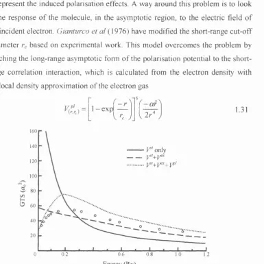
• The Polarisation Potential( is due to the long-range dipole moment induced by the polarisation of the molecule. Castellejo et al (1960) have shown that it is impossible to exactly treat the polarisation because all possible electronic molecular states must be included in the analysis of Schrodinger equation in order to represent the induced polarisation effects. A way around this problem is to look at the response of the molecule, in the asymptotic region, to the electric field of the incident electron. Gianturco et al (1976) have modified the short-range cut-off parameter based on experimental work. This model overcomes the problem by matching the long-range asymptotic form of the polarisation potential to the short- range correlation interaction, which is calculated from the electron density with the local density approximation of the electron gas
1 - exp
V '*c y
- o r
2
/
1.31160 140
V ' only
---pp' 120
100
TO
0 0.2 0.6 0.8 1.0 1 . 2
Energy (Ry)
Figure 1.3a Approxim ate theoretical results show the behaviour o f the grand total cross section (GTS) fitting for different interaction potentials {M orrison 1983) com pared with experim ental results (circles) for electron-H ; collisions o f G olden et ur/ (1966).
-where Vc may be the radius of the molecular charge cloud or an adjustable parameter used to fit the experimental cross section, and a is the polarisability o f the molecule.
These three physically distinct potentials are employed in the theoretical treatments with some degree of coupling found between the polarisation and exchange potentials. Figure 1.3a shows the effect o f each of the potentials on the fitting o f the experimental grand total cross section o f H2 molecule. Fitting resembles the experimental behaviour only when the three potentials are employed.
1.4 Methods of Theoretical Calculations
The non-spherical and multicentred nature of the molecules and the number of degrees of freedom involved in the electron-molecule interaction make it very difficult to calculate the equations and the potentials of the interaction. Therefore, different methods have been used in order to simplify the equations that govern the electron-molecule interaction. These methods will be listed with a brief description • The Born Approximation (BA) is used by replacing the scattered spherical wave
function by a plane one for large radial distance r. This leads to a Bom expansion of the scattering amplitude as powers in the potential strength, which makes it useful in the cases of a weak potential where only the first, and may be the second, term in Bom series is important. The modified scattering amplitude becomes
/ ( ^ ) = TTT" X “ i)f;(cos 9) + 1.32
Q(^) -2 i k
lin a k /=o
1 1 . ^ sin
3 2
0 ^ /) (cos 9)
1.33 V ^ y i>L (2/ + 3X2/ - 1)
tan S f = I U (,f^dr 1.34
0
9 l2/+1 »
1.35
where Cuo) represents the dipole-Bom approximation of the higher partial waves (/>L), a is the polarisability and Qq is the Bohr radius. Uq-) is the reduced spherical
symmetric potential The Bom approximation is the basis for most
scattering theories and modifications have been introduced to equation 1.32 (see
-chapter 4, section 4.2) to include more complicated scattering processes and the interaction potentials.
• Close Coupling Theory (CCT) truncates the higher terms in the expansion o f the total wave function in equation 1.22. The theory limits the expansion to the terms that are close in energy between the initial and final states i.e. before and after scattering. The truncated terms, even though they are inaccessible, still contribute to the scattering process as they are responsible for polarisation effects (see section 1.3 polarisation potential). However, a large number of coupled equations are generated in this approach due to small energy spacing between rotational and vibrational states, therefore, a full ro-vibrational close coupling approach is only feasible for low energy e-Hi collision.
A result of the CCT is the convergent close coupling (CCC) method developed by Bray and Stelbovics (1992) for solving the coupled equations. Convergence is tested by including an ever increasing set of target states in the CCT formalism. It is the CCC theory that describes the electron-atom scattering processes at all non- relativistic energies.
• Fixed Nuclei Approximation (FNA) was introduced by Massey ( 1930) to simplify the electron-molecule interaction by assuming that the inter-nuclear distance and the direction o f the molecular axis are fixed during the scattering process. Also assuming that the molecule is in the ground electronic state, the expansion in equation 1.22 is reduced to one term only. The calculations are computed frame by frame allowing for the change of the molecular orientation and the inter- nuclear separation, then the scattering amplitude is averaged over all possible states. The predictions of the FNA are in good agreement with experiments mainly at high incident electron energies (>100 eV).
Massey extended the theory to calculate rotational and vibrational cross
sections using what is called Adiabatic Nuclear Approximation (ANA), where the
• Frame transformation Theory(FTT) was formulated by F ana (1970) and Chang
and Fano (1972) to combine the advantages o f the CCT and FNA. The theory divides the electron scattering into two regions: 1) In the inner region the incoming electron is just inside the molecular electron cloud (r^), so it accelerates and sees a frozen nucleus. Thus for r < Vc the FNA is suitable for treating the collision process. 2) In the outer region the nuclear motion is included where the degree of coupling between different states is weak. Thus for r > the CCT is suitable to describe the scattering process. Then the FFT is utilised to bring the two regions together and matched at an arbitrary value (see Burke 1979 and
Buckley et al 1984 for details).
An alternative approach, known as the Angular Frame Transformation(AFT,
Collins and Norcross 1978), divides the orbital angular momentum space into two regions having angular momentum h at a common boundary. For / < // ANA is used and for / > // a suitable lab-frame calculation is used (full details in Norcross and
Collins 1982).
A number o f computational methods have been used to solve the electron- molecule scattering processes within the various theoretical approximations mentioned above. Many of these methods predict DCSs and GTSs very close to the experimental results and within the experimental errors. The main disagreement usually lies in the forward and backward scattering regions, as they were until recently experimentally inaccessible.
1.5 Analysis of Experimental Results
Many of the experiments that study DCSs and GTSs are limited in the ranges o f forward and backward scattering angles and the range of low incident electron energy. Therefore, two methods are used to fit the experimental results to overcome the absence of data in the experimentally inaccessible regions in order to obtain the integral cross sections (ICS) and the GTS.
• Phase Shift Analysis (PSA) employs the scattering amplitude o f equation 1.32 with and without modifications, which are listed in chapter 4 section 4.2. The Ci^e^
term (equation 1.33) is the contribution of the higher partial waves (/ > L) in the Bom approximation arising from the long-range interaction o f the induced-dipole