Article
Capital Structure Arbitrage under a Risk
Neutral Calibration
Peter J. Zeitsch
Calypso Technology Inc., San Francisco, CA 94105, USA; [email protected]; Tel.: +1-415-530-4000
Abstract: By reinterpreting the calibration of structural models, a reassessment of the importance of the input variables is undertaken. The analysis shows that volatility is the key parameter to any calibration exercise by several orders of magnitude. In order to maximize the sensitivity to volatility, a simple formulation of Merton’s model is proposed that employs deep out-of-the-money option implied volatilities. The methodology also eliminates the use of historic data to specify the default barrier thereby leading to a full risk neutral calibration. Subsequently, a new technique for identifying and hedging capital structure arbitrage opportunities is illustrated. The approach seeks to hedge the volatility risk, or vega, as opposed to the exposure from the underlying equity itself, or delta. The results question the efficacy of the common arbitrage strategy of only executing the delta hedge.
Keywords: merton model; structural model; credit default swap; capital structure arbitrage; algorithmic trading
JEL Classification: G12; G13
1. Introduction
The concept of capital structure arbitrage is well understood. Using Merton’s model of firm value [1], mispricing between the equity and debt of a company can be sought. Several studies have now been published [2-8]. As first explained by Zeitsch and Birchall [9], Merton models are most sensitive to volatility. Stamicar and Finger [10] showed the potential for exploiting that sensitivity by calibrating the CreditGrades model [11] to equity implied volatility in place of historic volatility. The results produced model implied CDS spreads that closely matched the actual traded 5-year CDS. Other studies [12-14] have subsequently been published which agree with the findings in [10] across a broad cross section of credits.
Within arbitrage studies, the calculation of asset volatility has not been consistently treated although the trend is generally towards sourcing implied volatility data. Yu [2] calibrated to a 1000-day historic volatility. Balazs and Imbierowicz [3] also employed historic volatilities. Baljum and Larson [4] calibrated the capital structure to a one month, at-the-money put implied volatility. Wojtowicz [5] computed the daily market implied volatility by solving for the model CDS premium that replicated the actual market CDS spread before taking a 100-day moving average of the resulting volatilities. Ju et. al. [6] adopt a volatility curve applied to a 1000-day historic volatility to introduce calibration flexibility. Huang and Luo [7] employed call option implied volatilities that underwent a least square error minimization.
employing this model over, say, the commercially available and widely used, KMV model [15] nor other models such as Leland and toft [16] or Geske and Johnson [17-18].
The aim of this study is to eliminate the use of historic data thereby improving the model’s responsiveness. To achieve this, calibration to deep out-of-the money put volatilities will be proposed using a basic Merton model. A new technique is then used to explicitly derive the default barrier. The methodology requires solving for the default threshold numerically, point by point, as the asset value where the market capitalization of the company asymptotes to zero. This naturally maintains the risk neutrality. The desire is to improve the responsiveness of the default probability calculation. It is well documented that Merton models often fail to replicate the outright magnitude of the CDS spread. With the enhancements outlined here, it will be shown that very close agreement between the traded CDS and the synthetic CDS are consistently possible. As first mentioned in [15], historically the credit risk of financial institutions has been difficult to model. That limitation is overcome here due to the focus on modeling the volatility.
The close agreement that results between the synthetic CDS and the traded contract forms the basis for the approach to identify capital structure arbitrage opportunities. Divergence between the synthetic and the traded CDS can still occur as sentiment may differ between the equity and credit markets for a given company. Trading a corporate’s equity against their debt is the basic technique of Capital Structure Arbitrage. However, all studies published to date only consider delta-hedging or trading the underlying equity itself against the CDS. As outlined in [9], the sensitivity to volatility, or vega, can be several orders of magnitude greater than the delta. Here we shall show that the main driver of the arbitrage strategy should be to trade the CDS against the equity implied volatility; not the stock itself. In fact, the equity or delta hedge is largely ineffectual when compared to the vega hedge. This result is also new. We then illustrate a volatility hedging technique with several case studies to show the effectiveness of focusing the hedging strategy on the implied volatility. This is then extended and back tested across all applicable CDS.
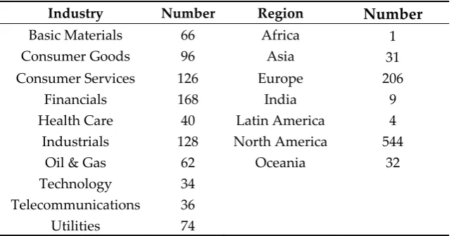
As summarized in Table 1, 830 credits are covered with data from January 2004 until December 2011. The companies are spread across all industries and geographies. This encompasses the universe of CDS contracts where an active equity option market also exists. It includes the liquid pre-Lehman market, the Lehman default itself and the subsequent European debt crisis. The volatility hedging strategy will be run against all 830 obligors across the entire time period. Summary statistics of the performance of the strategy, across the full universe of credits under consideration, are then presented.
Table 1. Credit Breakdown by Industry and Region1
Industry Number Region Number
Basic Materials 66 Africa 1
Consumer Goods 96 Asia 31
Consumer Services 126 Europe 206
Financials 168 India 9
Health Care 40 Latin America 4
Industrials 128 North America 544
Oil & Gas 62 Oceania 32
Technology 34 Telecommunications 36
Utilities 74
1 Classifications are those used by Markit
2. Model Description
crucial difference from all other models is the ability to calibrate risk neutrally thereby eliminating the need for historic data; in particular for calculating the default barrier.
Following [1], assume two classes of securities, namely equity and debt. The equity pays no dividends and the bond is due to be repaid at time T. Define
V
tas the value of the assets, andσ
Vas the asset volatility. In the Merton framework, the firm’s assets follow the geometric Brownian motion
dV
t=
rV
tdt
+
σ
VV
tdW
t,
(1)Where r is the asset drift due to risk-neutral interest rate dynamics and
dW
tis a standard Wiener process. The traded securities are S, the observed value of a company’s market capitalization (or share price), and a defaultable bond B, with maturity T. The payment to shareholders at time t is given by
S
=
max
(
V
t−
B
,
0
)
. (2)Market Capitalization is therefore given by the standard Black-Scholes formulation,
C
BS, as
S
C
(
V
t Vr
T
B
)
BS
,
σ
,
,
,
=
=
V
tN
(
d
1)
−
Be
−rTN
(
d
2)
, (3) whereT
T
B
e
V
d
V V rT tσ
σ
2
1
)
/
ln(
1
=
+
,T
d
d
2=
1−
σ
Vand N(..) is the Gaussian distribution. The default time within the model is calculated as the first hitting time for the default barrier. This is defined as
τ
=
min
[
t
:
V
t≤
B
′
( )
t
,
T
]
, (4)where
B
′
(
t
,
T
)
is the instantaneous default point for the bond at time t.Equity is a market observable. Total liabilities are obtained directly from an issuer’s balance sheet. The remaining unknowns are then the value of the firm’s assets and the asset volatility. Returning to (2), assume that an equity volatility exists, we then have that
dS
≈
S
σ
SdW
. (5)On the other hand, applying Ito’s lemma to (2) gives
dW
V
V
C
dt
dS
t Vt BS
σ
∂
∂
+
=
(...)
. (6)Equating (5) and (6), we find that
t BS t V S
V
C
S
V
∂
∂
=
σ
σ
. (7)There are two boundary conditions that
V
t must satisfy, namely)
,
(
|
0B
t
T
V
t S==
′
, (8)( )
t
T
B
S
>>
′
,
,S
V
t→
1
and
1
→
∂
They represent the behavior of
V
tnear default and also when well capitalized. To the first order, (8) givesS
S
V
T
t
B
V
t∂
∂
+
′
≈
(
,
)
.The simplest expression that will then satisfy (8) and (9) is
)
,
(
t
T
B
S
V
t≈
+
′
. (10)Substituting (10) into (7) yields
)
,
(
t
T
B
S
S
S V′
+
=
σ
σ
. (11)Equation (11) is the basic representation of the asset volatility as derived in CreditGrades [11]. However, CreditGrades subsequently holds the default barrier constant and models the recovery as a historically calibrated log-normal variable. In fact, this is not needed. Equation (8) already defines the default barrier.
The boundary condition (8) should also hold in the limit or
V
tB
( )
t
T
S
,
lim
0
=
′
→ . (12)
For senior unsecured debt, the market standard assumption for Loss Given Default, or LGD, is 60%. As an initial estimate for the default point take
( )
t
T
B
T
t
B
1′
(
,
)
=
0
.
6
×
,
. (13)Substitute (13) into (11). Equation (12) can now be solved numerically by seeking an updated
( )
t
T
B
2′
,
such that[
B
2′
(
t
,
T
),
,
T
,
B
]
→
0
C
VBS
σ
. (14)Equations (11) and (14) are then iterated for
B
i′
(
t
,
T
)
where i=1, 2, … until the desired accuracy levelis achieved (here typically to within 1%). The advantage of this approach is that at any given time, the exact liabilities and the relationship to the default point cannot be known. However, using the option curve to determine
B
′
(
t
,
T
)
allows calibration to the market and captures the latest sentiment thereby minimizing arbitrary intervention. Consequently, the default point will move day on day and it is risk neutrally calibrated. This approach to implying the default point is new.Now following [15], the probability of default is the probability that the issuer’s assets will be less than the book value of the issuer’s liabilities when the debt matures. That is:
[
t t t]
t
P
V
B
t
T
V
V
p
=
≤
′
(
,
)
|
=0=
=
P
[
ln
V
t≤
ln
B
′
(
t
,
T
)
|
V
t=0=
V
t]
, (15) wherep
tis the probability of default at time t,V
twas given by (1) and was calculated inB
′
(
t
,
T
)
in (14). From (1) we have that
,
2
ln
ln
2
0
r
σ
t
σ
t
ε
V
V
t t V
+
v
−
+
=
= (16)and
σ
Vwas defined in (11). Substituting (16) into (15) gives
ln
(
,
)
2
ln
2T
t
B
t
t
r
V
P
p
V vt
t
≤
′
ε
σ
σ
≥
−
+
′
=
t
t
r
T
t
B
V
P
v V t2
)
,
(
ln
2 .Now
ε
~
N
( )
0
,
1
and as a result we can define the default probability in terms of the cumulative Normal distribution as
−
+
′
=
t
t
r
T
t
B
V
N
p
v V t tσ
σ
2
)
,
(
ln
2. (17)
From (17), the synthetic CDS is given by
(
)
(
)
= = −−
−
⋅
=
ni i i
n i i i i i
p
DF
DF
p
p
LGD
CDS
1 1 11
, (18)
where
DF
iis the discount factor to the ith day andp
iis defined by (17). TheCDS
i, i=1..n, then formthe synthetic CDS time series. Any CDS contract requires a constant LGD assumption. As an initial estimate, LGD=60%, which is the market default. However, the LGD represents a degree of freedom that can be calibrated in order to reduce the pricing error between the synthetic CDS and the traded contract. Here, the LGD is scaled to minimize, on average, the magnitude of the synthetic versus the traded 5-year CDS. The LGD is calibrated once where 0<LGD<1 and then held constant. Yu [2] employed a similar technique by calibrating to minimize the sum of squared errors of the first 10 days of the time series. Given that the aim is to model the liquid 5 year CDS, the maturity of the model, T, is also set to 5 years.
3. Model Calibration
Here equation (11) will be calibrated to a 1-month 10-delta put implied volatility. The justification is both theoretical and motivated by market observables. Following Merton [1], define the debt-holder’s payoff as
D
t. Then
D
t=
min
[
B
( )
t
,
T
,
V
t]
=
B
+
min
[
V
t−
B
( )
t
,
T
,
0
]
=
B
( )
t
,
T
−
P
BS[
V
t,
σ
v,
r
,
T
,
B
( )
t
,
T
]
. (19)t
V
and B(t,T) were defined in equations (1) and (4) respectively.P
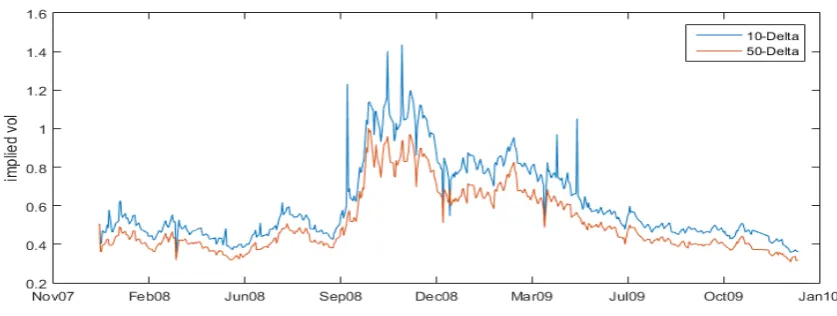
BSis the value of a put option analogous to (3). Hence debt-holders are long the face value of the bond and have sold a put option on the assets of the company. In theory, if the debt-holders bought back the put in (19), they would be hedged against default risk. In practice, this can only be achieved by buying CDS protection. Consequently, CDS can be thought of as a proxy for a put option on the assets of the firm. The value of the put option will vary depending on the value of the company’s equity. Large declines in the market capitalization will increase the value of the put option. The best indicator of such a decline will be the deep out-of-the money put implied volatilities.risk. In Figure 1, the average 10-delta and 50-delta 1-month put implied volatility is plotted through 2008 and 2009 for the companies listed in Table 1.
Figure 1. Average 1-Month 10-Delta versus 50-Delta Implied Equity Put Volatilities
In early 2008, the differential between the 10-delta and 50-delta put volatility was approximately 4 volatility points. By the last quarter of 2008 that difference was as large as 20. The peak difference of 60 volatility points occurred in September 2008 when Lehman defaulted. Only in late 2009 did the differential reduce back to 4 volatility points. The fact that the low delta volatilities can trade significantly higher and over a greater range of values than at-the-money volatilities will increase the variability and responsiveness of the default probability in (17). This will subsequently also be reflected in the calculation of the synthetic CDS. Using the lowest strike possible, or 10-delta, should therefore be the calibration choice. All volatility data was sourced from Bloomberg. The Bloomberg data series for the one-month maturity is the deepest. There are data for the three-month maturity but they are not as consistent. Beyond three-months, Bloomberg has no reliable data – hence the use of the 1-month 10-delta put volatility. This reflects the general open interest that can be seen in the market.
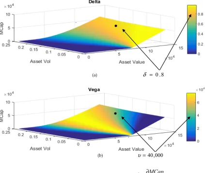
The choice of the implied volatility is crucial. Consider Figure 2. It shows the sensitivity for Bay Moteren Werke, or BMW, as the market capitalization moves against the underlying asset price and also against the asset volatility. The point on each surface shows the equity-liabilities relationship as of late 2011. The color of each plot represents the magnitude of each sensitivity. The value of each sensitivity can be ascertained by matching the color of the region where the point is located to the scale next to each chart. Reading off the charts, we can see that delta = 0.8 and vega = 40,000. In other words, the sensitivity to asset volatility is five orders of magnitude greater than the sensitivity to asset value. The difference in the magnitude of the sensitivities holds across all combinations of asset value and asset volatility.
The relative magnitudes of delta and vega is an observation that holds for all issuers. Table 2, shows the breakdown of delta and vega, in late 2011, by industry and geography, for the credits from Table 1. Putting aside the one credit from Africa, all names show at least a differential of 4 orders of magnitude between delta and vega. The largest discrepancy is for financials which shows a difference of 6 orders of magnitude. The heavy model dependence on volatility is a key reason that financial institutions have not performed well historically in Merton models. Financials are often excluded from analyses [2,5,13] as their capital structures have posed challenges. This will be exacerbated if the model is not fully calibrated risk neutrally to the most sensitive volatility, i.e. the 10-delta put.
(a)
δ
=
0
.
8
(b)
υ
= 40,000Figure 2. BMW sensitivities from equation (3) for: (a) Delta, or
Assets
MCap
∂
∂
=
δ
and (b) Vega, orAssetVol
MCap
∂
∂
=
υ
where MCap is the Market Capitalization (in millions), Assets represents the assetvalue of the company (in millions) and AssetVol is calculated in equation (11).
Table 2. Model Sensitivity Breakdown by Industry and Region1
Industry Mean
Delta
Mean
Vega Region
Mean Delta
Mean Vega
Basic Materials 0.94 3,525 Africa 0.87 111
Consumer Goods 0.92 37,411 Asia 0.91 63,935
Consumer Services 0.90 11,910 Europe 0.87 107,341
Financials 0.83 262,324 India 0.93 1,331
Health Care 0.95 3,054 Latin America 0.94 26,839
Industrials 0.93 4,967 North America 0.92 37,045
Oil & Gas 0.96 5,462 Oceania 0.94 40,625
Technology 0.95 3,256
Telecommunications 0.94 6,371
Utilities 0.94 7,330
4. Model Output
To illustrate the model’s performance, the output for four different credits from Europe, Asia and North America are shown in Figures 3-6. The companies in question are BMW, which continues the calibration exercise from the previous section, Boeing Co., Hutchison Whampoa and Hartford Financial Services. Here the choice of a financial institution is deliberate. As discussed in the previous section, such companies historically have proven difficult to calibrate in the Merton framework. However as given in Table 1, financials represent the largest percentage of credits that are applicable to this approach. Hence removing them significantly decreases the analysis opportunities. Here financial institutions are not excluded. With the risk-neutral model formulation derived earlier, the modelling limitations are overcome and good agreement between the synthetic CDS and the traded 5-year contract can be achieved. The ability for the model to replicate financial CDS is also new.
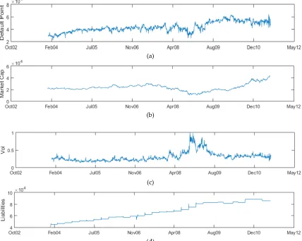
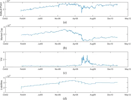
To illustrate the default barrier calculation, in Figure 3 the default point for BMW is calculated using equation (14) and plotted against the company’s market capitalization, asset volatility and liabilities through time. The charts show that the default point responds generally linearly versus the market capitalization and liabilities. The spike in asset volatility corresponding to the Lehman default significantly reduced the default barrier. In isolation, a lower default barrier would be interpreted as a reduction in default risk. In effect the rise in volatility is interpreted by the Merton model as an increase in the potential for the asset value of the company to grow – or the ability of the company to trade their way to higher profits. This needs to be coupled with the drop in market capitalization and the increase in leverage leading into 2008 to produce a higher default probability. Similarly, in Figure 4 the default barrier for Hartford Financial Services is plotted. There is a sharp decrease in the default barrier corresponding to the Lehman default. The increasing leverage prior to 2008 and the post-Lehman equity sell-off coupled with the rise in implied volatility produce a substantial move in the default point.
(a)
(b)
(c)
(d)
Again, the net non-linear effect is an increase in the default probability. Specifying the default barrier independently using historic data, such as in [11], cannot produce this market responsiveness. This directly contributes to the ability to accurately model financial institutions. For completeness, Figure 5 shows the default barrier for Hutchison Whampoa and Boeing Co.
In Figure 6, the synthetic CDS, calculated using (17) is plotted against the actual 5-year, senior unsecured, CDS spread. For all four corporates, there is close agreement between the synthetic CDS and the traded contract; including for the financial institution in Figure 6(c). Both the shape and the outright magnitudes of the spreads are comparable.
(a)
(b)
(c)
(d)
Figure 4. Hartford Financial Services time series for (a) the Default Barrier, (b) Market Capitalization, (c) 10-Delta Implied Volatility, (d) Liabilities. (a), (b) and (d) are in USD millions.
(a)
(b)
(a)
(b)
(c)
(d)
This indicates that both the equity and debt markets are pricing efficiently. The close agreement between the Merton model and the traded CDS agrees with the findings of Stimcar and Finger [10] as well as Huang and Luo [7]. Both studies employed model variants of [11].
From a capital structure perspective, the key is to look for divergence between the synthetic and traded CDS. There is evidence of this separation in Figure 6(c) for Hartford Financial Services in mid-2009 and again in late 2010. The synthetic CDS led the traded CDS by tightening faster in both instances. Theoretically, as the least secured creditors, equity markets should react faster than debt investors thereby creating the trading opportunities as shown. That is the case for Hartford Financial. However post-Lehman, this is no longer the case. Rather than seeing the traded CDS converge to the synthetic CDS, the opposite can occur. Consequently, it is necessary to trade the capital structure completely to hedge this effect by either buying or selling volatility on the underlying stock against the CDS as required.
5. Capital Structure Arbitrage
All arbitrage studies to date [2-8] have employed a strategy of trading the CDS against the underlying equity itself using a hedge ratio that is derived in closed form from the model. In effect the authors use
S
CDS
∂
∂
=
δ
, (20)where S was defined in (2). As shown in Figure 6, the synthetic CDS is not smooth. Both [7] and [10] show similar behavior. The implication is that the calculation of (20) will contain noise and the hedge ratio will vary significantly, even alternating between positive and negative values. One answer is to adopt a dynamic hedging strategy to adjust the delta hedge which Huang and Luo explore in [7].
None of the authors of [2-8] consider basing the trading strategy on the implied volatility. There is no justification for this approach apart from the fact that the delta hedge was derived in CreditGrades [11] which is the predominant capital structure model used in studies. Also CreditGrades uses a 1000-day moving average historical volatility. Such a calibration will drastically reduce the responsiveness to the volatility as the daily updates to the asset volatility only have a small incremental effect. Hence volatility hedging will not appear to be as relevant.
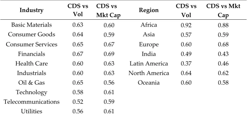
As shown in Table 3, there is no significant difference in the correlation between the CDS and the implied volatility nor the CDS with the market capitalization. Hence there is no empirical reason to favor one sensitivity over the other. The question is whether or not there is any justification for using an alternative to (20)? Table 2 indicated that the asset volatility was the key variable – not the
Table 3. Correlation of CDS vs Implied Volatility and CDS vs Market Capitalization1
Industry CDS vs
Vol
CDS vs
Mkt Cap Region
CDS vs Vol
CDS vs Mkt Cap
Basic Materials 0.63 0.60 Africa 0.92 0.88
Consumer Goods 0.64 0.59 Asia 0.57 0.59
Consumer Services 0.65 0.67 Europe 0.60 0.68
Financials 0.67 0.69 India 0.49 0.43
Health Care 0.60 0.63 Latin America 0.37 0.46
Industrials 0.60 0.63 North America 0.64 0.62
Oil & Gas 0.65 0.56 Oceania 0.60 0.58
Technology 0.58 0.61
Telecommunications 0.52 0.59
Utilities 0.56 0.61
1 Calculated from January 2004 until December 2011 using 5-year senior unsecured CDS and 10-delta implied
stock price. Hence the theoretical differential in the sensitivities suggests that the implied volatility should be considered.
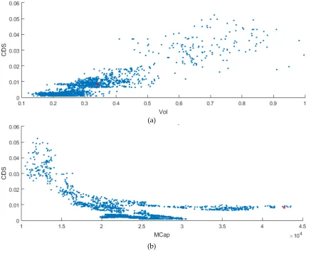
Returning to BMW, consider Figure 7. Here the 5-year CDS is plotted against both the 10-delta implied equity volatility and against the market capitalization. The plots span the entire time series from 2004 to the end of 2011. What is immediately apparent is that movement in the implied volatility corresponds to movement in the CDS whereas large moves in the market capitalization do not necessarily move the CDS. In fact, the BMW market capitalization drops from EUR 45BN to 15BN without an appreciable move in the CDS. Large CDS moves only occur when the market capitalization drops below EUR 15 BN. The difficulty of capturing stock moves against the CDS has also been reported in [20-21]. In effect, the realized movements in the market are reflecting the relative magnitudes of the delta and vega from Table 2.
(a)
(b)
Figure 7. Scatter Plot for BMW (a) 5-Year CDS versus 10-Delta Implied Volatility, (b) 5-Year CDS versus Market Capitalization. The red point indicates the company’s position as of the last data point.
In Table 4, empirical hedge ratios are calculated by regressing the CDS against the 10-delta put implied volatility and then against market capitalization for the entire cohort of 830 credits across the time series. Without fail, the CDS is significantly more sensitive to movements in the implied volatility than the market capitalization. In fact, Table 4 contradicts the delta-hedging strategy. The basic delta-hedging strategy used in [2-8] is to either sell protection on the CDS and short the stock or to buy protection on the CDS and buy the stock. If anything, the findings of table 4 contradict this approach. The delta-hedge in all cases is negative. Selling CDS protection and shorting the stock will, on average, always result in a loss on the equity leg.
for North America indicates that, on average, in order to hedge an 8bp move in the CDS, USD 100MN in equity needs to be held. In practice such positions are impossible to execute in the market either from the sheer volume of shares required or the amount of capital needing to be held to execute it. Trading the volatility offers a more effective hedge where the trader can actually ‘get set’ and it also captures the main responsiveness seen in the market.
Table 4. Empirical Sensitivity Breakdown by Industry and Region1
Industry Mean
Delta
Mean
Vega Region
Mean Delta
Mean Vega
Basic Materials -0.17 3.94 Africa 0.00 13.56
Consumer Goods -0.11 3.96 Asia -0.02 3.28
Consumer Services -0.51 10.00 Europe -0.56 3.43
Financials -0.27 4.6 India -0.02 6.35
Health Care -0.01 2.72 Latin America -0.08 4.90
Industrials -0.25 3.04 North America -0.08 5.00
Oil & Gas -0.03 3.18 Oceania -0.03 4.29
Technology -0.04 3.76 Telecommunications -0.03 2.42
Utilities -0.15 3.17
1 Mean Delta was calculated by regressing the CDS against the market capitalization for each credit per USD 1
million equivalent. For example, Consumer Goods shows a Mean Delta = -0.11 i.e. a 1.1bp move in the CDS corresponds to a USD 10 million move in the market capitalization. Likewise, for Consumer Goods, the Mean Vega = 3.96 i.e. a 3.96bp move in the CDS corresponds to a 1% volatility move (or 1 volatility point).
To reflect both the theoretical and empirical sensitivity, the main hedging tool to be used here is
σ
υ
∂
∂
=
CDS
, (21)where
σ
is the 10-delta implied put volatility. Furthermore, to reflect the noise inherent in the analytic calculation of (21), the hedge ratios will be calculated empirically. The model itself will only be used to signal arbitrage opportunities.To illustrate the debt-equity arbitrage, 3 case studies will be presented: Anadarko Petroleum Corporation (APC), Commonwealth Bank of Australia (CBA) and Peugeot SA (PEUGF) as representative examples of the approach.
5.1. Anadarko Petroleum.
As shown in Figure 8(a), following the Lehman default, there was a capital structure miss-alignment for APC in October 2008. The synthetic CDS had widened substantially further than the traded 5-year CDS. This indicates that the implied volatility is rich versus the CDS. Exploiting this requires selling puts on the equity itself versus buying protection on the CDS.
(a)
(b)
(c)
Figure 8. Andarko Pete Corp for (a) Synthetic CDS vs Traded 5-Year CDS from January 2004 to February 2009, (b) Scatter Plot of 5-Year CDS versus 10-Delta Implied Put Volatility with Regressed 3-Month Rolling Hedge Ratio and Mean Hedge Ratio from October 2008, (c) Scatter Plot of 5-Year CDS versus Market Capitalization with Regressed 3-Month Rolling Hedge Ratio and Mean Hedge Ratio from October 2008.
between the synthetic and traded CDS, the synthetic CDS is not ‘smooth’. This will introduce non-trivial noise into any theoretical calculation. From Figure 8(b), the empirical hedge ratio for APC varies across the time series with an average ratio of
CDS
≈
2
bps
/
vol
Δ
Δ
where vol=1%. In the second half of 2008, both the rolling 3-month numerical hedge and the long term average are of comparable magnitude thereby making (22) viable. Take a standard 5-year CDS contract with a notional of USD 10 MN. Define the dollar value sensitivity of the trade to a 1bp move in the CDS curve as the DV01. Using the standard ISDA CDS model [22], a quick calculation for APC shows that
4600
01
USD
DV
=
, (23)Multiplying (22) by (23) gives
200
,
9
USD
PV
CDSCDS
=
≈
Δ
Δ
υ
σ
,For late October 2008, seek liquid option contracts with the longest maturity profile. To satisfy this, choose the APC 25Jan 09 Puts at 30.62. Note that the option is close to at-the-money. The choice of strike was dictated by liquid available maturities and strikes following the Lehman default. A quick calculation shows that
υ
opt=
5
.
7
,where
υ
optis the dollar value of a single contract to a 1-point volatility shift. Each contract contains100 options which produces the following hedge
1600
7
.
5
9200
≈
=
hedge
.The full strategy is then
• Buy USD 10MN APC protection at 152bps.
• Sell 1600 contracts of APC 25 Jan 09 Puts at 30.62 with delta exchange.
The revenue from selling the puts is USD 1,200,000. From figure 8 (a), the synthetic and traded 5-year CDS had re-converged by mid-February 2009. In fact, the 5-year CDS had widened from 152bp to 239bp. The APC 1M ATM vol dropped from 120.25% to 60.75%. The equity price rallied from USD 30 to USD 40. Hence the P&L equals:
• CDS: USD 400,000 profit.
• Equity volatility: USD1,150,000 profit.
Hence a net profit of USD 1,550,000 results. This is an example where both legs converge and are profitable. In the next case study, the volatility position will provide a hedge against loss on the CDS leg.
5.2. Commonwealth Bank.
Now consider CBA. As shown Figure 9 (a), the synthetic CDS and the traded 5-year CDS were misaligned in March 2010. From Figure 9 (b),
000
,
15
USD
CDS=
υ
,per USD 10MN contract notional. With a more stable post-Lehman market, seek to trade low delta options. Hence take the 25-delta CBA 25 June 10 Puts at 53 where
9
.
8
AUD
opt=
υ
,which leads to the arbitrage hedge
1
,
800
935
.
0
9
.
8
000
,
15
≈
×
=
hedge
and 0.935 is the FX spot rate for the AUD. The trading strategy, executed in mid-April, is then:
• Sell USD 10MN protection on CBA at 74bp.
• (a)
(b)
(c)
Figure 9. CBA for (a) Synthetic CDS vs Traded 5-Year CDS from January 2004 until May 2010, (b) Scatter Plot of 5-Year CDS versus 10-Delta Implied Put Volatility with Regressed 3-Month Rolling Hedge Ratio and Mean Hedge Ratio from March 2010, (c) Scatter Plot of 5-Year CDS versus Market Capitalization with Regressed 3-Month Rolling Hedge Ratio and Mean Hedge Ratio from March 2010.
Following Figure 9(a), in May 2010, there was civil unrest in Greece. This led to a sell-off in risky assets. Hence by the end of the first week of May 2010 the 5-year CDS referencing CBA had widened to 118bps. The CBA 25-delta volatility had increased from 16.5% to 31.3%, producing the following P&L:
• CDS: USD 200,000 loss.
• Equity options: USD 300,000 profit.
• Net P&L: USD 100,000 profit.
convergence in the capital structure. Likewise, delta hedging would have been ineffectual. From March to May 2010, the underlying CBA share price only moved from AUD 55.6 in mid-march to 53 in the first week of May. As per [2-8], selling CDS protection requires shorting the stock as the hedge. In that case, the loss would have only been minimally offset by the movement in the share price. Figure 9 (c) confirms the general low sensitivity of the CDS to the share price.
5.3. Peugeot SA.
During 2010, arbitrage opportunities in the French auto-makers, Peugeot and Renault, developed due to rating downgrades from S&P and Moody’s. Both companies saw their ratings drop to sub-investment grade. This lead the CDS market wider despite a relatively stable equity market. As shown in Figure 10 (a), the synthetic CDS and the traded 5-year CDS were misaligned for the second time in June 2010.
(a)
(b)
(c)
Calculating the empirical hedge ratio gives
500
,
29
USD
CDS=
υ
,per USD 10MN contract notional. Figure 10 (b) shows a strong agreement between the 3-month and mean hedge ratios. With such a large delta, there is a need to cheapen the volatility hedge as much as possible. This is done by extending the maturity and decreasing the delta.
Consider the PEUGF 25 Sep P16; effectively a 3 month 10-delta option. Hence
95
.
1
EUR
opt
=
υ
,which leads to the arbitrage hedge
12
,
000
22
.
1
95
.
1
18000
≈
×
=
hedge
,where 1.22 is the FX spot rate for the EUR.
The trading strategy, executed in early June, is then:
• Sell USD 10MN protection on PEUGF at 344bp.
• Buy 12,000 contracts of PEUGF 25 Sep P17 with delta exchange.
Following Figure 10 (a), both the actual traded 5-year CDS and the synthetic CDS continued to tighten until converging in November 2010. The actual CDS tightened from 344bps to 213bp. The share price increased from 20.27 to 28.46. Likewise, volatility decreased by 10 points. Hence the options expired worthless. The resulting P&L was then:
• CDS: USD 600,000 profit.
• Equity options: EUR 330,000 loss.
• Net P&L: USD 270,000 profit.
Here the vega hedge was not required and expired worthless. That loss was offset by the gain in the CDS. However, the importance of hedging with a (relatively) inexpensive low-delta position was crucial to protecting against any volatility spike while keeping the overall cost of the volatility hedge low so as not to erode the P&L from the CDS position. Note that the delta-hedging strategy of selling protection on the CDS and shorting the stock would have resulted in a loss on the equity leg. In fact, as shown in Figure 10 (c), the relationship between the CDS and the equity is consistently negative.
6. Back Testing
The previous section outlined the basic capital structure arbitrage technique required to trade the 5-year CDS against the equity implied volatility. Here that process is automated to identify capital structure misalignments across the time series of all 830 applicable CDS from 2004 until the end of 2011. Define the L-2 distance function, D, as
(
)
−
=
i
traded i synthetic
i
CDS
CDS
D
, , 2 .The data from 2004 and 2005 are used to initially calibrate the model and to calculate the L-2 distance. Call this the historic differential. Similarly calculate the L-2 distance for the current trading month,
D
c. That is then calculated from January 2006 onwards. Likewise, D is updated to thepreceding month. Define the signal strength as the ratio of the current differential divided by the historic differential,
D D
Signal= c . (22)
CDS has deviated from the traded CDS based on the historical average. This is then an indicator of a capital structure misalignment. Given the relative positions of the synthetic and traded CDS, the arbitrage strategy is executed. Define a trade that buys CDS protection and sells volatility as “short” the credit (or “buying” protection on the CDS). Likewise define a trade that sells CDS protection and buys volatility, as being “long” the credit (or “selling” protection on the CDS).
Positions matching the top 10 signals are entered into with equal CDS trade notionals of USD 10 MN versus appropriatevega hedges determined from the empirical hedge ratio. All CDS positions were actively quoted in the market at the time of trading in a size of USD 10 MN – including during the Lehman default. Trades were held until the synthetic CDS converged with the traded contract or a maximum holding period of 6 months was reached. If a position was closed out, a new trade was entered into based on the strongest untraded signal given by (22). The daily P&L is shown in Figure 11 (a).
(a)
(b)
Figure 11. Back Testing: 2006 to 2011 for (a) Daily P&L and (b) Long versus short positions plotted against on-the-run CDX.NA.IG.
For the period from January 2006 to December 2011, we find:
• Percentage of winning trades: 70%.
• Percentage of losing trades: 30%.
• Percentage of re-converging trades: 80%.
• Maximum consecutive winners: 19.
• Maximum consecutive losers: 4.
• Number of long trades: 139.
• Number of short trades: 145.
• Percentage of the universe traded: 12%.
• Average annual return: USD 14MN.
An immediate observation is that only a small percentage of the available companies were actually traded. Recall that the arbitrage strategy seeks explicit misalignment in the capital structure as measured by the differential between the synthetic CDS and the actual 5-year CDS; or L-2 distance. Moreover, the dislocation should be significant versus the historic differential. At any point in time, most corporates do not display any misalignment. Hence the strategy is very selective. The largest drawdown was USD 1.2MN in December 2008. In general, profitable days outnumber the losses. Also the magnitude of the losses is smaller than the size of the profits. This is an indication of the effectiveness of the vega hedge. Actual market quotes, incorporating bid-offers, were used to calculate the P&L. Hence accurate transaction costs are included in the calculations. Given that the strategy was driven by the implied volatility, in both the sensitivity of the model and the trading strategy, that can be seen in the resulting P&L. Before the Lehman default, outright levels of volatility in the market were low. This is reflected in the low P&L. The period of highest volatility, 2008-2009, yields the highest returns. Other periods are commensurate.
The strategy is market neutral. In Figure 11 (b), trades are evenly split between buy and sell positions. The model tends to detect buy protection signals in a weakening market and sell protection opportunities when CDS spreads are tightening. The selection criteria favored credits with lower L-2 distances i.e. corporates where the synthetic and traded CDS were historically tightly coupled. Consequently, the percentage of positions where the capital structure re-aligned was high. Only a small number of trades actually exceeded the 6 month holding period.
7. Conclusions
All previous capital structure arbitrage studies have focused on trading the CDS against the underlying equity itself. The importance of the equity volatility in the arbitrage strategy has been largely ignored. Here a deep out-of-the-money put volatility was used to calibrate the structural model. Then by using a fully risk neutral calibration, in particular to derive the default barrier, very exact matches can be achieved between the synthetic CDS and the traded CDS contract. Misalignment between the synthetic and traded CDS will still occur when credit and equity markets diverge in opinion on the quality of an obligor – hence the arbitrage opportunities. By basing the trading strategy on the relationship between the implied volatility and the CDS, and deriving the hedge ratio empirically, an effective convergence strategy can be executed. The strategy required hedging the risk due to movement in the implied volatility not the underlying stock.
Acknowledgements: The author is grateful to Markit and Bloomberg for the use of their data. The 5-year senior unsecured CDS spread from Markit was used in all calculations. All other data were sourced from Bloomberg (share price, shares outstanding, total liabilities and interest rates). The research presented here was conducted over a period of time variously at ANZ Bank, DBS Bank and National Australia Bank. The author also thanks Calypso Technology Inc. for the use of their analytics in the back testing.
Conflicts of Interest: The author declares no conflict of interest.
References
1. Merton, R.C. On the Pricing of Corporate Debt: The risk structure of Interest Rates, J. Finance 1974, 29, 449-470.
2. Yu, F. How Profitable Is Capital Structure Arbitrage, Financ. Anal. J.2006, 62, 47—62.
3. Balazs, C.; Imbierowicz, B. How Efficient Are Credit Default Swap Markets? An Empirical Study of Capital Structure Arbitrage Based on Structural Pricing Models. 21st Australasian Finance and Banking Conference.
2008.
4. Bajlum, C.; Larsen, P. Capital Structure Arbitrage: Model Choice and Volatility Calibration. Copenhagen Business School and Denmark National Bank. Working Paper. 2008.
5. Wojtowicz, M. Capital Structure Arbitrage Revisited. Duisenberg School of Finance – Tinbergen Institute Discussion Paper. Working Paper. 2014.
6. Ju, H-S.; Chen, R-R.; Yeh, S-K.; Yang, T-H. Evaluation of Conducting Capital Structure Arbitrage Using the Multi-Period Extended Geske-Johnson Model, Rev. Quant. Fin. Account. 2015, 44, 89-111.
7. Huang, Z.; Luo, Y. Revisiting Structural Modeling of Credit Risk – Evidence from the Credit Default Swap (CDS) Market, J. Risk Financial Manag.2016, 9, 3.
8. Duarte, J.; Longstaff, F.A.; Yu, F. Risk and Return in Fixed Income Arbitrage: Nickels in front of a Steamroller? Rev. Financ. Stud.2007, 20, 769 – 811.
9. Zeitsch, P.; Birchall, K. Pricing Credit Risk, Asia Risk2003, December.
10. Stamicar, R.; Finger, C.C. Incorporating Equity Derivatives into the CreditGrades Model. J. Credit Risk2006,
2, 1-20.
11. Finkelstein V.; Pan, G.; Lardy, J.P.; Ta, T.; Tierney, J. CreditGrades Technical document, Risk Metrics. 2002.
12. Byström, H. CreditGrades and the iTraxx CDS Index Market. Financ. Anal. J. 2006, 62, 65-76.
13. Cao, C.; Yu, F; Zhong, Z. Pricing Credit Default Swaps with Option-Implied Volatility, Financ. Anal. J.2011,
67, 67—76.
14. Cao, C.; Yu, F; Zhong, Z. The Information Content of Option-Implied Volatility for Credit Default Swap Spreads, J. Financ. Mark.2010, 13, 321—343.
15. Crosbie, P.; Bohn, J. Modeling Default Risk. Moody’s KMV, 2003.
16. Leland, H.; Toft, K.B. Optimal Capital Structure, Endogenous Bankruptcy and the Term Structure of Credit Spreads. J. Finance1996, 51, 987-1019.
17. Leland, H. Corporate Debt Value, Bond Covenants and Optimal Capital Structure. J. Finance1994, 49, 1213 – 1251.
18. Geske, R. The valuation of Corporate Liabilities as Compound Options, J. Financ. Quant. Anal. 1977, 5, 541-552.
19. Geske, R.; Johnson, H. The Valuation of Corporate Liabilities as Compound Options: A Correction, J. Financ. Quant. Anal. 1984, 19, 231-232.
20. Norden, L.; Weber, M. The Co-Movement of Credit Default Swap, Bond and Stock Markets: An empirical analysis. Europ. Financ. Manag.2009, 15, 529 – 562.
21. Kapadia, N.; Pu, X. Limited Arbitrage between Equity and Credit Markets, J. Financ. Econ. 2012, 105, 542-564.
22. ISDA CDS model, www.cdsmodel.com. 2009.