Finite difference scheme with spatial fourth order accuracy for a class of time fractional parabolic equations with variable coefficient

(1)

R E S E A R C H

Open Access

Finite difference scheme with spatial

fourth-order accuracy for a class of time

fractional parabolic equations with variable

coefﬁcient

Qinghua Feng

1*

_{and Fanwei Meng}

2

*_{Correspondence: [email protected]} 1_{School of Science, Shandong} University of Technology, Zhangzhou Road 12, Zibo, Shandong 255049, China Full list of author information is available at the end of the article

Abstract

In this paper, we establish a finite difference scheme for a class of time fractional parabolic equations with variable coefficient, where the time fractional derivative is defined in the sense of the Caputo derivative. The local truncating error, unique solvability, stability, and convergence for the present scheme are discussed by use of the Fourier analysis method, which shows that the present finite difference scheme is unconditionally stable and possesses spatial fourth-order accuracy. Theoretical analysis is supported by two numerical examples, and the maximum errors and the convergence order are checked.

Keywords: time fractional parabolic equation; variable coeﬃcient; high-order diﬀerence scheme; unconditional stability

1 Introduction

Nonlinear partial differential equations are widely used to describe many complex phe-nomena in various fields including the scientific work and engineering fields. In particu-lar, fractional differential equations (FDEs) containing the fractional derivative are widely used as models to express many important physical phenomena such as fluid mechan-ics, plasma physmechan-ics, classical mechanmechan-ics, quantum mechanmechan-ics, nuclear physmechan-ics, solid state physics, chemical kinematics, chemical physics, and so on. For the basic theory and differ-ent applications of derivatives and integrals of fractional order in various domains, we refer the readers to []. In order to better illustrate the described physical phenomena, we need to obtain the solutions of FDEs. However, the analytical solutions are usually difficult to obtain. So numerical solutions for FDEs have been paid much attention by many authors, and so far many numerical methods for obtaining the approximate solutions of FDEs have been developed. Among the numerical methods, the finite difference method is the most widely used method to solve FDEs, and many types of FDEs have been solved so far by use of explicit and implicit finite difference methods, compact finite difference methods, alter-nating direction implicit difference methods, and so on. For example, in [, ], the authors developed two valid difference schemes for the fractional advection-diffusion equations and proved the stability and convergence, whereas in [–], difference schemes for the

(2)

fractional advection-dispersion equations were established. In [–], compact finite dif-ference schemes were proposed to solve the fractional advection-dispersion equations, the fractional convection-dispersion equations, and the fractional diffusion equations re-spectively, whereas in [], a compact alternating direction implicit scheme for a class of two-dimensional time fractional diffusion equations was developed. In [–], vari-ous finite difference schemes for the fractional subdiffusion equations and the fractional diffusion-wave equations were established.

Among the works mentioned, we notice that most of the current research on numeri-cal methods for solving FDEs are concerned with the constant-coefficient case, and rel-atively less attention has been paid to the cases with variable coefficient. In [, ], the authors presented compact finite difference schemes with convergence orderO(τ–α+h₎ ( <α< ) for fractional subdiffusion equation with spatially variable coefficient, whereas Wang et al. [] proposed a Petrov-Galerkin finite element method for variable-coefficient fractional diffusion equations and proved the well-posedness and optimal-order conver-gence of this method. Chen et al. [] presented a fast semiimplicit difference method with convergence orderO(τ+h) for a nonlinear two-sided space-fractional diffusion equation with variable diffusivity coefficients and also developed a fast accurate iterative method by decomposing the dense coefficient matrix into a combination of Toeplitz-like matri-ces, whereas Wang [] established a compact finite difference method with convergence orderO(τ–α₊_τ₊_h_{) ( <}_α_{< ) for a class of time fractional convection-diffusion-wave} equations with variable coefficients.

In this paper, we consider the following time fractional parabolic equation with spatially variable coeﬃcient and nonhomogeneous source term:

C D

α tu(x,t) =

∂ ∂x

a(x)∂ _u(x,_t)

∂x

+f(x,t),  <α< , ()

which is subject to the initial and periodic boundary value conditions

u(x, ) =ϕ(x), x∈R,

u(x,t) =u(x+L,t), x∈R,t∈[,T], ()

whereC

Dαtu(x,t) =(–α)

t 

u_t(x,s)

(t–s)α dsdenotes the Caputo derivative of orderαonu(x,t),

Lis the period ofu(x,t) with respect to the variablex, anda(x) is assumed to be smooth enough and satisfya(x)≤L< .

The aim of this work is to develop a finite difference scheme with spatial fourth-order accuracy for the above problems. First, in Section , we give the derivation of the finite difference scheme for solving problems ()-(). Then, in Sections  and , we carry out theoretical analysis including unique solvability, stability, and convergence for the finite difference scheme by use of the Fourier analysis method. In Section , numerical experi-ments are given to support the theoretical analysis. Some conclusions are presented at the end of this paper.

2 The ﬁnite difference scheme

(3)

τ ={tn|≤n≤N}, (i,n) = (xi,tn), and then the domain [,L]×[,T] is covered by

h×τ. LetVh={un_i|≤i≤M, ≤n≤N}be the grid function on the meshh×τ, U_in=u(xi,tn_{) and}_un

i denote the exact and numerical solutions at the point (i,n), respec-tively, andUn_{= (U}n

The proof of Lemma  can be completed by applying the expansion of Taylor’s formula to the right term of Eq. ().

In order to establish the ﬁnite diﬀerence scheme for solving problems ()-(), we rewrite Eq. () in the following form:

(4)

wherea_i=a(xi),ai=a(xi),f_in=f(xi,tn_),_ψ

So the ﬁnite diﬀerence scheme approximating Eq. () at the point (i,n) under conditions () can be established as follows:

⎧

3 Unique solvability of the difference scheme

In this section, we research the unique solvability of the diﬀerence scheme () by use of the Fourier analysis method. To this end, the ﬁrst equation in () can be rewritten as follows:

Letvn_(x),_zn_{(x) be two periodic functions with period}_{L, and denote their restrictions on} [,L] by

Furthermore, let the expansions of the Fourier series ofvn(x) andzn(x) be

(5)

where

andjdenotes the imaginary unit. Deﬁne the discreteLnorm by

un_=

Then the following equalities hold according to the Parseval identity:

un_=

Substituting () into () yields that

∞

Sinceai< , we can deduce thatyis indeed nondecreasing with respect tocos(βh), which implies thaty≤ai< .

Due to the previous observations, we can get that

(6)

Multiplying both sides of () byexp(–βxj) and integrating from  toL, we get that

(s–y–yj)vnl = n–

k=

bn_kvk_l + hzn_l, l= ,±,±, . . . ,±∞. ()

In order to prove the unique solvability of the finite difference scheme (), we only need to prove that there is only the zero solution for the following homogeneous difference equation:

⎧ ⎪ ⎨ ⎪ ⎩

τ–α (–α)u

n

i –aiψuni –aiψuni = , ≤n≤N, u_i =ϕ(xi),

un_i =un_i_±_M, ≤i≤M, ≤n≤N.

()

On the other hand, similarly to the process above, the following equation can be obtained due to ():

(s–y–yj)vnl = , ()

which implies thatvn

l =  since|s–y–yj|=

(s–y)+y> . Furthermore,vn(x) =  and un

= , which implies thatuni = ,i= , , . . . ,M. So there is only the zero solution for the homogeneous diﬀerence equation (). Then we have the following theorem.

Theorem  The ﬁnite diﬀerence scheme()is uniquely solvable.

4 Stability and convergence

In this section, we analyze the stability and convergence for the ﬁnite diﬀerence scheme ().

Lemma  For Eq. (),we have the estimate

vn_l≤( +τ)nv_l+max

≤s≤nz s

l. () Proof We use mathematical induction method to prove ().

Whenn= , due to (), we obtain

(s–y–yj)vl=bvl+ hzl=svl + hzl,

which implies that

v_l=sv 

l + hzl s–y–yj

≤ s

(s–y)+y

v_l+ h 

(s–y)+y

z_l

≤v_l+( –α)ταz_l

(7)

Ifτ≥, thenτα_≤_τ _≤_{ +}_τ_{, whereas}_τα_≤__≤_{ +}_τ _{if  <}_τ _{< . So}_τα_≤_{ +}_τ _for_τ _{> .}

which implies that () holds. So the proof is complete according to the mathematical

induction method.

Theorem  The diﬀerence scheme()is absolutely stable on the initial value and the right

(8)

Proof From Lemma  and the Parseval identity we deduce that

Then, combining () and (), we deduce that

τ–α Similarly to the deduction of (), we have

un–un_≤eTu–u_+max

which implies that small vibration from the initial value or the right source term also leads to small variation in the solutions. So the ﬁnite diﬀerence scheme () is absolutely stable on the initial value and the right term. The proof is complete.

Remark  Ifa(x) > , then from the expression ofy we can deduce thaty> , which implies that Lemma  may not hold, and then the ﬁnite diﬀerence scheme () may be conditionally stable or be unstable.

In order to investigate the convergence of the ﬁnite diﬀerence scheme (), letε_in=Un i –

Similarly to the deduction of (), we can get that

(9)

where

C= eT

( –α)

 –α

 + –α  –α –

 + –α max

t≤t≤tn

u_t(x,t),

C=eT

 max≤x≤L

u()_x (x,t)+  max≤x≤L

u()_x (x,t)

.

So we arrive at the following theorem.

Theorem  The ﬁnite diﬀerence scheme() is convergent with the fourth-order conver-gence in spatial direction.

5 Numerical experiments

In this section, we carry out numerical experiments to support the theoretical results. For further use, lete(τ,h) =max≤n≤N|Un–un|andRateh=ln(e(τln,h(h)//he(τ),h)) denote the

maxi-mum error and the convergence order in spatial direction, respectively.

Example  Consider problems ()-() with an exact analytical solution u(x,t) = (t₊ )sin(πx),L= , which satisﬁes

⎧ ⎪ ⎪ ⎪ ⎨ ⎪ ⎪ ⎪ ⎩

a(x) = –(x+ ),

u(x, ) =ϕ(x) =sin(πx), f(x,t) = –π_x(t_{+ )}_cos_(_π_x)

+ [π_(t_{+ ) + }_π_x_(t_{+ ) +}t–α

(–α)]sin(πx).

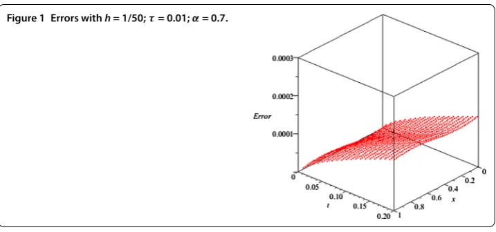
In Figures -, the approximating errors and states between the exact solutions and nu-merical solutions are shown, whereas in Tables  and , the maximum errors and conver-gence orders in spatial directions witht∈[, .] are listed.

Example  Consider problems ()-() with an exact analytical solutionu(x,t) = (t₊ )sin(πx),L= , and

⎧ ⎪ ⎨ ⎪ ⎩

a(x) = –(x+ ),

u(x, ) =ϕ(x) =sin(πx),

f(x,t) = –πx(t_{+ )}_cos_(_π_{x) + [}_π_(t_{+ ) + }_π_x_(t_{+ ) +} t–α

(–α)]sin(πx).

(10)

Figure 2 Comparison between exact solutions and numerical solutions withα= 0.7,h= 1/50,

τ= 0.01,t= 0.2.

Table 1 The maximum errors and convergence order in spatial direction withτ= 10–3

h α= 0.9 α= 0.7 α= 0.5

e(τ, h) Rateh e(τ, h) Rateh e(τ, h) Rateh 1

28 6.90559×10

–5 _– _7.52208_×₁₀–5 _– _7.62869_×₁₀–5 _–

1

26 9.27939×10

–5 _3.98694 _1.02720_×₁₀–4 _4.20438 _1.05053_×₁₀–4 _4.31756 1

24 1.28154×10

–4 _4.03352 _1.40144_×₁₀–4 _3.88122 _1.40817_×₁₀–4 _3.66048 1

22 1.81614×10

–4 _4.00691 _2.00611_×₁₀–4 _4.12245 _2.06562_×₁₀–4 _4.40332 1

20 2.65113×10

–4 _3.96890 _2.92642_×₁₀–4 _3.96161 _3.03546_×₁₀–4 _4.03874

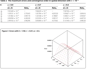
Table 2 The maximum errors and convergence order in spatial direction withτ= 10–2

h α= 0.9 α= 0.7 α= 0.5

28 7.81649×10

–5 _– _7.84420_×₁₀–5 _– _7.94746_×₁₀–5 _–

1

26 1.03531×10–4 3.79243 1.05784×10–4 4.03520 1.05607×10–4 3.83616 1

24 1.41482×10–4 3.90170 1.43168×10–4 3.78067 1.44821×10–4 3.94507 1

22 2.05058×10–4 4.26520 2.01039×10–4 3.90157 2.14181×10–4 4.49733 1

20 2.99163×10–4 3.96246 3.05069×10–4 4.37562 3.13140×10–4 3.98520

Figure 3 Errors withh= 1/40;τ= 0.01;α= 0.5.

(11)

Figure 4 Comparison between exact solutions and numerical solutions withα= 0.5,h= 1/40,

τ= 0.01,t= 0.1.

Table 3 The maximum errors and convergence orders in spatial direction withτ= 10–3

h α= 0.9 α= 0.7 α= 0.5

28 6.91107×10

–5 _– _7.52059_×₁₀–5 _– _7.63106_×₁₀–5 _–

1

26 9.28465×10

–5 _3.98390 _1.02705_×₁₀–4 _4.20514 _1.03136_×₁₀–4 _4.03963 1

24 1.28210×10

–4 _4.03182 _1.40131_×₁₀–4 _3.88184 _1.40804_×₁₀–4 _4.40284 1

22 1.81665×10–4 4.00520 2.00594×10–4 4.12254 2.06535×10–4 3.88945 1

20 2.65168×10–4 3.96811 2.92628×10–4 3.96201 3.03532×10–4 4.06486

Table 4 The maximum errors and convergence orders in spatial direction withτ= 10–2

h α= 0.9 α= 0.7 α= 0.5

28 7.49956×10

–5 _– _7.52514_×₁₀–5 _– _7.68218_×₁₀–5 _–

1

26 9.95995×10

–5 _3.82860 _1.02577_×₁₀–4 _4.18013 _1.03467_×₁₀–4 _4.01801 1

24 1.37506×10–4 4.02926 1.39977×10–4 3.88373 1.43168×10–4 4.05737 1

22 2.01028×10–4 4.36463 1.97818×10–4 3.97498 2.12006×10–4 4.51202 1

20 2.95158×10–4 4.02966 3.01869×10–4 4.43439 3.11013×10–4 4.02076

Example  Consider problems ()-() with an exact analytical solutionu(x,t) = ( +t+

t–α₎_ln₍_cos_x_{+ ),}_L_{= }_π_{, and}

⎧ ⎪ ⎪ ⎪ ⎪ ⎪ ⎪ ⎪ ⎪ ⎪ ⎨ ⎪ ⎪ ⎪ ⎪ ⎪ ⎪ ⎪ ⎪ ⎪ ⎩

a(x) = –ex– ,

u(x, ) =ϕ(x) = ln(cosx+ ),

f(x,t) = [t_(––α_α₎+(–_(–α)t–α_α₎ ]ln(cosx+ ) +ex_[(+t+t–α)sinx

+cosx –

(+t+t–α)cosxsinx

(+cosx) –(+t+t –α₎_sin_x

(+cosx) ]

+ (ex_{+ )[}(+t+t–α₎_cos_x

+cosx +

(+t+t–α_)(_sin_x_–_cos_x₎

(+cosx)

–(+t+_(+t–α_cos)cos_x₎xsinx–

(+t+t–α)sinx (+cosx) ].

(12)

Table 5 The maximum errors and convergence orders in spatial direction withτ= 10–3and

t∈[0, 0.05]

h α= 0.9 α= 0.8 α= 0.7

18 9.37861×10

–4 _– _2.14166_×₁₀–3 _– _5.11973_×₁₀–3 _–

1

16 1.50810×10–3 4.03287 3.34524×10–3 3.78626 8.33874×10–3 4.14160 1

14 2.55210×10–3 3.93964 5.72571×10–3 4.02473 1.45425×10–2 4.16504 1

12 4.65456×10–3 3.89833 1.03879×10–2 3.86424 2.68133×10–2 3.96899 1

10 9.42235×10–3 3.86810 2.11810×10–2 3.90773 5.31652×10–2 3.75439

Table 6 The maximum errors and convergence orders in spatial direction withτ= 10–4and

t∈[0, 0.01]

h α= 0.9 α= 0.8 α= 0.7

18 1.44527×10–3 – 3.49475×10–3 – 5.11973×10–3 – 1

16 2.39382×10–3 4.28410 5.47831×10–3 3.81663 8.51837×10–3 3.78163 1

14 4.25691×10–3 4.31099 9.16482×10–3 3.85359 2.25842×10–2 3.96621 1

12 7.87254×10

–3 _3.98855 _1.71871_×₁₀–2 _4.07904 _4.42381_×₁₀–2 _4.36155 1

10 1.60094×10

–2 _3.89308 _3.79037_×₁₀–2 _4.33788 _8.84836_×₁₀–2 _3.80224

Figure 5 The exact solutions withh= 1/40;

τ= 10–4_;_α_{= 0.85.}

Example  Consider problems ()-() with an exact analytical solution u(x,t) = ( + t–α₎₍_cos_x_{+ )e}cosx_,_L_{= }_π_{, and}

⎧ ⎪ ⎪ ⎪ ⎪ ⎪ ⎪ ⎪ ⎪ ⎪ ⎪ ⎪ ⎨ ⎪ ⎪ ⎪ ⎪ ⎪ ⎪ ⎪ ⎪ ⎪ ⎪ ⎪ ⎩

a(x) =sinx– ,

u(x, ) =ϕ(x) = (cosx+ )ecosx,

f(x,t) =(–_(–α)t–α_α₎ (cosx+ )ecosx_{) –}_ecosx_cos_x

×[sinx+ cosxsinx– sinx– ( +cosx)sinx+ (( +cosx))sinxcosx + ( +cosx)sinx] –ecosx₍_sin_x_{– )[}_cos_x_{– }_sin_x_{– }_cos_x_sin_x

+ cos_x_{+ }_sin_x_{+ ( +}_cos_x)_sin_x_{– ( +}_cos_x)_sin_x_cos_x + ( +cosx)cos_x_{– ( +}_cos_x)_sin_x_{+ ( +}_cos_x)_cos_x].

(13)

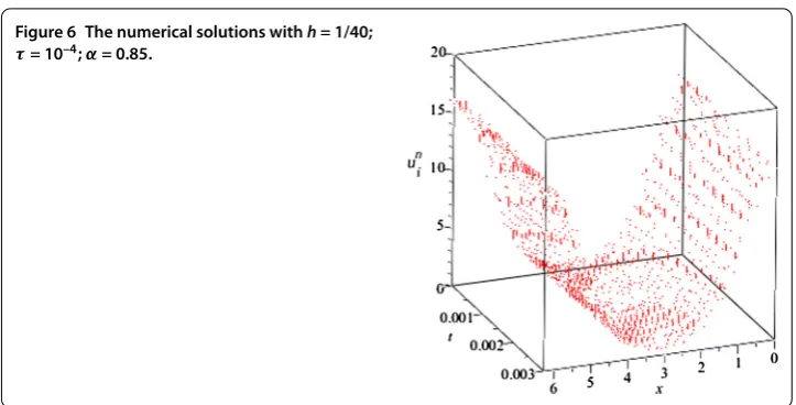
Figure 6 The numerical solutions withh= 1/40;

τ= 10–4;α= 0.85.

From Figures - we can see that the numerical solutions can well approximate the exact solutions with small errors, and the results in Tables - show that the convergence order in spatial direction is about of fourth order, which is in accordance with the theoretical analysis.

6 Conclusions

In this paper, we have developed a unconditionally stable finite difference scheme with spatial fourth-order accuracy for a class of time fractional parabolic equations with vari-able coefficient and proved the unique solvability, stability, and convergence of it by use of the Fourier analysis method. Numerical experiments for supporting the theoretical anal-ysis results were carried out. It is worth noting that for fractional differential equations with periodic boundary conditions, higher-order difference schemes can be also devel-oped, provided that the approximating orders in Lemma  increase.

Competing interests

The authors declare that they have no competing interests.

Authors’ contributions

QF carried out the main part of this article. Both authors read and approved the ﬁnal manuscript.

Author details

1_{School of Science, Shandong University of Technology, Zhangzhou Road 12, Zibo, Shandong 255049, China.}2_{School of} Mathematical Sciences, Qufu Normal University, Qufu, Shandong 273165, China.

Acknowledgements

This work was partially supported by Natural Science Foundation of China (11671227), Natural Science Foundation of Shandong Province (China) (ZR2013AQ009), and the development supporting plan for young teachers in Shandong University of Technology.

Received: 18 August 2016 Accepted: 22 November 2016 References

1. Kilbas, A, Srivastava, H, Trujillo, J: Theory and Applications of Fractional Diﬀerential Equations. Elsevier, Boston (2006) 2. Chen, C, Liu, F, Turner, I, Anh, V: Numerical simulation for the variable-order Galilei invariant advection diﬀusion

equation with a nonlinear source term. Appl. Math. Comput.217, 5729-5742 (2011)

3. Liu, F, Zhuang, P, Anh, V, Turner, I, Burrage, K: Stability and convergence of the diﬀerence methods for the space-time fractional advection-diﬀusion equation. Appl. Math. Comput.191, 12-20 (2007)

4. Chen, S, Liu, F: ADI-Euler and extrapolation methods for the two-dimensional fractional advection-dispersion equation. J. Appl. Math. Comput.26, 295-311 (2008)

(14)

6. Zhang, H, Liu, F, Phanikumar, MS, Meerschaert, MM: A novel numerical method for the time variable fractional order mobile-immobile advection-dispersion model. Comput. Math. Appl.66, 693-701 (2013)

7. Mohebbi, A, Abbaszadeh, M: Compact ﬁnite diﬀerence scheme for the solution of time fractional advection-dispersion equation. Numer. Algorithms63, 431-452 (2013)

8. Cui, M: A high-order compact exponential scheme for the fractional convection-diﬀusion equation. J. Comput. Appl. Math.255, 404-416 (2014)

9. Ji, C, Sun, Z: A high-order compact finite difference scheme for the fractional sub-diffusion equation. J. Sci. Comput. 64, 959-985 (2015)

10. Cui, M: Compact alternating direction implicit method for two-dimensional time fractional diﬀusion equation. J. Comput. Phys.231, 2621-2633 (2012)

11. Yuste, SB, Acedo, L: An explicit finite difference method and a new von Neumann-type stability analysis for fractional diffusion equations. SIAM J. Numer. Anal.42, 1862-1874 (2005)

12. Langlands, TAM, Henry, BI: The accuracy and stability of an implicit solution method for the fractional diﬀusion equation. J. Comput. Phys.205, 719-736 (2005)

13. Alikhanov, AA: A new diﬀerence scheme for the time fractional diﬀusion equation. J. Comput. Phys.280, 424-438 (2015)

14. Gao, G, Sun, Z: A compact finite difference scheme for the fractional sub-diffusion equations. J. Comput. Phys.230, 586-595 (2011)

15. Zhang, Y, Sun, Z, Wu, H: Error estimates of Crank-Nicolson-type diﬀerence schemes for the subdiﬀusion equation. SIAM J. Numer. Anal.49, 2302-2322 (2011)

16. Zhao, X, Xu, Q: Efficient numerical schemes for fractional sub-diffusion equation with the spatially variable coefficient. Appl. Math. Model.38, 3848-3859 (2014)

17. Vong, S, Lyu, P, Wang, Z: A compact difference scheme for fractional sub-diffusion equations with the spatially variable coefficient under Neumann boundary conditions. J. Sci. Comput.66, 725-739 (2016)

18. Wang, H, Yang, D, Zhu, S: A Petrov-Galerkin finite element method for variable-coefficient fractional diffusion equations. Comput. Methods Appl. Mech. Eng.290, 45-56 (2015)

19. Chen, S, Liu, F, Jiang, X, Turner, I, Anh, V: A fast semi-implicit difference method for a nonlinear two-sided space-fractional diffusion equation with variable diffusivity coefficients. Appl. Math. Comput.257, 591-601 (2014) 20. Wang, YM: A compact finite difference method for a class of time fractional convection-diffusion-wave equations.

Numer. Algorithms70, 625-651 (2015)