R E S E A R C H
Open Access
Periodic solution and control optimization
of a prey-predator model with two types of
harvesting
Jianmei Wang
1, Huidong Cheng
1*, Hongxia Liu
1,2and Yanhui Wang
1,2*Correspondence:
[email protected] 1College of Mathematics and
Systems Science, Shandong University of Science and Technology, Qingdao, China Full list of author information is available at the end of the article
Abstract
In this work, a prey-predator model with both state-dependent impulsive harvesting and constant rate harvesting is investigated, where the replenishment rate of prey and the harvesting rate are linearly related with the selected threshold. By first using the successor function method and differential equation geometry theory, the existence, uniqueness and asymptotic stability of the order-1 periodic solution are discussed. And then numerical simulations with an example are given to illustrate the feasibility of the theorem-related results. Moreover, in order to increase the total profit, the optimization strategy is presented and the optimal threshold is obtained.
MSC: 34C25; 34D20; 92B05; 34A37
Keywords: prey-predator model; state-dependent impulse; order-1 periodic solution; optimization; stability
1 Introduction
Fishery is the natural source and basis of fishery production, and it is also one of the im-portant food sources for human beings. If fishery resources are used properly, it can adapt to the natural regeneration ability of the resource and maintain the optimum sustainable yield. If people harvest fish unrestricted, it will lead to the extinction of the species [1–4]. Therefore, looking for a reasonable harvest strategy to ensure the sustainable development of fishery resources has become the focus of research.
In the past few decades, various harvest strategies have been proposed and implemented in fishing industry. In general, if a species is harvested frequently and regularly, we can adopt the strategy with constant rate harvesting [5–8]. And due to the seasonal and eco-nomic reasons, periodic harvesting is an effective harvesting strategy for the infrequent harvesting. This periodic harvesting can be described by impulsive differential equations [9–16]. There are some papers studying the effects of periodic impulse harvesting strat-egy to the species resource. For example, Peiet al.[17] proposed a continuous impulsive harvesting strategy for a prey-predator system with stage structure and time delay, and analysed the global attractivity of extinction periodic solution of the mature predator. Jiao et al.[18] considered a periodic impulsive harvesting prey-predator system with prey hi-bernation, and they obtained the conditions of the global asymptotic stability criterion for the predator-extinction boundary and the permanent conditions. However, these two
methods of harvesting are carried out without knowing the number of species, which can lead to overexploitation and even depletion of resources.
Recently, state-dependent impulse feedback control has attracted the attention of many scholars [19–23], a novel strategy based on state-dependent impulse feedback control is proposed and applied in the harvest [24–27] and pest management [28–33]. The proce-dure goes like this: when the number of species reaches a specific requirement, the har-vesting strategy is implemented, otherwise the harhar-vesting behavior is suppressed. Some other related studies can be found in [34–39] and the references therein.
Brauer and Soudack [5] considered the following prey-predator system with constant rate harvest for predator:
and analyzed the asymptotically stable interval of the system under different cases, where f1(x,y),f2(x,y), respectively, are the average growth rate ofxandy. After further research
the prey fish at ratep∈(0, 1) while harvesting the predator fish. The control parame-tersp(x),τ(x) andq(x) are continuous functions defined on [hmin,hmax] (see [42]), where hmin andhmax are, respectively, the minimum value and maximum value of the thresh-old which satisfy 0 <hmin≤h≤hmax<K1––pτmin
min. Furthermore,p(hmax) =pmin,p(hmin) =pmax,
τ(hmax) =τmin,τ(hmin) =τmax,q(hmax) =qminandq(hmin) =qmax. Denoteph=p(h),τh=τ(h) andqh=q(h).
The main contents of this work are organized as follows. In Section 2, some main defi-nitions and lemmas are provided. In Section 3, the existence, uniqueness and asymptotic stability of the order-1 periodic solution of system (2) are mainly discussed under some conditions. The theoretical results are then verified by numerical simulations, and the op-timization problem is presented and solved for obtaining the maximum harvesting profits in Section 4. This work ends with a conclusion.
2 Preliminaries
Definition 2.1([43]) Consider the general differential system with state-dependent im-pulse
The dynamic system constituted by the solution mappings of system (4) is called a semi-continuous dynamic system, which is denoted as (,g,I,M). Let the initial pointA∈= R2
+\M, and the functionI is a continuous impulse mapping that satisfiesI:M→N.
MandNare, respectively, the impulsive set and the phase set which represent the curves or straight lines in the planeR2+. system (4) with periodT.
Definition 2.3([45]) Assume =g(A,t) is an order-1 periodic solution of system (4). The order-1 periodic solution is orbitally asymptotically stable if for anyε> 0, there must existδ> 0 andt0≥0, such that, for any pointA1∈U(A,δ)∩Nandt>t0, we have
ρ(g(A1,t),) <ε.
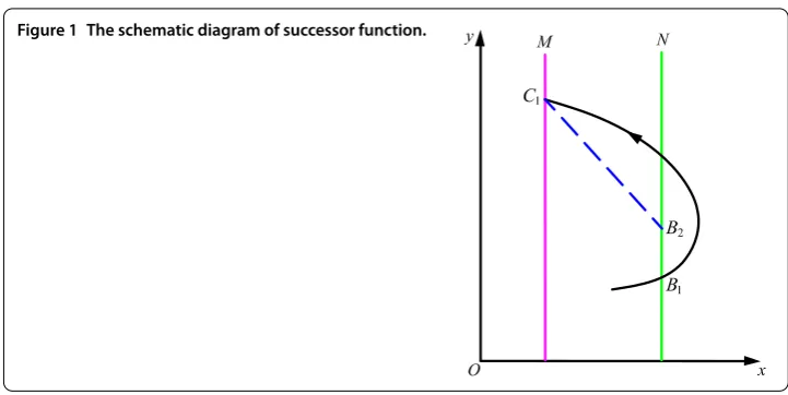
Definition 2.4 ([46]) Assuming that the impulse setMand the phase set N are both straight lines; see Figure 1. For any pointB1∈N, we have(B1,t) =C1∈M,I(C1) =B2∈
N, thenB2is defined as the successor point ofB1, andg(B1) =yB2–yB1 is defined as the
Figure 1 The schematic diagram of successor function.
Lemma 2.1([47]) Successor function g(B1)is continuous.
Lemma 2.2([48]) In system(4),if there exist A∈N,B∈N satisfying successor function
g(A)g(B) < 0,then there must exist a point S(S∈N)satisfying S between point A and point B such that g(S) = 0,thus system(4)has an order-1periodic solution.
3 Dynamical analysis of system (2)
The dynamical properties of the order-1 periodic solution of system (2) are mainly inves-tigated in this section. Before these discussions, we firstly analyze the qualitative charac-teristics of system (2) without control, and the conditions that system (2) without control has no closed orbit are discussed.
3.1 Qualitative analysis of system (2) without control
Consider the continuous system of system (2) without control as follows:
⎧ ⎨ ⎩
x(t) =ax(t)(1 –xK(t)) –bx(t)y(t) =P(x,y),
y(t) =y(t)(λbx(t) –d) –H=Q(x,y). (5)
By setting
⎧ ⎨ ⎩
ax(t)(1 –xK(t)) –bx(t)y(t) = 0,
y(t)(λbx(t) –d) –H= 0, (6)
we have
aλ K x
2– aλ+ad
bK
x+ad
b +H= 0.
Let
= aλ+ ad bK
2
– 4aλ K
ad b +H
thus we find that if the condition
holds, then the system (5) has two positive equilibria which are denoted asE1(xE1,yE1) and
E2(xE2,yE2), where
Next, the stability of these two equilibria are discussed. The Jacobian matrix at equilib-riumEi,i= 1, 2, is but not saddle-type positive equilibrium, andE2(xE2,yE2) is a saddle.
On the other hand, if the condition
(H2) : λb–
a K < 0
holds, thenTr(J(E1)) < 0, which meansE1(xE1,yE1) is a locally asymptotically stable focus or node.
In the following, let Dulac functionB=x–1, then we get
D=∂(BP)
According to the Bendixson-Dulac theorem, the closed orbit of system (5) does not exist in the planeR2
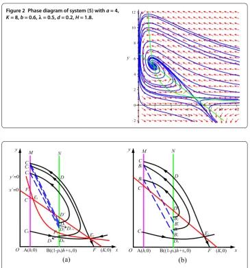
Figure 2 Phase diagram of system (5) witha= 4,
K= 8,b= 0.6,λ= 0.5,d= 0.2,H= 1.8.
Figure 3 The existence and uniqueness of the order-1 periodic solution of system (2) in Case I. (a)The existence of the periodic solution.(b)The uniqueness of the periodic solution.
Theorem 3.1 System(5)has two positive equilibrium:a locally asymptotically stable focus or node E1(xE1,yE1)and a saddle E2(xE2,yE2),and there is no closed trajectory in the plane
R2
+if the conditions(H1)and(H2)hold(see Figure2).
3.2 Existence, uniqueness and stability of order-1 periodic solution
According to ecological significance, system (2) should satisfy 0 <h< (1 –ph)h+τh<K. By the discussion in the previous subsection, we have thex-isolinex= 0 intersectsy-isoline y= 0 at pointE1(xE1,yE1) and pointE2(xE2,yE2) (see Figure 3(a)). For notation simplicity,
let thex-axis intersect the linex=h(impulse setM) at pointA(h, 0) and intersect the line x= (1 –ph)h+τh(phase setN) at pointB((1 –ph)h+τh, 0), thex-isolinex= 0 intersect the linesx=handx= (1 –ph)h+τhat pointsCandD, respectively, they-isoliney= 0 intersect the linesx=handx= (1 –ph)h+τh, respectively, at pointsF1andF2.C,DandF
are, respectively, the intersections between the stable flow ofE2(xE2,yE2) and the linex=h,
the linex= (1 –ph)h+τh,x-axis.C0andD0are, respectively, the intersections between
Theorem 3.2 System(2)exists a unique order-1periodic solution if the conditions(H1),
(H2)and0 <h< (1 –ph)h+τh<K hold.
Proof For different thresholdh, let us consider three cases as follows. Case I. 0 <h<xE1< (1 –ph)h+τh<xE2.
There exists a thresholdh∈(0,xE1) such thatqh∈[qmin,qmax], due to impulsive effects, pointCjumps to a pointD1∈D0D⊂N, thenyD0 <yD1= (1 –qh)yC<yD. Besides, the
orbit of system (2) starting from pointD1must pass through a pointC1∈M, then jumps
back to a pointD2∈N. Because distinct orbits are disjoint, thenyC<yC1<yCandyD2=
(1 –qh)yC1 < (1 –qh)yC=yD1, thus the successor function of pointD1 isg(D1) =yD2 – yD1< 0.
Moreover, another point D ∈D0Dis selected and satisfies yD =yD0 + ( > 0 suf-ficiently small). There must be an orbit starting from point D and passing through
pointC ∈M, and pointC is next to pointC, due to impulsive effects, pointC jumps
to a point D+1 ∈N. Because distinct orbits are disjoint, we knowyC1 <yC <yC and yD<yD2= (1 –qh)yC1< (1 –qh)yC=yD+1. Then we haveg(D) =yD+1–yD> 0.
We can easily get g(D1)g(D) < 0, there is a point S ∈DD1 such that f(S) = 0 by
Lemma 2.2,i.e.the order-1 periodic solution is existent.
In the following, the uniqueness of the order-1 periodic solution is proved. Arbitrarily select two pointsB1andB2in the linex= (1 –p)hh+τhwhich meetyD0<yB1<yB2 <yD (see Figure 3(b)). The orbits of system (2) starting from pointsB1andB2, respectively,
reach pointsB–
1 ∈MandB–2 ∈M, and satisfyyC<yB–2 <yB–1 <yC, then jump back to the linex= (1 –ph)h+τhatB+1andB+2 by impulsive effects, respectively. Then the successor
functions of pointsB1andB2must satisfy
g(B2) –g(B1) = (yB2+–yB2) – (yB+1 –yB1) = (yB+
2–yB+1) + (yB1–yB2) < 0,
which illustrates the successor functiongin the segmentD0Dis monotonically
decreas-ing, thus there is only one pointS∈D0Dthat makesg(S) = 0.
For any pointS1∈DD, the orbit of system (2) starting from pointS1intersects a point in
the linex=hwhich is denoted asS1–, then jumps to a pointS1+∈Nafter impulsive effects. Because distinct orbits are disjoint, thenyC<yS–
1 <yCandyS+1 = (1 –qh)yS1–< (1 –qh)yC= yD1 <yS1, thus we getg(S1) =yS+1 –yS1 < 0, which says there is no order-1 periodic orbit
passing through pointS1∈DD. In addition, for any pointS2∈BD0, the orbit starting
from pointS2 eventually passes through the liney= 0 and unaffected by any impulse,
namely, there is no order-1 periodic orbit passing through pointS2.
Case II.xE1≤h< (1 –ph)h+τh≤xE2.
The following steps are similar to the Case I and omitted thereby (see Figure 4). Case III.xE1<h<xE2< (1 –ph)h+τh<K.
For this subcase, the stable flow ofE2intersects the linex= (1 –p)hh+τhat pointG1, and
the unstable flow ofE2intersects the linex= (1 –p)hhat pointH1. We can select a point
G satisfyingyG=yG1+, there must exist an orbit starting from pointG and passing through pointH∈M, and pointH is next to pointH1. By impulsive effects, pointH
Figure 4 The existence of the order-1 periodic solution of system (2) in Case II.
Figure 5 The existence and uniqueness of the order-1 periodic solution of system (2) in Case III. (a)The existence of the periodic solution.(b)The uniqueness of the periodic solution.
Furthermore, we can select another orbit that is far from the stable flow and unstable flow ofE2which passes through pointG2∈N, and reaches pointH2∈M, then jumps
back to the linex= (1 –ph)h+τhat pointG3, and pointG3is below pointG2, theng(G2) =
yG3–yG2< 0.
We can easily get g(G)g(G2) < 0. Then there is a pointS∈GG2 such thatg(S) = 0,
namely, the order-1 periodic solution is existent (see Figure 5(a)).
Next, we prove the uniqueness of the periodic solution. From Figure 5(b), arbitrarily select two pointsB3∈NandB4∈Nwhich meetyG1<yB3<yB4<yG2. The orbits of system
(2) starting from pointsB3andB4respectively reach at pointsB3–∈MandB–4∈M, and
satisfyyH1<yB–
3 <yB–4 <yH2, then jump back to the linex= (1 –ph)h+τhatB
+
3andB+4due
successor functions of pointsB3andB4must satisfy
g(B4) –g(B3) = (yB+4–yB4) – (yB+3 –yB3) < 0,
which illustrates, in the segmentG1G2, the successor functionf is monotonically
decreas-ing, thus there is only one pointS∈G1G2that makesg(S) = 0.
For any pointS3∈G1B, the orbit starting from pointS3eventually passes through the
liney= 0 and unaffected by any impulse, namely, there is no order-1 periodic orbit passing
through pointS3∈G1B.
In this paper, we assume that the order-1 periodic solution of system (2) isSS–S, where
S∈N andS–∈M. Next we prove the stability of the periodic solutionSS–S. Since the
methods used in the above three cases are similar, we only prove Case II.
Theorem 3.3 The periodic solutionSS–S is orbitally asymptotically stable if xE1<h< (1 –
ph)h+τh<xE2andab(1 –qh)(1 –Kh)≥λb[(1–phH)h+τh]–d hold under Theorem3.2.
Proof From Figure 4 we can seeyF2=λb[(1–pH
h)h+τh]–d>yD0. Besides, byyC=
a b(1 –
h K) and a
b(1 –qh)(1 – h K)≥
H
λb[(1–ph)h+τh]–d, it is easy to know (1 –qh)yC ≥yF2 >yD0, then, for any
pointS4∈CC, we get (1 –qh)yS4≥(1 –qh)yC≥yF2>yD0. We know the periodic solution
SS–Sis unique, whereS∈D
0D1. From Figure 6 we can see the orbit of system (2) starting
fromD1intersects the linex=hat pointC1, then jumps bake to the linex= (1 –ph)h+τh at pointD2due to impulsive effects. Because distinct orbits are disjoint, we haveyC <
yC1<yS– andyD0<yD2 <yS. The orbit starting fromD2intersects the linex=hat point C2, then jumps bake to the linex= (1 –ph)h+τhat pointD3after impulsive effects, where
yS–<yC2<yCandyS<yD3<yD1.
Repeat the above process, the orbit starting from pointD0will be subjected to impulsive
effects infinitely times. Denote the successor point of pointDiasDi+1,i= 0, 1, 2, . . . , then
we get
yD0<yD2<yD4<· · ·<yD2i<yD2(i+1)<· · ·<yS
and
yD1>yD3>yD5>· · ·>yD2i+1>yD2(i+1)+1>· · ·>yS.
Therefore, the sequence{D2i}is monotonically increasing and the sequence{D2i+1}is
monotonically decreasing. Besides,
yD2i→yS, asi→ ∞,
and
yD2i+1→yS, asi→ ∞.
We select any pointP0∈D0D1and letyD0<yP0<yS(otherwise,yD1>yP0>yS, the proofs
are similar), then there must be a positive integer k0 which satisfyyD2k0 <yP0 <yD2(k0+1).
The orbit starting from pointP0will be affected by impulse infinitely times. Affected by
thejth impulse, the corresponding phase point is denoted asPj,j= 1, 2, . . . , then, for any n, we getyD2(k0+n) <yP2n<yD2(k0+n+1) andyD2(k0+n+1)<yP2n+1<yD2(k0+n)+1,n= 0, 1, 2, . . . , thus
{yP2n}is monotonically increasing, and{yP2n+1}is monotonically decreasing, and
yD2n→yS, asn→ ∞,
and
yD2n+1→yS, asn→ ∞.
Therefore, all the successor points in the segmentDD0are attracted to pointSafter the
corresponding impulsive effect, then the periodic solutionSS–Sis orbitally asymptotically
stable. That completes the proof.
4 Simulations and optimization 4.1 Numerical simulations
A specific model is given in this subsection to verify the effectiveness of our conclusions. Leta= 4,K= 8,b= 0.6,λ= 0.5,d= 0.2,H= 1.8,hmax= 6,hmin= 1.3,pmax= 0.01,pmin= 0.001,τmax= 1.4,τmin= 1.27,qmax= 0.7,qmin= 0.52. By calculation, the equilibrium points of system (5) areE1(1.8344, 5.1380) andE2(6.8322, 0.9731). These parameter values are
substituted into system (2), then we find
⎧ ⎪ ⎪ ⎪ ⎪ ⎪ ⎪ ⎨ ⎪ ⎪ ⎪ ⎪ ⎪ ⎪ ⎩
x(t) = 4x(t)(1 –x(8t)) – 0.6x(t)y(t), y(t) =y(t)(0.3x(t) – 0.2) – 1.8,
⎫ ⎬ ⎭ x>h,
x(t) = –p(x)x(t) +τ(x), y(t) = –q(x)y(t),
⎫ ⎬ ⎭ x=h.
(7)
Leth= 1.5 satisfy the condition 0 <h<xE1, we select the orbit starting from (4, 4). A di-rected calculation yields p1.5= 0.0096,τ1.5= 1.3945 andq1.5= 0.6923 which satisfy the
Figure 7 Numerical simulations in the case 0 <h<xE1< (1 –ph)h+τh<xE2. (a)Phase portrait of prey
fish density and predator fish density onh= 1.5.(b)Time series of prey fish density.(c)Time series of predator fish density.
Figure 8 Numerical simulations in the casexE1<h< (1 –ph)h+τh<xE2. (a)Phase portrait of prey fish
density and predator fish density onh= 4.(b)Time series of prey fish density.(c)Time series of predator fish density.
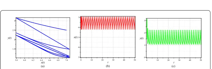
Figure 9 Numerical simulations in casexE1<h<xE2< (1 –ph)h+τh<K. (a)Phase portrait of prey fish
density and predator fish density onh= 5.8.(b)Time series of prey fish density.(c)Time series of predator fish density.
Furthermore, we obtain the period of order-1 periodic solution isT= 3.5667 by observ-ing from Figure 7(b).
The phase portrait and time series of prey fish density and predator fish density are shown in Figure 8 for h= 4 with the initial value (5, 3.5), by calculation we obtain p4=
0.0048,τ4= 1.3253 andq4= 0.5966 which satisfy the conditionxE1<h< (1 –ph)h+τh< xE2. Then system (7) exists a unique and orbitally asymptotically stable order-1 periodic solution, and the period isT= 1.4625; see Figures 8(a), 8(b) and 8(c).
For the case ofxE1 <h<xE2 < (1 –ph)h+τh<K, for exampleh= 5.8 and the orbit of system (7) starting from (7, 2.5), by calculation, we getp5.8= 0.0014,τ5.8= 1.2755 andq5.8=
4.2 Determination of optimal thresholdh
The practical significance of studying the order-1 periodic solution is that it provides the possibility to determine the replenishment rate of prey fish and the harvesting rate of predator fish, which makes the impulsive control to be not a real-time monitoring of fish-eries, but rather a periodic one. In order to maintain the ecological balance of fishfish-eries, further determine the optimal replenishment rate of prey fish and the optimal harvesting rate of predator fish, and make sure the harvest period is shortest and the profit is highest, we consider the following optimization problem to find the optimal threshold.
Letl1 denote the unit cost of prey fish replenished including the cost of dealing with
fisheries environment,l2be the unit income of predator fish. Our objective is to minimize
costs and maximize profits in this process. DenoteF as the total profit in one period of system (7), which is a function of replenishment rate of prey fishτh and the harvesting rate of predator fishqh. SinceH is constant and has no effect on the change in profits, then we no longer consider it and haveF(h) =l2qh–l1τh. Thus, the optimization model is formulated as
maxF(h)
T(h)
s.t. hmin≤h≤hmax
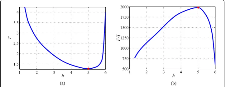
The optimization problem is solved to yield the optimal thresholdh∗, which results in the optimal replenishment rate of prey fishτ∗=ph∗, the optimal harvesting rate of preda-tor fishq∗=qh∗, and the optimal impulse periodT∗=T(τ∗,q∗). The impulse periodT varies with the thresholdh, as shown in Figure 10(a), and the relationship between the profit per unit timeF/T and the thresholdhis presented in Figure 10(b), wherel1= 200,
l2= 5000,i.e.,l2/l1= 25. From Figure 10, the optimal threshold ish∗= 5, then the optimal
replenishment rate of prey fishτ∗= 1.2977, the optimal harvesting rate of predator fish q∗= 0.5583, and the optimal impulse period isT∗= 1.2767.
5 Conclusion
This work presents a prey-predator system with both state-dependent impulsive harvest-ing and constant rate harvestharvest-ing, where the harvestharvest-ing frequency of constant harvestharvest-ing
is more frequent than that of impulse harvesting. Moreover, the combination of these two harvesting methods is more practical which provides higher commercial value and avoids the exhaustion of resources. Meanwhile, the existence, uniqueness and stability of the order-1 periodic solution are proved by using the method of successor functions and differential equation geometry theory. Numerical simulations with a specific example are given to verify feasibility of the impulsive strategy. Furthermore, to maximize economic benefit, we provide an optimization strategy for the pisciculture and obtain the optimal threshold. However, the optimization results have some deviations which need to be fur-ther improved.
Acknowledgements
The paper is supported in part by the National Natural Science Foundation of China (No. 11371230, 11501331), in part by Shandong Provincial Natural Science Foundation, China (No. S2015SF002), in part by SDUST Research Fund
(2014TDJH102), and in part by Joint Innovative Center for Safe and Effective Mining Technology and Equipment of Coal Resources, Shandong Province of China.
Competing interests
The authors claim that they have no competing interests.
Authors’ contributions
All authors read and approved the final manuscript.
Author details
1College of Mathematics and Systems Science, Shandong University of Science and Technology, Qingdao, China.2State
Key Laboratory of Mining Disaster Prevention and Control Co-founded by Shandong Province and the Ministry of Science and Technology, Shandong University of Science and Technology, Qingdao, China.
Publisher’s Note
Springer Nature remains neutral with regard to jurisdictional claims in published maps and institutional affiliations.
Received: 27 October 2017 Accepted: 18 January 2018
References
1. Pal, D, Mahapatra, GS: A bioeconomic modeling of two-prey and one-predator fishery model with optimal harvesting policy through hybridization approach. Appl. Math. Comput.242, 748-763 (2014)
2. Liu, G, Wang, X, Meng, X, Gao, S: Extinction and persistence in mean of a novel delay impulsive stochastic infected predator-prey system with jumps. Complexity2017(3), Article ID 1950970 (2017)
3. Liu, L, Meng, X: Optimal harvesting control and dynamics of two-species stochastic model with delays. Adv. Differ. Equ.2017(1), 18 (2017)
4. Bian, F, Zhao, W, Song, Y, Yue, R: Dynamical analysis of a class of prey-predator model with Beddington-Deangelis functional response, stochastic perturbation, and impulsive toxicant input. Complexity2017, Article ID 3742197 (2017)
5. Brauer, F, Soudack, AC: Stability regions in predator-prey systems with constant-rate prey harvesting. J. Math. Biol.
8(1), 55-71 (1979)
6. Martin, A, Ruan, S: Predator-prey models with delay and prey harvesting. J. Math. Biol.43(3), 247-267 (2001) 7. Xiao, D, Li, W, Han, M: Dynamics in a ratio-dependent predator-prey model with predator harvesting. J. Math. Anal.
Appl.324(1), 14-29 (2006)
8. Chen, L, Chen, F: Global analysis of a harvested predator-prey model incorporating a constant prey refuge. Int. J. Biomath.3(02), 205-223 (2010)
9. Zhang, T, Ma, W, Meng, X: Global dynamics of a delayed chemostat model with harvest by impulsive flocculant input. Adv. Differ. Equ.2017(1), 115 (2017)
10. Wang, Y, Jiang, W, Wang, H: Stability and global Hopf bifurcation in toxic phytoplankton-zooplankton model with delay and selective harvesting. Nonlinear Dyn.73(1), 881-896 (2013)
11. Meng, X, Wang, L, Zhang, T: Global dynamics analysis of a nonlinear impulsive stochastic chemostat system in a polluted environment. J. Appl. Anal. Comput.6(3), 865-875 (2016)
12. Zhang, T, Meng, X, Song, Y: The dynamics of a high-dimensional delayed pest management model with impulsive pesticide input and harvesting prey at different fixed moments. Nonlinear Dyn.64(1), 1-12 (2011)
13. Jiang, Z, Wang, L: Global Hopf bifurcation for a predator-prey system with three delays. Int. J. Bifurc. Chaos27(07), 1750108 (2017)
14. Zhang, S, Meng, X, Feng, T, Zhang, T: Dynamics analysis and numerical simulations of a stochastic non-autonomous predator-prey system with impulsive effects. Nonlinear Anal. Hybrid Syst.26, 19-37 (2017)
15. Meng, X, Zhang, L: Evolutionary dynamics in a Lotka-Volterra competition model with impulsive periodic disturbance. Math. Methods Appl. Sci.39(2), 177-188 (2016)
17. Pei, Y, Li, C, Chen, L: Continuous and impulsive harvesting strategies in a stage-structured predator-prey model with time delay. Math. Comput. Simul.79(10), 2994-3008 (2009)
18. Jiao, J, Cai, S, Li, L: Dynamics of a periodic switched predator-prey system with impulsive harvesting and hibernation of prey population. J. Franklin Inst.353(15), 3818-3834 (2016)
19. Huang, C, Meng, Y, Cao, J, Alsaedi, A, Alsaadi, FE: New bifurcation results for fractional BAM neural network with leakage delay. Chaos Solitons Fractals100, 31-44 (2017)
20. Huang, C, Cao, J, Xiao, M, Alsaedi, A, Hayat, T: Effects of time delays on stability and Hopf bifurcation in a fractional ring-structured network with arbitrary neurons. Commun. Nonlinear Sci. Numer. Simul.57, 1-13 (2018) 21. Huang, C, Cao, J, Xiao, M, Alsaedi, A, Hayat, T: Bifurcations in a delayed fractional complex-valued neural network.
Appl. Math. Comput.292, 210-227 (2017)
22. Huang, C, Cao, J, Xiao, M, Alsaedi, A, Alsaadi, FE: Controlling bifurcation in a delayed fractional predator-prey system with incommensurate orders. Appl. Math. Comput.293, 293-310 (2017)
23. Zhang, T, Ma, W, Meng, X, Zhang, T: Periodic solution of a prey-predator model with nonlinear state feedback control. Appl. Math. Comput.266, 95-107 (2015)
24. Jiao, J, Chen, L, Long, W: Pulse fishing policy for a stage-structured model with state-dependent harvesting. J. Biol. Syst.15(03), 409-416 (2008)
25. Nie, L, Teng, Z, Hu, L, Peng, J: The dynamics of a Lotka-Volterra predator-prey model with state dependent impulsive harvest for predator. Biosystems98(2), 67-72 (2009)
26. Huang, M, Song, X: Periodic solutions and homoclinic bifurcations of two predator-prey systems with nonmonotonic functional response and impulsive harvesting. J. Appl. Math.2014, Article ID 803764 (2014)
27. Wei, C, Chen, L: Periodic solution and heteroclinic bifurcation in a predator-prey system with Allee effect and impulsive harvesting. Nonlinear Dyn.76(2), 1109-1117 (2014)
28. Yang, J, Tang, S: Holling type II predator-prey model with nonlinear pulse as state-dependent feedback control. J. Comput. Appl. Math.291, 225-241 (2016)
29. Cheng, H, Zhang, T, Wang, F: Existence and attractiveness of order one periodic solution of a Holling I predator-prey model. Abstr. Appl. Anal.2012, Article ID 126018 (2012)
30. Zhang, H, Georgescu, P, Zhang, L: Periodic patterns and Pareto efficiency of state dependent impulsive controls regulating interactions between wild and transgenic mosquito populations. Commun. Nonlinear Sci. Numer. Simul.
31(1), 83-107 (2016)
31. Cheng, H, Wang, F, Zhang, T: Multi-state dependent impulsive control for pest management. J. Appl. Math.2012, Article ID 381503 (2012)
32. Tian, Y, Zhang, T, Sun, K: Dynamics analysis of a pest management prey-predator model by means of interval state monitoring and control. Nonlinear Anal. Hybrid Syst.23, 122-141 (2017)
33. Zhang, T, Meng, X, Liu, R, Zhang, T: Periodic solution of a pest management Gompertz model with impulsive state feedback control. Nonlinear Dyn.78(2), 921-938 (2014)
34. Miao, A, Zhang, J, Zhang, T, Pradeep, BGSA: Threshold dynamics of a stochastic SIR model with vertical transmission and vaccination. Comput. Math. Methods Med.2017, 4820183 (2017)
35. Miao, A, Wang, X, Zhang, T, Wang, W, Pradeep, BGSA: Dynamical analysis of a stochastic SIS epidemic model with nonlinear incidence rate and double epidemic hypothesis. Adv. Differ. Equ.2017, 226 (2017)
36. Zhao, W, Li, J, Meng, X: Dynamical analysis of SIR epidemic model with nonlinear pulse vaccination and lifelong immunity. Discrete Dyn. Nat. Soc.2015, Article ID 848623 (2015)
37. Leng, X, Feng, T, Meng, X: Stochastic inequalities and applications to dynamics analysis of a novel SIVS epidemic model with jumps. J. Inequal. Appl.2017, 138 (2017)
38. Lv, W, Wang, F: Adaptive tracking control for a class of uncertain nonlinear systems with infinite number of actuator failures using neural networks. Adv. Differ. Equ.2017(1), 374 (2017)
39. Lv, X, Wang, L, Meng, X: Global analysis of a new nonlinear stochastic differential competition system with impulsive effect. Adv. Differ. Equ.2017(1), 296 (2017)
40. Huang, M, Liu, S, Song, X, Chen, L: Periodic solutions and homoclinic bifurcation of a predator-prey system with two types of harvesting. Nonlinear Dyn.73, 815-826 (2013)
41. Xiao, Q, Dai, B, Xu, B, Bao, L: Homoclinic bifurcation for a general state-dependent Kolmogorov type predator-prey model with harvesting. Nonlinear Anal., Real World Appl.26, 263-273 (2015)
42. Sun, K, Zhang, T, Tian, Y: Theoretical study and control optimization of an integrated pest management predator-prey model with power growth rate. Math. Biosci.279, 13-26 (2016)
43. Chen, L: Pest control and geometric theory of semi-continuous dynamical system. J. Beihua Univ. Nat. Sci.12(1), 1-9 (2011)
44. Liu, B, Tian, Y, Kang, B: Dynamics on a Holling II predator-prey model with state-dependent impulsive control. Int. J. Biomath.5(03), 675 (2012)
45. Wang, J, Cheng, H, Meng, X, Pradeep, BSA: Geometrical analysis and control optimization of a predator-prey model with multi state-dependent impulse. Adv. Differ. Equ.2017(1), 252 (2017)
46. Zhao, W, Liu, Y, Zhang, T, Meng, X: Geometric analysis of an integrated pest management model including two state impulses. Abstr. Appl. Anal.2014(1), 91506 (2014)
47. Cheng, H, Wang, F, Zhang, T: Multi-state dependent impulsive control for Holling I predator-prey model. Discrete Dyn. Nat. Soc.2012(12), 30-44 (2012)