Assessment of PSO Algorithm For Multi machine System Using STATCOM Device

© 2015, IRJET.NET- All Rights Reserved

Page 2262

Assessment of PSO Algorithm For Multi-machine System

Using STATCOM Device

A.Sagarika

, T.R.Jyothsna

PG Student [Power Systems], Dept. of EEE, Andhra University, Visakhapatnam, India

Professor, Dept. of EEE, Andhra University, Visakhapatnam,

India

---***---Abstract

Transient stability of power systems becomes a major factor in planning and day-to-day operations and there is a need for fast on-line solution of transient stability to predict any possible loss of synchronism and to take the necessary measures to restore stability. Recently various controller devices are designed to damp these oscillations and to improve the system stability, which are found in modern power systems, but static synchronous compensator (STATCOM) still remains an attractive solution. These STATCOM are local controllers on the generators. Thus local controllers are used to mitigate system oscillation modes. In multi machine system with several poorly damped modes of oscillations, several controllers have to be used and the problem of synthesis of STATCOM parameters becomes relatively complicated. Population based optimization techniques have been applied for STATCOM design. Studies have revealed that these optimization techniques have improved the system stability. A population based algorithm called Particle Swarm Optimization (PSO) has been proposed in this thesis for optimal tuning of the static synchronous series compensator (STATCOM) for a single machine infinite bus (SMIB) system. Recent studies in artificial intelligence demonstrated that the Particle Swarm optimization technique is a powerful intelligent tool for complicated stability problems. This algorithm is based on behavior of swarm intelligence occur in nature like flocking birds tend to form swarming patterns. The STATCOM parameters of an SMIB system and 3 machine system are tuned to improve small signal stability and large signal stability. It is relevant from the results that the proposed PSO algorithm is superior to any conventional technique.

Key Words:

I

.INTRODUCTION

1.1

STATCOM previously known as STATCON or Static condenser is an advanced static var compensator (SVC)

using voltage source converters with capacitors connected on DC side. STATCOM resembles in many respects a rotating synchronous condenser used for voltage control and reactive power compensation. As compared to conventional SVC, STATCOM does not require expensive large inductors; moreover it can also operate as reactive power sink or source flexibility, which makes STATCOM more attractive. Because of its several advantages over conventional SVC, it is expected to play a major role in the optimum and secure operation of AC transmission system in future

A static synchronous generator operated without an external electric energy source as a series compensator whose output voltage is in quadrature with, and controllable independently of, the line current for the purpose of increasing or decreasing the overall reactive voltage drop across the line and thereby controlling the transmitted electric power. The SSSC may include transiently rated energy storage or energy absorbing devices to enhance the dynamic behavior of the power system by additional temporary active power compensation, to increase or decrease momentarily, the overall active (resistive) voltage drop across the line. II. Particle Swarm Optimization

Inspired by the flocking and schooling patterns of birds and fish, Particle Swarm Optimization (PSO) was invented by Russell Eberhart and James Kennedy in 1995. Originally, these two started out developing computer software simulations of birds flocking around food sources, then later realized how well their algorithms worked on optimization problems.

© 2015, IRJET.NET- All Rights Reserved

Page 2263

implement.The algorithm keeps track of three global variables:

Target value or condition Global best (gBest) value indicating which particle's data is currently closest to the Target

Stopping value indicating when the algorithm should stop if the Target isn't found

Each particle consists of:

1. Data representing a possible solution

2. A Velocity value indicating how much the Data can be changed

3. A personal best (pBest) value indicating the closest the particle's Data has ever come to the Target

The particles' data could be anything. In the flocking birds example above, the data would be the X, Y, Z coordinates of each bird. The individual coordinates of each bird would try to move closer to the coordinates of the bird which is closer to the food's coordinates (gBest). If the data is a pattern or sequence, then individual pieces of the data would be manipulated until the pattern matches the target pattern.

The velocity value is calculated according to how far an individual's data is from the target. The further it is, the larger the velocity value. In the birds example, the individuals furthest from the food would make an effort to keep up with the others by flying faster toward the gBest bird. If the data is a pattern or sequence, the velocity would describe how different the pattern is from the target, and thus, how much it needs to be changed to match the target.

Each particle's pBest value only indicates the closest the data has ever come to the target since the algorithm started.

The gBest value only changes when any particle's pBest value comes closer to the target than gBest. Through each iteration of the algorithm, gBest gradually moves closer and closer to the target until one of the particles reaches the target.

It's also common to see PSO algorithms using population topologies, or "neighbourhoods", which can be smaller, localized subsets of the global best value. These neighbourhoods can involve two or more particles which are predetermined to act together, or subsets of the search space that particles happen into during testing. The use of neighbourhoods often helps the algorithm to avoid getting stuck in local minima.

PSO shares many similarities with evolutionary computation techniques such as Genetic Algorithms (GA). The system is initialized with a population of random solutions and searches for optima by updating generations. However, unlike GA, PSO has no evolution operators such as crossover and mutation. In PSO, the potential solutions, called particles, fly through the problem space by following the current optimum particles.

Each particle keeps track of its coordinates in the problem space which are associated with the best solution (fitness) it has achieved so far. (The fitness value is also stored.) This value is called pbest. Another "best" value that is tracked by the particle swarm optimizer is the best value, obtained so far by any particle in the neighbours of the particle. This location is called lbest. When a particle takes all the population as its topological neighbours, the best value is a global best and is called gbest.

The particle swarm optimization concept consists of, at each time step, changing the velocity of (accelerating) each particle toward its pbest and lbest locations (local version of PSO). Acceleration is weighted by a random term, with separate random numbers being generated for acceleration toward pbest and lbest locations.

In past several years, PSO has been successfully applied in many research and application areas. It is demonstrated that PSO gets better results in a faster, cheaper way compared with other methods.

Due to these attractive characteristics, i.e. memory and cooperation, PSO is widely applied in many research area and real-world engineering fields as a powerful optimization tool.

In PSO, each single solution is a particle in the search space. Each individual in PSO flies in the search space with a velocity, which is dynamically adjusted according to the flying experience of its own and its companions. PSO is initialized with a group of random particles. Each particle is treated as a point in a D-dimensional space. The ith particle is represented as xi = (xi1, xi2, . . ., xiD). The best previous position of the ith particle that give the best fitness value is represented as pi = (pi1, pi2, . . ., piD). The best particle among all the particles in the population is represented by pg = (pg1, pg2, . . ., pgD). Velocity, the rate of the position change for particle i is represented as vi = (vi1, vi2, . . . , viD). In every iteration, each particle is updated by following the two best values. After finding the aforementioned two best values, the particle updates its velocity and positions according to the following equations:

viD(new)=viD(old) + c1 r1(piD − xiD) + c2 r2(pgD − xiD) (2.1)

xiD(new)=xiD(old)+viD(new) (2.2) where c1 and c2 are two positive constants named as

© 2015, IRJET.NET- All Rights Reserved

Page 2264

2.2 PARAMETER SELECTION

1. Range of the particles

The ranges of the particles depend on the problem to be optimized. One can specify different ranges for different dimension of the particles

2. Maximum velocity vmax

The maximum velocity vmax determines the maximum change one particle can take during one iteration. Usually, the range of the particle is set as vmax. In this work, a vmax = 4 is chosen for each particle as this gives better optimal results.

3. The inertia parameter

The inertia parameter is introduced by Shi and

Eberhart

and provides improved performance in a

number of applications. It has control over the

impact of the previous history of velocities on

current velocity and influences the balance between

global and local exploration abilities of the

It is suggested to range w in a decreasing way from 1.4 to 0 adaptively. In this work, a constant value of the inertia parameter w = 0.75 is chosen as it facilitates reaching a better optimal value in lesser number of iterations. 4. The parameters c1 and c2

The acceleration constants c1 and c2 indicate the stochastic acceleration terms which pull each particle towards the best position attained by the particle or the best position attained by the swarm. Low values of c1 and c2 allow the particles to wander far away from the optimum regions before being tugged back, while the high values pull the particles toward the optimum or make the particles to pass through the optimum abruptly. If the constants c1 and c2 are chosen equal to 2 corresponding to the optimal value for the problem studied. In the same reference, it is mentioned that the choice of these constants is problem dependent. In this work, c1 = 1 and c2 = 1 are chosen which give better optimal results in lesser iterations.

In a PSO algorithm, multiple candidate solutions called particles coexist and collaborate simultaneously, where each particle denotes a solution X = [x1,x2, . . . ,xN]T. Different from other evolutionary algorithms where the populations are updated by some evolutionary operations, such as cross-over and mutation, each particle in PSO adjusts its position according to its own experience as well as the experience of neighboring particles. Tracking and memorizing the best position encountered build particle’s experience, PSO possesses a memory (every particle remembers the best position it has reached during the past). Especially, PSO combines local search method (through self-experience) with global search methods (through neighboring experience).

III. Implementation of PSO

In this project, PSO with the procedure is summarized as follows:

Step 1: Initialize a population of particles with random positions and velocities, where each particle contains N variables (i.e., d = N).

Step 2: Evaluate the objective values of all particles, let pbest of each particle and its objective value equal to its current position and objective value, and let gbest and its objective value equal to the position and objective value of the best initial particle.

Step 3: Update the velocity and position of every particle according to Eqs. (3.12) and Eqs (3.13).

Step 4: Evaluate the objective values of all particles. Step 5: For each particle, compare its current objective value with the objective value of its pbest. If current value is better, then update pbest and its objective valuewith the current position and objective value. Step 6: Determine the best particle of current whole population with the best objective value. If the objective value is better than the objective value of gbest, then update gbest and its objective value with the position and objective value of the current best particle. Step 7: If a stopping criterion is met, then output gbest and its objective value; otherwise go back to step (3).

IV SYSTEM MODEL

In this thesis, the performance of STATCOM and PSOSTATCOM is compared and analyzed for Single machine infinite bus system (SMIB) and 3-machine system. The gain of the STATCOM is set by applying particle swarm optimization (PSO) optimization technique. This can enhance the angle stability and provide the voltage regulation at the generator terminals. Transient stability analysis is used to investigate the stability of a power system under sudden and large disturbances with STATCOM and PSOSTATCOM.

Generator Equations Rotor Equations:

The rotor mechanical dynamics for each machine is represented by the swing equations in per unit (p.u) as:

e m 2

2

T T dt dδ D dt

δ d

M    (3.1)

Where M= 2H/ωB, Tm is the mechanical torque acting on

the rotor, Te is the electrical torque and ωB is the base

synchronous speed. Equation (3.1) can be expressed as two first order equations as:

)

( m mo

B S S

ω dt

dδ_{  (3.2)}

H

T T S D(S dt

dSm m mo m e 2

) )

(   

 (3.3)

where Sm is generator slip given by

B B m _ω

ω ω

© 2015, IRJET.NET- All Rights Reserved

Page 2265

D is p.u damping given by

D



D

ωB

. Since the normal operating speed is same as the rated speed, Smo can be

taken as zero.

The synchronous machine is represented by model 1.1 i.e., considering a field coil on d-axis and a damper coil on q-axis. Hence, two electrical circuits are considered on the rotor-a field winding on the d-axis and one damper winding on the q-axis. The resulting equations (3.2), (3.3) and (3.5) apply.

3.1.1.1 Stator equations:

The stator equations in p.u in the d-q reference frame, neglecting the stator transients and variations in the rotor speed, are given by:

Substituting equations (3.10) and (3.11) in (3.8) and (3.9) and letting Smo = 0 we get:

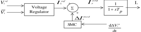
Equations (3.12) and (3.13) can be combined into a single complex equation as: converter and uses self commutating power semiconductor devices such as GTOs. The principle of working is similar to that of a synchronous condenser. The primary control in the STATCOM is reactive current control. The reactive current is controlled by firing angle control and it is a closed loop control as the reactive current is dependent on the system parameters, unlike in the case of SVC where the control is open loop because of the dependence of susceptance on firing angle alone. However, for stability studies involving low frequency oscillations, it is adequate to ignore the closed loop controller for the reactive current and assume that Ir

follows Irord with appropriate time delay (Figure 3.1).

STATCOM voltage regulator with supplementary modulation controller (SMC).The voltage regulator consists essentially of a PI-controller and the output of the controller Irref is modulated by the modulating signal

generated by the SMC Irord to enhance the damping of the

low frequency oscillations.It is to be noted that the work presented in this chapter does not consider the primary controller for STATCOM viz., the voltage regulator to regulate the bus voltage, as the emphasis is on the design and performance evaluation of the supplementary modulation controller for the STATCOM.

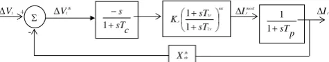
3.2.2 Control Structure

The general block diagram of the STATCOM supplementary modulation controller with phase compensating lead/lag network is show in Figure 3.2. In the figure, the feedback gain Xshth is the Thevenin reactance

of the STATCOM supplementary modulation controller which is tunable,

Vlis the magnitude of voltage at bus l where the controller

is connected,

Ir is the reactive current injected by the STATCOM into the

bus,

and Kr is the reactive current modulation controller gain.

mr denotes the number of stages of the compensating

© 2015, IRJET.NET- All Rights Reserved

Page 2266

compensation).The work presented in this chapter does not consider the phase compensating network.

The transfer function of STATCOM supplementary modulation controller with phase compensator is given by

th

Since the time delays associated delays associated with firing controls and natural response of the STATCOM can be represented by a single time constant the dynamics of the STATCOM is characterized by a first order plant supplementary modulation controller is given by

th

3.2.3 Tuning of STATCOM supplementary modulation controllers

The design parameters of the SMC for shunt and series FACTS controllers are the controller gain Kr and the

Thevenin reactance Xshth. The tuning of the SMC for

STATCOM can be viewed as getting the solution to a constrained optimization problem defined below:

j

n = total number of eigenvalues

σi = real part of the ith eigenvalue,

ωi= imaginary part of the ith eigenvalue,

Di = Damping ratio of the ith eigenvalue,

Wj = positive weight associated with the jth swing mode,

k = vector of control parameters, where each of the elements of the vector is greater than zero.

eigenvalues in the left half plane

The location of all the closed loop poles i.e., the eigenvalues of the system with SMC, on the boundary or within the sector shown in figure 3.3 will ensure that the constraints on damping ratio and the real part of the eigenvalues defined by equations (3.4) and (3.5) respectively are satisfied. The arbitrary choice of C1 and C2

may not result in a feasible solution. Hence the optimization problem. The problem formulation is based on sensitivity analysis of eigenvalues of the system. For a vector of small parameter increments Δk, the shift in the sth _{system mode can be written as}

s = gsRTΔk + j gsITΔk

(3.6)

where gsR and gsI are the gradients of the real and

imaginary parts of the eigenvalue s, given by

 

evaluated numerically by considering the (ij)th _{element of}

the matrix

of the vector k of control variables.

Based on the above equations, a linear programming problem is formulated at each step for tuning the supplementary modulation controller.

The LP problem is formulated as

© 2015, IRJET.NET- All Rights Reserved

Page 2267

(giRTΔk) M2i,

(3.10) Δkmax  Δk  Δkmin

(3.11) where





2 i i

ω

σ

ω

a







(3.12)





i i i

ω

σ

σ

ω

b







(3.13)

M1i = 1 – Di

(3.14)

M2i = -2 – σi

(3.15) and i = 1,2,….., n

(Note: Equations (3.9) and (3.10) are obtained by linearizing the equations (3.4) and (3.5) respectively.) The following algorithm is proposed for the design of FACTS supplementary modulation controllers:

1. Initial values of the design parameters ko are selected.

Initialize the counter p = 0, where p is the iteration number.

2. Eigenvalues of the system are computed. Select and track the mode of interest i.e., lightly damped swing mode whose damping is to be enhanced.

3. Since the constraints on damping ratios and real parts of all the eigenvalues cannot be achieved in one step of linear programming, initially set the minimum value of the damping ratio required to C1* _{= (Dmin +} _{1), and the}

maximum valued of the real part of the eigenvalues to C2*

= (σmax - 2), where

) ( _i i min min D D 

)

(

i

ma x

max

σ

σ



and 1 and 2 are greater than zero and small.

4. Compute ai and bi by applying equations (3.12) and

(3.13) respectively from the eigenvalues obtained in step 2. Also compute M1iand M2i from equations (3.14) and

(3.15).

5. The gradients are computed and sequential linear programming (SLP) problem is formulated.

6. If the LP is not feasible, set 1 = 1/2 and 2 = 2/2 and

check whether max [1, 2] <Tol (where the tolerance Tol

is a very small positive number). If the result is YES, set C1

= C1* _{and C2 = C2}* _{and stop. Otherwise go to step 3.}

7. If the LP is feasible, then update the parameters i.e., ko =

ko + Δk and the counter p = p + 1. Compute the

eigenvalues.

8. Check whether ΔDminC1 and (σmax) C2. If YES stop,

otherwise go to step 3. The above algorithm is explained in the flow chart shown in Figure 3.3.

The solution to the linear programming problem is obtained by making use of the Matlab optimization tool box [24] in the power system simulation program. It is to be noted that the number of iterations and hence the time taken to solve the SLP is mainly dependent on the initial values of the parameters and the lower and upper bounds on these parameters. If the increments Δk are too small, then the number of iterations will be large. But the large increments will diminish the accuracy of results. SMIB system data:

Eigen value analysis is crried out for the SMIB system without STATCOM and with the conventional STATCOM. Among the eigen values of the system without STATCOM a pair of eigen values lies on the right half of the complex plane, so the system is unstable, where all the eigen values of the system with STATCOM lie in the left half of the complex plane, which shows that the introduction of PSS stabilizes the system. By using the particle swarm optimization algorithm STATCOM parameters are tuned inorder to improve the eigen values obtained with STATCOM.

The bounds for the control parameters are shown in table 4.1 and Table 4.3 shows the STSTCOM Parameters obtained from the particle swarm optimization algorithm.

A STSTCOM has been used with speed as the input signal to damp this mode. The optimum value of the STATCOM gain is obtained by using particle swarm optimization algorithm. The optimum STSTCOM gain shown in Table 4.3 is chosen such that the real part of eigen value of the critical mode has maximum negative value, without destabilizing other mode. The value of washout time constant Tw is selected as 2.0 sec.

Table 4.4 shows the eigen values of the SMIB system with STSTCOM on the excitation system of the generator. The critical mode of interest is well damped with the real part of eigenvalue changing from 1.3831 to -4.1423, However there is a good improvement in the stability of the system with STATCOM-PSO compared to CSTATCOM.

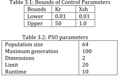
Table 3.1: Bounds of Control Parameters Bounds Kr Xsh

Lower 0.01 0.01 Upper 50 1.0

Table 3.2: PSO parameters Population size

Maximum generation Dimensions

Limit Runtime

© 2015, IRJET.NET- All Rights Reserved

Page 2268

Table 3.3: Optimal STATCOM Parameters Obtained From PSO

Kr Xsh

1.40000 0.140000

Table 3.4: Eigen values of the system with CSTATCOM and PSOSTATCOM

Eigen values of the system With

CSTATCOM

Eigen values of the system with PSOSTATCOM

-0.0010 +0.0015i

-0.000300116597859 +0.006341986115410i -0.0010

-0.0015i

-0.000300116597859 -0.006341986115410i -0.0000

+0.0007i

-0.000310630575709 +0.004358603483509i -0.0000

-0.0007i

-0.000310630575709 -0.004358603483509i -0.0003 -0.008089933105499

-0.0000 -0.002710052726282

V. RESULT AND DISCUSSION

A realistic power system is seldom at steady state, as it is continuously acted upon by disturbances which are stochastic in nature. The disturbance could be a large disturbance such as tripping of generator unit, sudden major load change and fault switching of transmission line etc. The system behavior following such a disturbance is critically dependent upon the magnitude, nature and the location of fault and to a certain extent on the system operating conditions. The stability analysis of the system under such conditions, normally termed as ‘transient-stability’ analysis is generally attempted using mathematical models involving a set of non-linear differential equations.

4.1Transient Stabilityanalysis

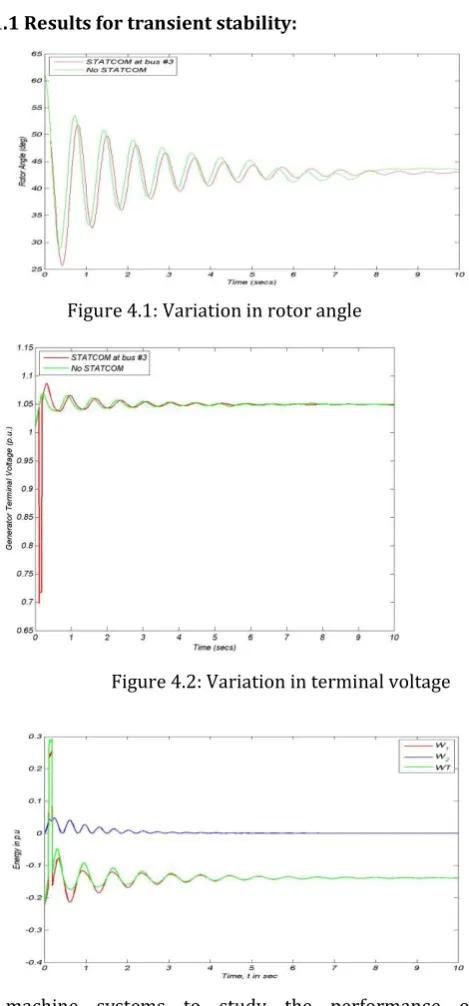
1.0 model is considered for the generators and the loads are treated as constant impedances. The system behavior is analyzed for three phase fault. The three phase fault is created on the critical bus 7 with a line outage. The fault is initiated at 0 sec and is cleared within 2.5 sec.

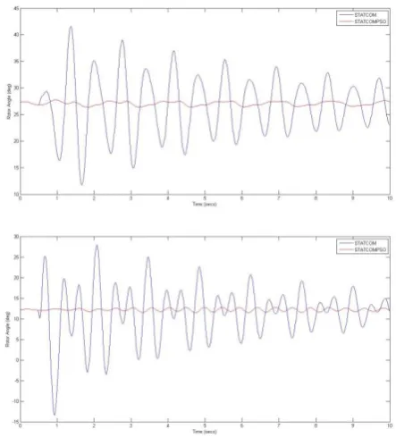
To improve the transient stability, simulation is performed with PSS and PSOPSS placed on generator as shown in Figures. The output of PSS can regulate the exciter voltage as a result of which the real power output of the machines and also the bus voltage variation at the critical buses have also reduced as shown in Figures. From the results it is clear that oscillations are damped and the system is stabilized at a faster rate compared to the conventional PSS.

4.1.1 Results for transient stability:

Figure 4.1: Variation in rotor angle

Figure 4.2: Variation in terminal voltage

3-machine systems to study the performance of STATCOM supplementary modulation controller with regard to the enhancement of damping of the low frequency swing mode. The generators are represented using detailed model 1.1 in all the systems. The results presented in this chapter concern the following objectives: i) Development of transient stability program using the STATCOM model described in the preceding sections in the presence of large and heavy disturbances.

ii) Direct evaluation of transient stability is conducted with STATCOM using the Ant Colony optimization method, which is incorporated in the transient stability program. Two types of fault studies are considered:

© 2015, IRJET.NET- All Rights Reserved

Page 2269

Both kinds of disturbances are cleared with line outage. Generalized MATLAB based programs have been developed using the models which have been described in the preceding sections. The programs have been implemented on Pentium(R) CPU system 3.40 GHz Table: 5.1 Values of STATCOM with PSO parameters

Kr Xsh

Val

ue 4.55090000 0000004

0.02960000 0000000

Table : 5.2 Eigen values of the multi machine system

Figure 5.1: optimum parameters of STATCOM using PSO

Figure 5.2: Eigen values of system at 3rd _generator

VI.CONCLUSION

This chapter has presented the Particle Swarm Optimization Algorithm for the design of power system stabilizers. The performance evaluation of the proposed stabilizer on a single machine system shows that increased robustness could be achieved by application of PSO to stabilizer design. The design procedure using PSO is also simple and can be used for particle implementation. The performance of the PSOSTATCOM is compared with CSTATCOM. PSOSTATCOM gives better performance compared to CSTATCOM.

References

Satheesh and T. Manigandan, ” Improving Power System Stability using PSO and NN with the aid of FACTS Controller” European Journal of Scientific Research ISSN 1450-216X Vol.71 NO.2 (2012), pp.255-164.

K. M. Passino, “Biomimicry of bacterial foraging for distributed optimization,” IEEE Control Systems Magazine, vol. 22, no. 3, pp. 52-67, 2002.

M. Faridi, H. Maeiiat, M. Karimi, P. Farhadi and H. Moslesh (2011) Power System Stability Enhancement

Using Static Synchronous Series Compensator (SSSC)‖ IEEE Transactions onPower System pp. 387- 391.

M. A. Abido, “Optimal power flow using particle swarm optimization” Proc. Int. J. Elect. Power Energy Syst., vol. 24, no. 7, pp. 563– 571, 2002.

Sidhartha Panda, and Narayana Prasad Padhy, “Comparison of particle swarm optimization and genetic algorithm for FACTS-based controller design” Applied Soft Computing, vol. 8, pp. 1418–1427, 2008.

Eigen values of the system

With Conventional STATCOM

Eigen values of the system STATCOM With PSO

-10.333417748538750 +14.260602992687263i

-0.000157221871016

+0.006441720975923i

-10.333417748538750-14.260602992687263i

-0.000157221871016

-0.006441720975923i -0.025357871733690

+6.776195009965491i

-0.003551129739837 +0.001681910974407i

-0.025357871733690-6.776195009965491i

© 2015, IRJET.NET- All Rights Reserved

Page 2270

Y. L. Tan and Y. Wang, “Design of series and shunt FACTS controller using adaptive nonlinear coordinated design techniques,” IEEE Transactions on Power Systems, vol. 12, no. 3, pp. 1374–1379, 1997.

Y. Wang, R. R. Mohler, R. Spee and W. Mittelstadt, “Variable-structure FACTS controllers for power system transient stability,” IEEE Transactions on Power Systems, vol. 7, no. 1, pp. 307–313, 1992.

Kumkratug, P., 2011b. Improving power system transient stability with static synchronous series compensator. Am. J. Applied Sci., 8: 77-81. DOI: 10.3844/ajassp.2011.77.81 K. M. Passino, “Biomimicry of bacterial foraging for distributed optimization,” IEEE Control Systems Magazine, vol. 22, no. 3, pp. 52-67, 2002.

P.Kundur, Power System Stability and Control, McGraw-Hill Press 1994.