Volume 2010, Article ID 345052,20pages doi:10.1155/2010/345052
Research Article
Collaborative Event-Driven Coverage and Rate Allocation for
Event Miss-Ratio Assurances in Wireless Sensor Networks
H. Ozgur Sanli and Hasan C¸am
Computer Science and Engineering Department, Arizona State University, Tempe, AZ 85287, USA
Correspondence should be addressed to Hasan C¸am,[email protected]
Received 2 November 2009; Accepted 30 March 2010
Academic Editor: Xinbing Wang
Copyright © 2010 H. Ozgur Sanli and H. C¸am. This is an open access article distributed under the Creative Commons Attribution License, which permits unrestricted use, distribution, and reproduction in any medium, provided the original work is properly cited.
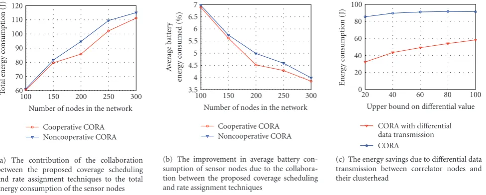
Wireless sensor networks are often required to provide event miss-ratio assurance for a given event type. To meet such assurances along with minimum energy consumption, this paper shows how a node’s activation and rate assignment is dependent on its distance to event sources, and proposes a practical coverage and rate allocation (CORA) protocol to exploit this dependency in realistic environments. Both uniform event distribution and nonuniform event distribution are considered and the notion of idealcorrelation distancearound a clusterhead is introduced for on-duty node selection. In correlation distance guided CORA, rate assignment assists coverage scheduling by determining which nodes should be activated for minimizing data redundancy in transmission. Coverage scheduling assists rate assignment by controlling the amount of overlap among sensing regions of neighboring nodes, thereby providing sufficient data correlation for rate assignment. Extensive simulation results show that CORA meets the required event miss-ratios in realistic environments. CORA’s joint coverage scheduling and rate allocation reduce the total energy expenditure by 85%, average battery energy consumption by 25%, and the overhead of source coding up to 90% as compared to existing rate allocation techniques.
1. Introduction
Wireless sensor networks usually consist of a large number of sensor nodes that collaboratively gather data from a target region of interest. A sensor network is expected to provide event miss-ratio guarantees, while minimizing the energy consumption of its sensor nodes. The miss-ratio for an event is equal to the fraction of those occurrences that are missed by wireless sensor nodes in a given time interval. While a sensor network can dynamically adapt its aggregate coverage in response to event misses, providing such assurances with minimum energy consumption is not easy due to the following problems. First, event occurrences may follow a nonuniform distribution. Consequently, two sensor nodes may detect a different number of events in a given interval even though their contribution to aggregate coverage of the network is the same. Second, minimizing the number of active nodes by reducing the overlapping areas among sensing regions of neighboring nodes often sacrifices their correlation. However, sensor data correlation can be exploited by distributed source coding for reducing
the energy spent for data transmission which is a major com-ponent in overall system energy consumption [1,2]. Inspired by these problems, this paper is the first of its kind to exploit the relationship between coverage scheduling (i.e., deciding which sensing unit(s) of each node should be activated) and source coding rate allocation (i.e., determining the number of bits that a sensor node should transmit for its sensor reading), and to show how they should cooperate. The main contributions of this research include the following.
(1) We demonstrate the existence of an idealcorrelator radiuswithin cluster of sensor nodes around which on-duty node selection will minimize the amount of data sensed and transmitted under both uniform and nonuniform event distributions.
event miss-ratio assurances even when nodes have no location information and there’s noise in sensing ranges of nodes.
(3) This paper develops a novel technique calleddiff er-ential data transmissionto remove those data redun-dancies which cannot be eliminated via distributed source coding. Nonredundant data gathered by dis-tributed source coding are compared with known reference data and then only its difference from the reference data are transmitted to the clusterhead.
We noticed that certain cluster members are critical for meeting the required event miss-ratios energy efficiently due to their following two features. First, by taking advantage of their location in cluster topology, they can apply distributed source coding for other cluster members and significantly reduce data redundancy. Second, due to their proximity to the hotspots (i.e., regions with high event occurrence prob-abilities), they can detect majority of the event occurrences which are condensed around hotspots. Therefore, in CORA, rate allocation requests coverage scheduling to activate such critical cluster members within the ideal proximity of the clusterhead which we refer as correlator radius. Similarly, coverage scheduling helps rate allocation assign various rates to sensor nodes by determining which neighboring sensor nodes of a given sensor node should be put in sleep mode.
CORA’s rate allocation first identifies the uniform/ nonuniform distribution of event occurrences using a continuously updated histogram. Under nonuniform event distribution, those hotspot locations where the event occur-rence probability is very high are determined. For both uniform and nonuniform event distributions, we then demonstrate the existence of an ideal radius around the clusterhead where the source coding gain is maximized. At the distance of ideal radius from clusterhead, our rate allocation algorithm forms groups of active nodes. Each group has a so-calledcorrelator nodethat gathers data from its group members and transmits the aggregated data to its clusterhead. To further improve data reduction, we propose a new differential data transmission technique for correlator nodes. To the best of our knowledge, there is no previously known technique that assigns rates in accordance with the occurrence of the observed phenomena.
CORA’s coverage scheduling is unique of its kind in guaranteeing the miss-ratio required for each event without any need for location information of nodes. While activating less number of nodes than existing coverage scheduling algorithms to provide such assurances, coverage scheduling also relieves sensor nodes computation and storage overhead. To be of practical value, the coverage scheduling algorithm takes into account the effects of realistic environments on coverage such as the changes in sensing ability of nodes and the noise in distance measurements between node pairs.
The preliminary results of this research have appeared in [3,4]. The rest of the paper is organized as follows. The related work is presented inSection 2. InSection 3, system model and assumptions are given. The problem we tackle is formally described inSection 4.Section 5presents the CORA
protocol. The performance evaluation of CORA is discussed inSection 6. The concluding remarks are made inSection 7.
2. Related Work
Coverage scheduling algorithms and distributed source coding techniques are usually addressed as two separate research fronts in the literature. CORA distinguishes itself from the existing solutions in closing the loop between these two research fronts.
Coverage Scheduling. Coverage scheduling in wireless sensor networks has received increasing attention in the recent years [5–15]. Some research efforts have considered coverage scheduling in conjunction with connectivity requirements [16,17], bandwidth constraints [18], and target localization [19]. But, in none of the previously known coverage scheduling techniques, the impact of coverage scheduling on distributed source coding is addressed, even though distributed source coding efficiency depends on which set of sensor nodes gather data for an event. In comparison, CORA identifies the nodes that are critical for distributed source coding by keeping track of the event distribution. Then, only such critical nodes are put on duty to provide the variable coverage needed over the monitored area for minimizing event misses. CORA also uses less number of active nodes to meet the coverage needed than existing coverage scheduling techniques [5].
Rate Allocation. Distributed source coding [20, 21] and explicit communication [22] reduce the amount of data transmitted by taking advantage of the correlation structure between the sensor measurements. Let X and Y be the data sources at two neighboring sensor nodes that have overlapping sensing areas and belong to the same cluster. In case of distributed source coding, the data ofXare sent as
H(X) to the clusterhead which then informs Y about the correlation structure between the data ofX andY. Finally, the data ofYare encoded asH(Y|X) with side information
Xin accordance with the Slepian-Wolf theorem [20]. In case of explicit communication, the node with sourceY receives explicit side information H(X) from the node with source
X and decodes H(X). Then, the data of Y is encoded as
H(Y|X) and sent to their clusterhead in addition toH(X). Recently, rate assignment algorithms are developed to determine the coding rates to be used by each sensor node [22–24]. These rate assignment algorithms usually focus on minimizing energy consumption and do not consider the overhead of distributed source coding. In CORA however, cooperative coverage scheduling and rate assignment acti-vates and maintains correlation information only for those critical nodes that would maximize the energy saving of distributed source coding.
correlator radius, our rate allocation algorithm partitions on duty nodes into groups, each with a designated correlator node, and assigns rates within each group in response to the uniform/nonuniform distribution of event occurrences.
Rate allocation and network lifetime are very related to each other. For instance, in [25], rate allocation in wireless sensor networks is addressed under a given network lifetime requirement. This research work advocates the use of lexicographical max-min rate allocation for all sensor nodes in order to avoid a severe bias in rate allocation when the objective is to maximize the sum of rates of all nodes.
Event Miss-Ratio Assurances. The problem of event-misses have been addressed by several node level scheduling algo-rithms [26–29]. The objective of such research efforts is to keep a node in low power modes as much as possible while processing event occurrences within their deadlines. However, these existing techniques do not provide any event miss-ratio assurances and schedule events at a sensor node separately from its neighboring nodes. Such algorithms can not relieve a sensor node from processing those events that are also detected by its neighboring nodes. In comparison, CORA assigns each event only to some sensor nodes within a group of cluster members. Therefore, CORA significantly reduces the event processing load at each node.
3. System Model and Terminology
Network and Node Model. This paper focuses on dense wireless sensor networks which consists of multiple clusters that are formed based on node residual energy levels. We consider single hop clusters where each cluster member is within the direct transmission range of the clusterhead. The sensor nodes are static and have the same hardware capabilities. The distance between any two sensor nodes within a cluster is assumed to be known based on standard methods such as Received-Signal-Strength-Indicator (RSSI) and Time of Arrival (ToA).
We consider the recent commercial off-the-shelf sensor nodes that have multiple sensing units [30]. The sensor nodes do not have an attached GPS device but their positions within a cluster are estimated based on internode distances. The power control circuit of each sensing unit enables putting it in sleep or active mode [31]. The sensing unit consumes constant power level in active mode. The radio unit has dynamic transmission power control capability which enables sensor nodes to control their transmission range under the effect of environmental factors and multi-path propagation. In order to transmit nbits between two sensor nodes separated by a distance, the required power is modeled asn(a2+b) for transmission andnbfor reception whereaandbare constants [32].
Coverage and Event Model. In sensor networks, different types of coverage models exist, (i) the monitored area consists of a discrete set of points and each point should be within the sensing region of at least one active node [12], (ii) the monitored area is a predefined contiguous region and
the active sensor nodes should be covering each point within this region [10], and (iii) the monitored area is a contiguous region defined by the union of all individual nodes’ sensing regions, and a subset of active nodes should cover the sensing regions of others [11]. In this paper, we focus on the third coverage model. We consider both uniform and nonuniform event distribution models. In uniform case, each node has the same event occurrence probability. To model nonuniform event distribution, however, random hotspot locations are created within the monitored area, and event occurrences follow the Gaussian distribution around these hotspot locations.
Data Correlation Model. For n active sensor nodes that participate in source coding within the same group, a vector
μofnentries keeps the mean values of their sensor readings and an (n×n) matrixΓmaintains their correlation.μ(−→X)= (μ(X1),μ(X2),. . .,μ(Xn))T, where the random variable Xi
corresponds to the source sensor readings atith active cluster member for 1≤i≤n.Γ(i,j) denotes the correlation degree betweenith andjth active cluster member for 1≤i,j≤n.
The existing research efforts consider only internode distances while modeling sensor data correlation [33]. Given a set of nodes {X1,. . .,X(i−1)}, their model calculate the nonredundant data produced by node Xi based on the
minimum Euclidean distance between nodeXiand any node
Xjfor 1≤j≤(i−1). However, this distance-based approach
faces problems when nodeXiis very close to more than one
member of the node set {X1,. . .,X(i−1)}. In this case, the amount of nonredundant data generated by Xi is actually
much less than the amount that is approximated by their model. To address such cases and represent correlation more accurately, this paper models the data correlation among sensor nodes based on the overlapping area of their sensing regions. Specifically, the data correlation of active cluster membersiandjis expressed asΓ(i,j)=Area(Si∩Sj)/πrs2,
where Si andSj denote the sensing regions ofith and jth
active cluster members, respectively, for 1≤i,j≤nandrsis
the sensing range.
The total number of bits in the sensed data of a group ofn
sensor nodes is expressed based on their aggregate coverage. Specifically, if the entropy [34] of the source at a single cluster member is nB bits then the sensor nodes produce (nB ×
(Area(∪n
i=1Si)/πrs2)) bits of nonredundant data where Si is
the sensing region of nodeith sensor node for 1≤i≤n. The number of entries inμandΓindicate thestorage overheadof source coding which is equal to (n×1) + (n×n). Theupdate overheadof source coding is determined by the modifications made onμandΓfor each new event occurrence.Table 1lists most of the notation used in the rest of the paper.
4. Problem Statement
Let us consider an event typeMto be sensed by a wireless sensor network. Let us assume that a discrete set ofnsensor nodes’ sensing areas define the monitored area. Also let
xi denote the point where ith sensor node is located for
Table1: Notation.
rt The transmission range of any given node.
rs The sensing range of any given node.
S The sensing region of any given node.
M An event to be sensed by the wireless sensor network. K The set of sensor nodes in any given cluster.
nK The number of sensor nodes in any given cluster.
Ki ith sensor node in any given cluster where 1≤i≤nK.
Area
(X) Area of any given regionX.
H(Y) The entropy of any given random variableY[34].
nB The number of bits needed to represent a sensor reading. If the sensor source at any given node is denoted byXis thennB=H(X).
one event can occur at location xi. We define two random
variablesY andDthat correspond to the total number of eventoccurrencesand the total number of eventdetections, respectively, within the monitored area. When the monitored area has total k event occurrences,Y assumes the value k
for 0 ≤ k ≤ n. Similarly,Dtakes the value when total
event occurrences are detected amongknumber of event occurrences for 0≤≤k≤n. Also let us define the inputs and outputs of the problem as follows.
(i) Inputs:
(a)γreq: the required event miss-ratio threshold for eventM,
(b)ai: the sensing area of sensor node at locationxi
for 1≤i≤n,
(c) Prob(oi): probability of event occurrence atai
for 1≤i≤n,
(d) Prob(Y = k): probability that Y takes valuek
for 0≤k≤n.
(ii) Outputs:
(a)γobs: the observed (actual) event miss-ratio for eventM,
(b) Prob(di): probability of event detection ataifor
1≤i≤n,
(c)ei: the energy consumption of active sensor
nodes for data transmission with their assigned rates at locationxifor 1≤i≤n,
(d) Prob(D = ): probability thatDtakes value
for 0≤≤k≤n.
The problem of this paper is to show that the proposed protocol CORA guarantees that the observed event miss-ratioγobsis less than or equal to the required event miss-ratio
γreq
Observed event miss-ratioγobs
=
1−E(D)
E(Y)
≤
Required event miss-ratioγreq
,
(1)
and minimize the total energy consumption of all active sensor nodes
Minimize
n
i=1
ei, (2)
whereE(D) andE(Y) (i.e., the expected values ofDandY, resp.) are written as
E(D)=
n
=0
[×Prob(D=)],
E(Y)=
n
k=0
[k×Prob(Y=k)].
(3)
There are two extreme cases for γobs. At one extreme, the observed event miss-ratio is becoming equal to one when all event occurrences are missed. The other extreme occurs when all event occurrences are detected, thereby making the observed event miss-ratio equal to zero.
Among the aforementioned probability values,
textProb(oi) depends on the distribution of event
occurrences. Prob(di) is controlled by the aggregate
coverage of active sensor nodes. Prob(Y=k) is computed by considering all possible combinations of thenlocations for having totalkevents in the monitored area for 0≤k≤n. As an example, let us derive a close expression for Prob(Y =1) where there exists a single event in the entire monitored area. The probability, saypi, that a single event occurs at location
iis equal to the probability of event occurrence at location
itimes the product of all those probabilities of not having event occurrences at the remaining (n−1) grid locations for 1≤i≤n. Prob(Y =1) is equal to the sum of allpis overn
locations. Thus,
Prob(Y =1)=
n
i=1 ⎡
⎣Prob(oi)× n
h=1,h /=i
(1−Prob(oh))
⎤ ⎦. (4)
Since there is no close formula for Prob(Y =k) for 2≤k≤
Require:Y=k: The case of having totalkevent occurrences in the monitored area where 0≤k≤nandnis the number of sensor locations.
Ensure:Prob(Y=k) is computed. 1: Initialize Prob(Y=k)=0.
2: Determine the setAof all possible combinations ofkevents that occur in anykout ofnnetwork locations. 3:whilethe setAis not emptydo
4: Remove a combination fromAand denote it byC.
5: Find out the product of the event occurrence probabilities at the locations selected by combinationCand probabilities of not having any event occurrences at the remaining locations of the network.
6: Multiply the product from the previous step with the probability of having combinationCand add the result of multiplication to Prob(Y=k).
7:end while
Algorithm1: Probability computation forY.
Monitored area
0 20
40 60 80
X(m)
20 40 60 80
Y(m)
0 0.2 0.4 0.6 0.8 1
P
robabilit
y
o
f
ev
ent
oc
cur
re
n
ce
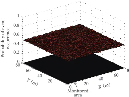
Figure 1: A uniform event distribution is shown for the black colored monitored area. A nonzero event occurrence probability at any point is indicated in red color.
the probability of event occurrences but also their probability of detection. For example, Prob(D=1) is expressed as
Prob(D=1)=
n
i=1
(Prob(oi)×Prob(di))×Wi
, (5)
where
Wi= n
h=1,h /=i
(1−Prob(oh)Prob(dh)). (6)
5. CORA Protocol for Event
Miss-Ratio Assurances
We first give in this section an overview of how CORA provides event miss-ratio assurances with minimum energy consumption. The network lifetime is divided into consec-utive roundsand CORA performs coverage scheduling and rate assignment at the beginning of each round. The round-based operation enables CORA to take the recent node residual energy information into account. At each location
xi, coverage scheduling and rate assignment control Prob(di)
andei,respectively, for 1≤i≤n. Meanwhile, CORA enables
event-driven cooperation of coverage scheduling and rate assignment in two phases.
In Phase I, event distribution is identified using a continuously updated histogram. Depending on whether the event distribution is uniform or nonuniform, the ideal correlator radius is found for each cluster. As we will show, there exists a single correlator radius within the cluster for uniform event distribution such as the one depicted in Figure 1. For nonuniform event distributions as illustrated inFigure 2, a local correlator radius exists for each hotspot. The local correlator radii of all hotspots are combined to find the cluster level global correlator radius. Under the guidance of the correlator radius, correlator nodes are selected and cluster members form groups around correlator nodes for rate assignment.
In Phase II, those critical nodes which significantly improve the energy consumption of the cluster are identified from their assigned rates. Coverage scheduling then activates only those critical nodes for improving energy consumption and meeting the required event miss-ratios. Since Phase I differs for uniform and nonuniform event distributions, the steps ofPhase Iare described next separately for uniform and nonuniform event distributions.
5.1. Phase I for Uniform Event Distribution. The expected amount of data generated by each node is the same under uniform event distribution. Therefore, the locations of sensor nodes within the cluster topology plays the key role for overall energy consumption. In this section, we study how distance of correlator nodes to the clusterhead affects the energy expenditure. Let us refer to this distance asrcwhere
the subscript denotes thecorrelator radiusand 0 ≤rc ≤rt.
Letrc∗be theidealrcvalue which maximizes the energy gain
of distributed source coding by correlator nodes relative to the case when cluster members transmit data directly to the clusterhead. In what follows, we will explain howrc∗is found
in Step I of Protocol CORA by formulating this energy gain as a function of rc. We will then describe the allocation of
Require:M: An event to be sensed by sensor nodes in a cluster-based wireless sensor network. γreq: The required event miss-ratio threshold.
Ensure:i) The event miss-ratio assuranceγobs≤γreqis met.
ii)ni=1eiis minimized.
{PHASE I}
Step I: Each clusterhead finds its correlator radius.
Step II: Those cluster members that are located around the correlator radius form rate assignment groups, each consisting of a correlator node and a number of sensor nodes.
Step III: Each correlator node assigns the source coding rates to its group members in order to minimizeni=1ei.
{PHASE II}
Step IV: Each clusterhead identifies the critical nodes of rate assignment groups, based on their assigned rates.
Step V: The members of each cluster perform coverage scheduling by activating critical nodes, in order to meet the required event miss-ratio thresholdγobs≤γreq.
Algorithm2: Protocol CORA.
Monitored area
0 20
40 60 80
X(m) 20
40 60 80
Y(m)
0 0.2 0.4 0.6 0.8 1
P
robabilit
y
o
f
ev
ent
oc
cur
re
n
ce
Figure 2: A nonuniform event distribution is shown for the
monitored area illustrated in black color. A nonzero probability of event occurrence at any point is depicted in blue color.
We now analyze the energy consumption for a cluster of wireless sensor nodes when distributed source coding is applied at a given distancercfrom the clusterhead (i.e., when
correlator nodes have distance rc to the clusterhead). The
first question we answer in this analysis is the following: For which cluster members would correlator nodes yield any improvement in energy consumption? Especially within the close proximity of the clusterhead, transmitting data directly to the clusterhead (i.e., bypassing the correlators) should be preferable over sending data through the correlator nodes.
Let us call the union of those locations from where the sensed data should be sent directly to the clusterhead as Direct Transmission Region (DTR). Letrddenote the radius of
DTRwhere the subscriptdrefers to direct data transmission. The donut shaped region obtained by excluding the DTR
from the clusterhead transmission region is referred to as Distributed Source Coding Region (DSCR).Figure 3illustrates
DTRandDSCRin blue and red colors, respectively. To identify DTR, we find the relationship between rd
and rc. Specifically, we consider the energy consumed for
gathering data from any cluster member Ki with distance
rd to the clusterhead where 1 ≤ i ≤ nK. Note that the
energy consumption of nodeKishould be the same in direct
data transmission and distributed source coding cases since node Ki is located on the boundary of DTR. Let us refer
to the energy consumption of nodeKi when it uses direct
transmission to the clusterhead asedirect. Leteindirectbe the energy consumption ofKiwhen its data reach the clusterhead
indirectly through correlator nodes.
When node Ki bypasses the correlators, the entropy
of the source at node Ki is transmitted over distance rd
to the clusterhead. Based on the energy model given in Section 3,edirectwould be
edirect=nB
ar2d+ 2b
. (7)
When correlator nodes apply distributed source coding at distancerc from the clusterhead,Ki sends only
nonredun-dant data to the correlator node which are then forwarded to the clusterhead. Thus, we next consider the expected amount of data transmitted by node Ki when data redundancy is
eliminated by distributed source coding.
The redundancy in node Ki’s data is attributed to the
overlap of nodeKi’s sensing region with the sensing regions
of its neighboring nodes. Consequently, we need to find how much of the area within the sensing range of a node is covered only by the node itself. When there is coverage redundancy within the cluster, the expected size of the common area covered by nodeKiwith its neighboring nodes
is
nKπrs2−π(rt+rs)2
nK
, (8)
where π(rt+rs)2 refers to the coverage area of the cluster
and the term nKπrs2 denotes the maximum area that can
Cluster
Figure3: A correlator nodeYis illustrated with its membersX1,X2,
and X3. The ideal correlator radius rc∗ guides the formation of
such rate assignment groups in Distributed Source Coding Region (DSCR) shaded in red color. The cluster members such as node X4 in blue colored Direct Transmission Region (DTR) send data
directly to the clusterhead.
coverage redundancy is uniformly distributed among cluster members,ωis expressed as
ω=
Let us also assume that the task of covering the common areas (i.e., the regions that are covered by at least two cluster members) is evenly distributed among all cluster members. We introduce the variable β as the expected ratio of the common areas covered by a sensor node to its overall sensing region where 0 ≤ β ≤ 1. Since any area within the cluster that is not covered only by a single sensor node belongs to the common area,βis expressed as
β=
From the exclusive and common areas covered by nodeKi,
we can now determine the amount of nonredundant data transmitted by nodeKiand expresseindirect. Specifically,
eindirect=
whereεrepresents the ratio of the rate control message size to the data message size. First, rate information is transmitted from the correlator to node Ki over distance (rc −rd).
Then, nodeKicodes sensor data with the assigned rate. The
data received by the correlator node are transmitted to the clusterhead over distancerc.
Let rd(rc) refer to the rd value substitution of which to (7) and (11) yields the same energy consumption foredirect and eindirect, respectively. The term rc is included in rd(rc) subscript to indicate that rd is dependent on therc value.
Sincerd(rc)refers to the radius ofDTR, a cluster member uses direct data transmission to the clusterhead if its distance to the clusterhead is less thanrd(rc). Otherwise, the data of the cluster member are sent to its designated correlator node. In light of this selection criteria for data transmission, we next define the energy gain function of correlator nodes for any givenrcvalue.
Let ensc denote the energy consumption for gathering data from the cluster members when they bypass the correlator nodes and transmit their data directly to the clusterhead with the subscript referring to no source coding. Letedscbe the energy expenditure for the case where cluster members use correlator nodes with the subscript denoting distributed source coding. edsc is a function of rc and is
defined within the interval [0−rt] whileenscis independent fromrc. Then, theenergy gaindue to the correlator nodes is
defined asegainwhere
egain=ensc−edsc. (12)
By incorporating each possible location of a cluster member within the cluster,edscis expressed as
edsc=(A+B), (13)
whereAandBrefer to the expected energy consumption of cluster members inDTRandDSCR, respectively. Specifically,
A=
a sensor node with distancer to the clusterhead. The first and second terms of (14) represent the energy consumption of cluster members inDSCRthat are closer to and farther from the clusterhead than correlator nodes, respectively. On the other hand,ensc is defined by considering the direct transmission from each cluster member as
ensc=
By subtractingedscfromensc,egainis determined and the ideal correlator radius is found as the rc value which yields the
maximumegain. Specifically,egainis a dome-shaped function ofrcwith its derivative having value zero at pointrc∗.Figure 4
Require:A cluster of sensor nodes that produce correlated data for a given eventM.
Ensure:The coding rates are allocated for eventMto minimize the energy consumption. 1: The ideal correlator radiusr∗
c is determined by the clusterhead for uniform event distribution.
2:for allActive nodeKi, 1≤i≤nK do
3: if Kiis located withinDTRthen
4: Use coding rateRKi=H(Ki) and transmit data directly to the clusterhead. 5: else
6: Check whether nodeKishould become a correlator node by verifying the residual energy requirement and comparing its
distance to the clusterhead withr∗
c.
7: if Kiis selected as correlatorthen
8: Code data at rateRKi=H(Ki) and apply differential data transmission for group members.
9: else
10: Use coding rateRKi=H(Ki|Ψ) and send data to the correlator node where the setΨcontains the group members with higher residual energy.
11: end if
12: end if
13:end for
Algorithm3: Coding rate assignment.
30 25 rc∗
15 10 5
0
rc(m) 2.8
3 3.2 3.4 3.6 3.8
×104
egain
(J
)
Figure 4:egain is shown for a cluster of 500 sensor nodes with
settingsrs=10 m.,rt=30 m. (i.e., cluster range),nB=16 bits and
ε=0.2. The ideal correlator radiusrc∗within the interval [0−rt] is
indicated with the dashed blue line.
Algorithm Coding Rate Assignment describes how rate allocation groups are formed under guidance of rc∗ and
rates are assigned to group members at Step II and Step III of Protocol CORA, respectively. To select the correlator nodes, the average residual energy of cluster members is calculated first. A cluster member within DSCR becomes a correlator node if (i) it has higher residual energy than the average residual energy, and (ii) its distance to the clusterhead is closer tor∗c than any one of its neighboring
nodes. The remaining active nodes join the group of the closest correlator node.
Within each group, the data transmissions from group members to the correlator node are ordered in descending order of node residual energy levels. Thus, a sensor node uses the data of other group members that have higher
residual energy as side information. Note that, having a high residual energy node transmit data earlier than others does not guarantee that it will use the highest coding rate. This is especially true when such a node has highly overlapping sensing region with other high energy nodes that have already transmitted data. However, when a high energy node uses low coding rate, its residual energy would not change significantly while other nodes would be spending more energy. Consequently, CORA would schedule such group members to transmit data earlier than others in the following rounds.
The correlator node applies the proposed differential data transmission technique to further reduce the size of the data before sending it to the clusterhead. The basic motivation behind differential data transmission is that the data gathered from group members exhibit not only spatial correlation but also temporal correlation. To exploit the correlation in temporal domain, both clusterhead and correlator node maintain a common reference data which captures the characteristic values of last ndata values transmitted from the correlator node to the clusterhead.
LetRbe the reference data andW be the raw nonredun-dant data gathered at the correlator node. Letdenote the difference operator and⊕refer to its inverse. As an example, if the sensor readings are mapped to numbers thanand⊕ may correspond to the subtraction and addition, respectively. Then, the correlator node transmits the differential data
D with the value D = (W R). After receiving D, the clusterhead recovers the original raw dataW=(D⊕R).
Cluster-head for the sensor node
Figure5: The analysis of energy consumption for a hotspot that is located at the origin. The hotspot has distancedto the clusterhead and correlator radiusrcis used within the cluster.
computation of the ideal correlator radiusrc∗ for a hotspot
with distancedto the clusterhead as shown inFigure 5. In the analysis, we do not follow a particular event distribution but assume that event occurrence probabilities are nonzero within the local proximity of hotspots only. In particular, let Prob(er) be the event occurrence
prob-ability at a point with distance r to the hotspot center. Prob(er) can be calculated either by using exponential and
Pareto distributions depending on the nature of the event occurrences. In exponential distribution, the probability density function is Prob(er) = (ae−ar) where the event
occurrence probability decreases rapidly as the distance to the hotspot center increases. For those hotspots with a slowly decreasing effect, Pareto distribution is more suitable due to its density function Prob(er) = (aka/ra+1) where a is the
shape parameter andkis the initial value.
As in uniform event distribution analysis, we will express the energy gain functionegainin terms ofrcwhere 0 ≤rc ≤
d. However, unlike the uniform event distribution case, the analysis is shaped by those locations near hotspots that have nonzero event occurrence probabilities rather than all cluster locations. Let us refer to the maximum distance between the center of the hotspot and any node within the hotspot as the hotspot rangeand denote it bydHS.
In computation of bothedsc andensc, we will consider each possible distancer that a sensor node can have to the hotspot center where 0 ≤ r ≤ dHS. In Figure 5, a red circle labeledCrillustrates the possible node locations with
distance r to the hotspot center. For the upper semicircle of Cr as an example, such locations are defined by the
coordinates (x,y) where −r ≤ x ≤ r and y = √r2−x2. Let edsc(r) denote the expected energy consumption of the nodes located on Cr when they use correlator nodes. Let
ensc(r) refer to the expected energy expenditure of the same nodes onCrwhen they apply direct data transmission to the
clusterhead. We will integrate edsc(r) and ensc(r) over all Cr
within the hotspot to findedscandensc, respectively.
To computeedsc(r), we break upCr into small segments
dswith each segment representing a possible location of a sensor node onCr. For each one of these segments, the event
occurrence probability is the same and is equal to Prob(er).
FromFigure 5, it can be observed that
ds= dx2+d y2=
sensor node onCr, the probability of event data transmission
fromdsis equal to the probability that the node is placed atds(i.e.,ds/2πr)andthe probability that an event occurs (i.e., Prob(er)). The energy consumption for sending data
fromdsto the clusterhead consists of two components. First, the data are transmitted from ds to the correlator node over distance dc, and then sent by correlator node to the
clusterhead over distancerc.
To determineensc(r), we follow the same segment-based division of Cr but assume that any sensor node on Cr
bypasses the correlator nodes. Thus,
ensc(r)=2
To express edsc andensc, we integrate over each r and incorporate the expected number of nodes to be located on
Crfor 0≤r ≤dHS. Specifically,
Finally, we take the derivative of the energy gain functionegain whereegain=ensc−edsc. The ideal correlator radiusrc∗makes
the derivative functionegainequal to zero at pointrc∗.
Given a set ofkhotspots with the local ideal correlator radius for the jth hotspot referred to as rc∗(j), the global
ideal correlator radius is set as rc∗ =
k
j=1rc∗(j)/k where
1 ≤ j ≤ k. Once the value ofrc∗ is obtained, the selection
Require:A cluster of wireless sensor nodes to be scheduled for sensing eventM. γreq: The required event miss-ratio threshold for eventM.
χ: The scores assigned to cluster members based on coding rate estimates.
Ensure:Each cluster member is selected either as an active node or a sleeping node for eventM. 1: The setKof cluster members are sorted in ascending order of their scores inχ.
2:for allNodeKi, 1≤i≤nK do
3: Prob(di) is identified fromγreqand event distribution forM.
4: ifProb(di) is met by neighboring nodes of nodeKi then
5: NodeKigoes to sleep mode.
6: else
7: NodeKiis activated forM.
8: end if
9:end for
Algorithm4: Coverage scheduling.
those group members that are near the hotspots consume more energy due to their high event detection activity. Thus, CORA alleviates the burden on such nodes by increasing their side information in distributed source coding.
5.3. Phase II for Both Uniform and Nonuniform Event Distributions. This section presents the steps of Phase II that are implemented in the same way for both uniform and nonuniform event distributions. CORA employs a priority-based coverage scheduling technique to select the active sensor nodes for each event M. In coverage scheduling, a node that is considered earlier for activation has better chance of going to sleep mode since those nodes that are waiting to be activated can still meet the required event miss-ratio. Based on this observation, CORA implements node priorities to have critical nodes considered later in coverage scheduling, thereby forcing them to remain active. In Step IV, each cluster memberKiis associated with a scoreχithat
reveals how much it improves the energy expenditure of the cluster for 1≤i≤nK.χiis computed by estimating the rates
within the neighborhood of nodeKi for the following two
cases:
Case I. NodeKiparticipates in distributed source coding.
Case II. NodeKiis excluded from distributed source coding.
The rate predictions are made according to the proposed rate assignment algorithms. Then,χiis set as the ratio of the
expected average residual energy of the neighboring nodes for Case I to the one for Case II. Consequently, the critical nodes get assigned the highest scores.
Algorithm Coverage Scheduling implements Step V of Protocol CORA for the assignment of events to cluster members. The clusterhead first sorts the nodes in ascending order of their scores such that low score nodes are considered first. Then, each nodeKiis evaluated for coverage scheduling
in the order of its score where 1≤i≤nK. The status of node
Kifor eventMis determined according to its sensing region’s
overlap with the sensing regions of its neighboring nodes. To control event misses, either (i) nodeKi remains active and
covers the physical area within its sensing region on its own,
or (ii) nodeKi goes to sleep mode and lets its neighboring
nodes provide coverage over its sensing region.
LetUdenote the set of neighboring nodes forKithat can
contribute to the coverage ofKi’s sensing region where 1 ≤
i ≤ nK. Based on the evaluation of scores, the clusterhead
creates aneligible set of neighboring nodesUe for coverage
of nodeKi’s sensing region whereUe⊆U. Each neighboring
nodeK∈Uesatisfies either one of the following conditions
where 1≤≤nKandi /=.
(i)χ > χi.
(ii)χ =χiand nodeKhas already been scheduled as an
active node or has not announced its status yet forM. (iii)χ < χiand nodeKhas already been scheduled as an
active node forM.
Once its eligible set of neighboring nodes are identified, node
Ki computes the uncovered part of its sensing region for
eventMdenoted byαwhere 0≤α≤1. Ifα≤(1−Prob(di)),
then node Ki goes to sleep mode for event M since its
sensing region is covered sufficiently by neighboring nodes that would remain active. Otherwise, nodeKi is scheduled
active to preserve Prob(di) for eventM.
To ensure that γobs ≤ γreq, each cluster member Ki
identifies its Prob(di) fromγreq and event distribution such that 0≤(1−Prob(di))≤γreq. Let us define Prob(omax) and Prob(omin) as the maximum and minimum probability of an event occurrence, respectively, forMat any point within the monitored region. Specifically, Prob(omax)=max(Prob(oi))
and Prob(omin)=min(Prob(oi)) for 1≤i≤nwherenis the
sensor locations in the monitored region. For nodeKilocated
atxi, Prob(di) is set as
Prob(di)=1−γreq $
1− (Prob(oi)−Prob(omin)) (Prob(omax)−Prob(omin))
% , (21)
where 1 ≤ i ≤ n. Consequently, CORA provides variable coverage over the monitored area with the worst and best coverage defined by the following two cases. When Prob(oi)
is equal to Prob(omin), node Ki meets the required event
miss-ratio threshold by setting Prob(di)=(1−γreq). On the other hand, if Prob(oi) is equal to Prob(omax), then nodeKi
Node 1
rg
ρ
Lowest id segment Node 2
rs
Figure6: An example where the sensing region of nodes are divided intonG = 6 segments. The covered portion of each segment by
neighboring nodes is represented with an angle. In the figure,ρ corresponds to the covered portion of the lowest id segment,Sl5,
of node 1’s sensing region by its neighboring node 2.
Lemma 1. The variable coverage provided by CORA
guaran-tees thatγobs< γreq for any given eventM.
Proof ofLemma 1.The proof is given in the Appendix.
We next present an efficient algorithm to compute the area covered within a node’s sensing region by its neigh-boring nodes. The coverage computation is used to verify that a node’s sensing region has sufficient overlap with its neighboring nodes before the node goes to sleep mode. While computing coverage, a sensor node considers its neighboring nodes in ascending order of their identifiers. For each neighboring node, the area of intersection that’s not covered by lower id nodes is determined. This helps the overlapping areas between the sensing regions of neighboring nodes to be considered only once.
Algorithm Coverage Computation describes the steps taken for finding the area of overlap a node has with its neighboring nodes. The sensing region of each node is represented as a set of nG segments {Sl1,Sl2,. . .,SlnG} as shown inFigure 6wherenG≥1. Each segment has the same
thickness rg and the union of all segments is equal to the
node’s sensing region wherers=nG∗rg. The segments are
numbered in increasing order from the center of the sensing region towards its boundary.
For a given neighboring node, the segment with the lowest id that intersects with the sensing region of the neighboring node is determined. Then, for each segment with a higher id than the lowest id segment, the covered part of the segment by the neighboring node is represented with an angle ρ. This angle is defined with respect to the intersection points of the segment and the neighboring node’s sensing region as illustrated inFigure 6. By finding the overlap with the sensing regions of all neighboring nodes, the covered portions of any given segmentjare represented with a set of anglesΩjwhere 1≤ j≤nG. The covered portion of
segment j is found based on the comparison of 2π and the sum of magnitudes for the angles inΩj. The total covered
portion of the sensing region is determined by incorporating each segment in proportion with its area.
Example 1. Let us consider a particular segmentjwithin the sensing region of node 1 for which the neighboring nodes 2, 3, and 4 can contribute to its coverage. Suppose
Ωj=
&
<0,π 3 >,<
2π
3 ,π > '
(22)
initially based on the contributions of nodes 2 and 3 to the coverage of the jth segment. If the angle obtained for the coverage contribution of node 4 is found to be< π/4,π/2>, thenΩjis updated as
Ωj=
&
<0,π 2 >,<
2π
3 ,π > '
. (23)
Finally, based on the magnitudes of each angle, the covered area of segment jis determined as
Ωj
=
$ 5π/6
2π
%⎛ ⎝πrg2
j2−j−12
πr2
s
⎞
⎠, (24)
where(X) refers to sum of the magnitudes of angles in any given setX.
The accuracy of the proposed coverage computation technique improves with increasing number of segments. However, using a large number of segments also comes at the expense of higher computational and storage overhead. We next describe how the overhead of the segment-based representation is minimized. The key idea is to limit the application of segment-based division scheme to specific parts of the sensing region only. The remaining parts of the sensing region are divided into subregions at a higher level of granularity than segments, specifically into four quadrants. These quadrants have the special property that the full coverage of each quadrant can be verified in a very simple manner. The segment-based representation is then applied only within those quadrants for which the full coverage cannot be verified.
Let us now focus on the coverage of any given quadrant within a node’s sensing region by the neighboring sensor nodes. We refer to the four quadrants within the sensing region asL(upper left),L(down left),R(upper right),R
Require:Any given cluster member that has overlapping sensing regions with the set neighboring nodesZwhere theith neighboring node is referred to asZi.
Ensure:Υ: The area within the cluster member’s sensing region that is not covered by the neighboring nodes from the setZis computed.
1: InitializeΥto zero.
2: Divide the node’s sensing region intonGsegments each of widthrg.
3: LetΩjbe the set of angles that represent the covered portions of thejth segment. InitializeΩjto∅for 1≤j≤nG.
4: Sort the set of neighboring nodesZin ascending order of node identifiers. 5:for alli=1to|Z|do
6: Identify the lowest id segment that intersects with nodeZi’s sensing region.
7: for all j=lowest id segmenttonGdo
8: Determine the portion of segmentjthat is covered by nodeZibut not by any other nodeZkand represent this covered
portion with the angleρwhere 1≤k < i≤ |Z|. 9: Addρas an element to the setΩj.
10: end for
11:end for
12:for allj=1tonGdo
13: Add (((2π−(Ωj))/2π)(πrg2(j2−(j−1)2)/πrs2)) toΥwhere
(Ωj) denote the sum of magnitudes of the angles inΩj.
14:end for
15:returnΥ
Algorithm5: Coverage computation.
N1
A3 N2
O
i)A3 field
N1
A1 N2
O
ii)A1 field
N1 A2 N2
O
iii)A2 field
(a) The derivation of the fieldsA1,A2, andA3 for quadrantLof a sensor node located at pointO. The solid and dashed circles represent the sensing regions of the node and its neighboring node, respectively
QuadrantL QuadrantR
P(L)
N2
P(R) A1(L)A1(R)
A3(L) A3(R)
N1 N3
O
A2(L) A2(R) A2(L) A2(R)
A3(L) A3(R)
A1(L)A1(R) N4
QuadrantL QuadrantR
(b) The fields in each quadrant are distinguished by appending the quadrant name (L,L,R,R) to the end of the field name
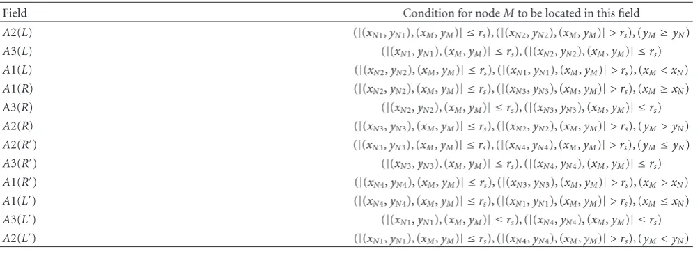
Table2: The conditions for nodeMto be placed in a specific quadrant and field over nodeN’s sensing region.
Field Condition for nodeMto be located in this field
A2(L) (|(xN1,yN1), (xM,yM)| ≤rs), (|(xN2,yN2), (xM,yM)|> rs), (yM≥yN)
A3(L) (|(xN1,yN1), (xM,yM)| ≤rs), (|(xN2,yN2), (xM,yM)| ≤rs)
A1(L) (|(xN2,yN2), (xM,yM)| ≤rs), (|(xN1,yN1), (xM,yM)|> rs), (xM< xN)
A1(R) (|(xN2,yN2), (xM,yM)| ≤rs), (|(xN3,yN3), (xM,yM)|> rs), (xM≥xN)
A3(R) (|(xN2,yN2), (xM,yM)| ≤rs), (|(xN3,yN3), (xM,yM)| ≤rs)
A2(R) (|(xN3,yN3), (xM,yM)| ≤rs), (|(xN2,yN2), (xM,yM)|> rs), (yM> yN)
A2(R) (|(x
N3,yN3), (xM,yM)| ≤rs), (|(xN4,yN4), (xM,yM)|> rs), (yM≤yN)
A3(R) (|(x
N3,yN3), (xM,yM)| ≤rs), (|(xN4,yN4), (xM,yM)| ≤rs)
A1(R) (|(xN4,yN4), (xM,yM)| ≤rs), (|(xN3,yN3), (xM,yM)|> rs), (xM> xN)
A1(L) (|(xN4,yN4), (xM,yM)| ≤rs), (|(xN1,yN1), (xM,yM)|> rs), (xM≤xN)
A3(L) (|(x
N1,yN1), (xM,yM)| ≤rs), (|(xN4,yN4), (xM,yM)| ≤rs)
A2(L) (|(x
N1,yN1), (xM,yM)| ≤rs), (|(xN4,yN4), (xM,yM)|> rs), (yM< yN)
Figure 7(a)shows fieldA3 along with fieldsA1 andA2 which together form the quadrant. Specifically
Area(A1)=Area(A2)=
πr2
s
12 −
πr2
s/6
−r2
s
√ 3/4 2
,
Area(A3)=
πr2
s
4 −2Area(A1)
.
(25)
Figure 7(b)shows these three fields separately for each one of the quadrants where the quadrant name is indicated in parentheses and appended to the field name.
Let us also consider the random placement of more than one neighboring node over the quadrant. In this case, either one of the conditions below satisfies full coverage of the quadrant.
Condition 1. At least one of the neighboring nodes should be located in the fieldA3.
Condition 2. There should be at least one neighboring node in each one of the fieldsA1andA2.
These conditions apply to all quadrants since each one of them has its ownA1,A2, andA3 fields.
We next give an important lemma which describes the coverage relationship between different quadrants of the same sensing region. The key observation here is that the existence of active neighboring nodes in a quadrant can compensate for the uncovered parts of its adjacent quadrants. Two quadrants are referred to as adjacent if they have a common boundary of length rs and they constitute a
contiguous (S/2).
Example 2. The quadrantLis adjacent toLandRbut not
R.
Lemma 2. LetU1 andU2 be the set of active nodes that are
located over the adjacent quadrants Q1 and Q2, respectively,
whereQ1,Q2∈ {L,L,R,R}, andQ1=/Q2. An element ofU1 placed inA1(Q1)field has an equal coverage effect on Q2as compared to an element ofU2placed inA1(Q2). This property is also symmetric and is applicable to A2 fields of adjacent quadrants.
Proof ofLemma 2.The proof is available in the Appendix.
From Lemma 2, Condition 2 for the full coverage of each quadrant is rephrased as follows. Let the neighboring subregions ofSsubbe denoted bySsub,A1andSsub,A2according to the type of adjacent field thatSsubhas with its neighboring quadrant where Ssub,Ssub,A1,Ssub,A2 ∈ {L,L,R,R} and
Ssub=/ Ssub,A1=/ Ssub,A2.
Example 3. IfSsubis equal toLthenSsub,A1=RandSsub,A2=
Lsince the quadrantsLandRhave adjacentA1 fields while quadrantsLandLhave neighboringA2 fields.
Then, for the full coverage ofSsub, Condition2requires the existence of at least one neighboring node in each one of the following fields.
(i)A2(Ssub),A1(Ssub) orA1(Ssub,A1). (ii)A1(Ssub),A2(Ssub) orA2(Ssub,A2).
The remaining question that needs to be answered is how to determine the field and the quadrant that a neighboring is located.
Let us consider a nodeNwith coordinates (xN,yN) which
computes the covered portion of its sensing region. Let node
Mbe one of neighboring nodes of nodeNwith coordinates (xM,yM) where |(xN,yN), (xM,yM)| ≤ rs. Table 2 gives a
set of simple conditions that can be checked by node N
to identify the particular quadrant and field at which node
M is located. In these conditions, if node M is located at the boundary of two quadrants, it is assumed to belong to the right quadrant in clockwise order. The conditions are expressed in terms of distance of node M to the points
Once the exact quadrant and field information for each neighboring node is determined, the sensor node verifies whether each one of its quadrants is covered completely by checking Condition1and Condition2.
We next address the effect of environmental factors on coverage computation. The changes in weather and ground status result in differences between the effective sensing ranges of nodes and theirnominalsensing ranges. To incor-porate effective sensing ranges into coverage computation, CORA considers bothsingle-node detectableandmulti-node detectable environmental factors such as humidity level and rain, respectively. Let β denote the set of all such environmental factors taken into account by the sensor nodes. For each sensing unit, a correction constant Ci is
associated with ith environmental factor fori = 1· · · |β| where −1 ≤ Ci ≤ 1. The magnitude and sign of
each correction constant is determined by experimental evaluation with sensor hardware and different settings for the environmental factor it is associated with. The negative and positive sign for Ci represents the degradation and
improvement in the sensing ability of the sensing unit due to theith environmental factor, respectively, [35].
The effective sensing range of a sensing unitrsis obtained
by adjusting its nominal sensing rangersas
rs=
Once the effective sensing range is determined, it is broadcast to the neighboring nodes at the beginning of each round before the coverage scheduling takes place. In order to check the full coverage of its quadrants, a sensor node compares its distance to each one of its neighboring nodes with its effective sensing range. Then, among those neighboring nodes within the sensing region, the sensor node considers only the ones which have larger effective sensing ranges than itself while checking Condition1and Condition2. For the quadrants that are not fully covered, the coverage of the segments are determined based on the intersection of effective sensing ranges of the node itself and its neighboring node.
5.3.1. Noise in Internode Distance Measurements. The clus-terhead uses the distances between pairs of cluster members to create a local coordinate system. The coordinate assigned to each cluster member is not exact and has an error margin [36]. This section considers how such errors in node location estimates can be incorporated into coverage computation. In the absence of exact node coordinate information, we express coverage and event miss-ratio in terms of expected values rather than absolute values.
Let us represent the maximum deviation on thex and
y coordinates of sensor nodes as Δx andΔy, respectively. A cluster member with coordinate estimates (x,y) may be located at any point within the ellipsis bounded by a box of width (2×Δx) and of height (2×Δy). In what follows, we denote the set of all candidate points for theexactlocation of the node in this ellipsis byR(x,y).
Let us now consider the coverage of any given cluster member Ki’s sensing area by its neighboring nodes where
1≤i≤nK. We refer to nodeKi’s location as (x,y) and the
neighboring nodes that can contribute to the coverage of its sensing region as the setZ. In the case of location errors, we define two sets of angles for the coverage of each segment withinKi’s sensing region. These sets of angles, namely,Ωk
andΩ∗k, represent the worst and best possible cases for the
coverage of thekth segment by the neighboring sensor nodes inZ, respectively, where 1≤k≤nG.
LetKjrepresent one of the neighboring nodes inZwith
coordinates (xj,yj) that covers a part ofkth segment within
nodeKi’s sensing region where 1≤ j ≤nK andi /=j. Now
consider the possible cases for the actual locations of nodes
KiandKjthat minimizes and maximizes the covered part of
the nodeKi’s sensing region by nodeKj, respectively. For the
worst case placement in terms of coverage, let us assume that nodeKj’s coordinates are (xj,yj) and nodeKiis located at
(x,y) where (xj,yj) ∈ R(xj,yj) and (x,y) ∈ R(x,y).
Similarly, also assume that when node Kj is positioned at
(x∗j,y∗j) andKi has coordinates (x∗,y∗), the best case for best case contribution of node Kj for the coverage of the
kth segment, respectively. Ωk and Ω∗k are updated with
the addition of ρ andρ∗, respectively. The same coverage computation is applied for each neighboring node in setZ
in addition to node Kj. Once the coverage contribution of
all neighboring nodes is determined, we defineE(Ck) as the
expectedcovered portion ofkth segment where
E(Ck)=
andΣ(Ω) represents the sum of the magnitudes of angles in a set Ω. From the coverage of each segmentk for 1 ≤
300 250 200 150 100
Number of nodes in the network γreq=0.3
(a) CORA takes advantage of the increase in network population and the required event miss-ratio thresholds to reduce the number of events to be sensed by each node
0.5 0.4 0.3 0.2 0.1
Required event miss-ratioγreq 0.05
(b) The experimental validation of the event miss-ratio assurances
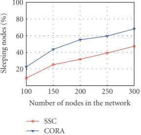
Number of nodes in the network SSC
(c) CORA uses less number of active nodes to meet a given coverage requirement than the sponsored sector based coverage (SSC) scheduling technique proposed in [5]
Figure8: Performance evaluation of coverage scheduling.
is determined as
CORA is evaluated in terms of event miss-ratios, total energy expenditure, average node battery consumption, and the storage/update overhead for the application of source coding. In the simulations, we consider sensor networks with multiple clusters in which the clusters are formed based on residual energy of sensor nodes. Each network is simulated for a single round with 100 data gatherings. For uniform event distribution, every sensor node within a cluster is assumed to detect an event per data gathering. For nonuniform event distribution, we have randomly selected hotspot centers. At each data gathering, the event occur-rences are modeled around these hotspot centers following the Gaussian distribution.
In the simulation graphs, the results for uniform and nonuniform event distributions are illustrated with solid and dashed lines, respectively. Each point shown in the graphs is obtained by averaging the simulation outcomes from a large number sensor networks. The sensor networks are deployed randomly over a target area of side length 100 m. The number of sensor nodes in each network is selected from the interval [100–300] to control node/coverage redundancy. As network population increases, the sensing ranges of nodes overlap more, thereby increasing both the number of nodes redundant for coverage and the data correlation among neighboring sensor nodes.
The sensing range and transmission range of the nodes are set to 10 m and 30 m, respectively. The initial residual energy level of each node is assigned as 10 Joules. To calculate the energy expenditure, we have used the radio power consumption model described inSection 3with settingsa= 0.01 andb = 0.03. The entropy of the source at a single cluster member is modeled as nB = 16 bits. The ratio of
the control message size to the data message size is set to
ε=0.2. Unless specified otherwise, the required event miss-ratio threshold is equal to 0.2.
Figure 8(a)shows the results of the experiments in which we’ve considered sensor nodes equipped with four sensing units for event types Mj, 1 ≤ j ≤ 4. CORA exploits
the increase in node redundancy and required event miss-ratio thresholds to minimize the average number of events scheduled to each sensor node. As simulation results indicate, CORA enables a node to keep only one of its sensing units active at any time with sufficient node redundancy. It is possible that a node keeps its sensing unit active for event typeMiwhile its neighboring node might activate the sensing
unit for a different event type Mk, 1 ≤ i,k ≤ 4,i /=k.
Meanwhile, CORA’s distributed coverage scheduling ensures that event miss-ratio assurances are met for every event types
MiandMk.
Figure 8(b) illustrates the empirical verification of the assurances provided by CORA under different event miss-ratio requirements. For a particular γreq value, a large number of simulations are run while keeping the network population constant. The observed event miss-ratios γobs (shown in y axis ofFigure 8(b)) always remain below the required event miss-ratios γreq (illustrated in x axis of Figure 8(b)).
CORA assigns rates to the active nodes only and therefore is highly scalable. Figure 8(c) shows the results of the simulations that are run with the same required event miss-ratio value but with varying number of nodes. Even though the network population increases, CORA limits the number of nodes that are scheduled active and get assigned rates. Having only a smaller set of nodes active prolong the time event miss-ratio assurances can be met as those sensor nodes which are put in off-duty mode can save their energy to go active in the subsequent scheduling phases.