R E S E A R C H
Open Access
A fast implicit difference scheme for a new
class of time distributed-order and space
fractional diffusion equations with variable
coefficients
Huan-Yan Jian
1*, Ting-Zhu Huang
1, Xi-Le Zhao
1and Yong-Liang Zhao
1*Correspondence:
1School of Mathematical Sciences, University of Electronic Science and Technology of China, Chengdu, P.R. China
Abstract
Recently, several problems in mathematics, physics, and engineering have been modeled via distributed-order fractional diffusion equations. In this paper, a new class of time distributed-order and space fractional diffusion equations with variable coefficients on bounded domains and Dirichlet boundary conditions is considered. By performing numerical integration we transform the time distributed-order fractional diffusion equations into multiterm time-space fractional diffusion equations. An implicit difference scheme for the multiterm time-space fractional diffusion equations is proposed along with a discussion about the unconditional stability and convergence. Then, the fast Krylov subspace methods with suitable circulant preconditioners are developed to solve the resultant linear system in light of their Toeplitz-like structures. The aforementioned methods are proved to acquire the capability to reduce the memory storage of the proposed implicit difference scheme fromO(M2) toO(M) and the computational cost fromO(M3) toO(MlogM) during iteration procedures, whereMis the number of grid nodes. Finally, numerical experiments are employed to support the theoretical findings and show the efficiency of the proposed methods.
MSC: 26A33; 65F08; 65M06
Keywords: Multi-term time-space fractional diffusion; Distributed-order fractional derivative; Shifted Grünwald discretization; Toeplitz matrix; Circulant preconditioner; Krylov subspace method
1 Introduction
In the past few decades, the fractional calculus has attracted considerable attention and interest due to its extensive applications in modeling practical scientific problems, such as heat-transfer engineering [1], anomalous relaxation models [2], solid mechanics [3], vis-coelastic materials [4], continuum and statistical mechanics [5], mathematical physics [6], control system [7], chaos [8,9], finance [10], electromagnetics [11,12], and image process-ing [13]. Based on different problems, a variety of fractional diffusion equations (FDEs) need to be solved, in which the time-fractional anomalous FDE is always an important concern of many mathematicians; refer, e.g., to [14–16] and references therein.
However, some complex physical processes [17, 18] that lack temporal scaling over the whole time domain cannot be described by the time-fractional anomalous FDEs with a constant-order temporal derivative. Such processes can be modeled via the time distributed-order FDEs. The idea of distributed-order FDE was first proposed by Ca-puto (see [19] and references therein). Chechkin et al. [20] presented diffusion-like equa-tions with time and space fractional derivatives of distributed order for the kinetic de-scription of anomalous diffusion and relaxation phenomena, and showed that the time distributed-order FDE can describe the accelerating superdiffusion and retarding subdif-fusion. Boundary value problems for the generalized time-FDE of distributed order over an open bounded domain were considered by Luchko [21]. Furthermore, Meerschaert et al. [22] gave explicit strong solutions and stochastic analogues to time distributed-order FDE on bounded domains, with Dirichlet boundary conditions. By employing the tech-niques of the Fourier and Laplace transforms, a fundamental solution to the Cauchy prob-lem for the distributed-order time-fractional diffusion-wave equation in the transform do-main was obtained by Gorenflo et al. [23]. Jiang et al. [24] derived the analytical solutions of multiterm time-space Caputo–Riesz fractional advection diffusion equations with Dirich-let nonhomogeneous boundary conditions. For more general distributed-order FDEs, the analytical solutions are not easily acquired. Therefore, numerical methods are worth con-sidering to solve the distributed-order FDEs.
In a more general sense, the first step is to approximate the distributed integral with a finite sum based on a simple quadrature rule when solving distributed-order FDEs via nu-merical methods. Thus the distributed-order FDE is converted into a multiterm FDE [25], and we have to efficiently solve the approximated multiterm FDE. To our knowledge, only a few articles have considered such problem. Liu et al. [26] discussed some computationally effective numerical methods for simulating the multiterm time-fractional wave-diffusion equations and extended such numerical techniques to other kinds of multiterm fractional time-space models with fractional Laplacian operator. Morgado et al. [27] studied a nu-merical approximation for the time distributed-order FDE concerning the stability and convergence; they [28] also presented an implicit difference scheme for numerical approx-imation of the distributed-order time fractional reaction–diffusion equation with nonlin-ear source term. An implicit difference scheme for the time distributed-order and Riesz space FDE on bounded domains with Dirichlet boundary conditions was constructed by Ye et al. [29]. Mashayekhi et al. [30] introduced a new numerical method for solving the distributed-order FDEs, which is based upon hybrid functions approximation. Hu et al. [31] provided an implicit numerical method of a new time distributed-order and two-sided space fractional advection–dispersion equation and proved the uniqueness, stability, and convergence of the method. A numerical method of distributed-order FDEs of a general form was investigated by Katsikadelis [25], where the trapezoidal rule was employed to ap-proximate the distributed integral, and the analog equation method was applied to solve the resultant multiterm FDE. However, the stability and convergence were only shown in the experimental examples, and there was no rigorous theoretical proof.
in particular a fast and stable numerical approach for solving the following new class of time distributed-order and space FDEs (TDFDEs) with variable coefficients and initial boundary conditions:
Dωt(α)u(x,t) =d+(x,t)RLDβ0,xu(x,t) +d–(x,t)RLDx,Lβ u(x,t) +f(x,t),
0 <x<L, 0 <t≤T, (1.1)
u(0,t) = 0, u(L,t) = 0, 0≤t≤T, (1.2)
u(x, 0) =ψ(x), 0≤x≤L, (1.3)
where α∈[0, 1],β ∈(1, 2),x∈[0,L],t∈[0,T], andf(x,t),d±(x,t), andψ(x) are given functions. Here f(x,t) is the source term, and diffusion coefficient functions d±(x,t)
are nonnegative, that is,d±(x,t)≥0. Specifically, the time fractional derivativeDωt(α) of
distributed-order is denoted by [21]
Dωt(α)u(x,t) =
1
0
ω(α)C0Dtαu(x,t)dα
with the left-handed Caputo fractional derivativeC
0Dαt defined as [34,35]
C
0Dαtu(x,t) =
⎧ ⎨ ⎩
1
(1–α)
t 0(t–ξ)–
α ∂u
∂ξ(x,ξ)dξ, 0≤α< 1,
ut(x,t), α= 1,
and a continuous nonnegative weight function ω(α) on the interval [0, 1] such that 1
0 ω(α)dα =c0 > 0. Moreover, RLD
β
0,x and RLDβx,L are the the left- and right-handed
Riemann–Liouville fractional derivatives of orderβ∈(1, 2) [36,37] defined respectively as
RLDβ0,xu(x,t) =
1 (2 –β)
∂2 ∂x2
x
0
u(ξ,t) (x–ξ)β–1dξ
and
RLD
β
x,Lu(x,t) =
1 (2 –β)
∂2
∂x2
L
x
u(ξ,t) (ξ–x)β–1dξ,
where(·) denotes the gamma function.
Since the fractional differential operator is nonlocal [38,39], a naive discretization of the FDE leads to traditional approaches [40] of solving FDEs, which tend to generate dense systems, whose solution with Gaussian elimination costsO(M3) arithmetic operations
and requires a storage of orderO(M2). Wang and Wang [41] found that the coefficient
matrix had a Toeplitz structure in the linear system, which was generated by the dis-cretization introduced in [42]. More precisely, this coefficient matrix can be expressed as a sum of diagonal-multiply-Toeplitz matrices. This implied that the storage require-ment wasO(M) instead ofO(M2), and the complexity of the matrix–vector
(CGNR) method to solve the discretized linear systems inO(Mlog2M) arithmetic oper-ations. The convergence of the CGNR method can be fast when the diffusion coefficients are very small, that is, discretized systems are well-conditioned [44]. Nevertheless, if the diffusion coefficient functions are not small, the resultant systems become ill-conditioned, and hence the CGNR method converges very slowly.
To overtake this shortcoming and get a faster convergence, some Krylov subspace meth-ods with circulant preconditioners have been studied and extended. Lei and Sun [45] de-veloped the preconditioned CGNR (PCGNR) method with a circulant preconditioner, an extension of the Strang circulant preconditioner [46], to solve the discretized Toeplitz-like linear systems of the FDE. Pan et al. [47] introduced approximate inverse precondi-tioners for such systems and proved that the spectra of the preconditioned matrices are clustered around one. Thus Krylov subspace methods with the proposed preconditioner converge very fast. Donatelli et al. [48] proposed two tridiagonal structure-reserving pre-conditioners with CGNR and generalized minimal residual (GMRES) methods for solving the resultant Toeplitz-like linear systems. Using the short-memory principle [49] to gen-erate a sequence of approximations for the inverse of the discretization matrix with a low computational effort, Bertaccini et al. [50] solved the mixed classical and fractional partial differential equations effectively by preconditioned Krylov iterative methods. Our recent work [51] showed that the preconditioned conjugate gradient squared (PCGS) method with suitable circulant preconditioners can efficiently solve the resultant Toeplitz-like lin-ear systems.
In this paper, we focus on deriving a fast implicit difference scheme for solving the new problem (1.1)–(1.3). We first transform TDFDEs into multiterm time-space FDEs by ap-plying numerical integration. Then we present an implicit difference scheme with uncon-ditional stability and convergence that is first-order accurate in space and (1 + σ2)-order accurate in time. We prove these properties of the proposed scheme both theoretically and numerically. On the other hand, we show that the discretizations of TDFDEs lead to a nonsymmetric Toeplitz-like system of linear equations. The linear system can be solved efficiently by using Krylov subspace methods with suitable circulant preconditioners [52– 54]. It can greatly reduce the memory and computational costs; the memory requirement and computational complexity are onlyO(M) andO(MlogM) in each iteration step, re-spectively. Meanwhile, it is meaningful to investigate the performance of some other pre-conditioned Krylov subspace solvers, such as the prepre-conditioned biconjugate gradient stabilized (PBiCGSTAB) method [55], the preconditioned biconjugate residual stabilized (PBiCRSTAB) method [56], and the preconditioned GPBiCOR(m,) (PGPBiCOR(m,)) method [57].
The rest of this paper is organized as follows. In Sect.2, we present an implicit difference scheme for the TDFDEs. The uniqueness, unconditional stability, and convergence of the implicit difference scheme are analyzed in Sect.3. In Sect.4, we show that the resultant linear system has nonsymmetric Toeplitz matrices and design fast solution techniques based on preconditioned Krylov subspace methods to solve problem (1.1)–(1.3). In Sect.5, we present numerical experiments to show the effectiveness of the numerical method. Concluding remarks are given in Sect.6.
2 An implicit difference scheme for TDFDEs
us-ing numerical integration, and we show that the discretizations lead to multiterm time-space FDEs. Then we propose an implicit difference scheme with the shifted Grünwald– Letnikov formulae approximation to solve the mutiterm time-space FDEs.
For simplicity, but without loss of the generality, we first divide the integral interval [0, 1] intoq-subintervals with 0 =ξ0<ξ1<ξ2<· · ·<ξq= 1 and takeξs=ξs–ξs–1=1q =σ (q∈
N),αs=ξs–12+ξs=2s–12q (s= 1, 2, . . . ,q). The following lemma gives a complete description of
the discretization in the integral term.
Lemma 2.1(The compound midpoint quadrature rule [29]) Let z(α)∈C2[0, 1],α= 1/q=σ(q∈N).Then we have
1
0
z(α)dα=
q
s=1
z
2s– 1
2q
1
q+O
σ2.
Considering the left side of formula (1.1), let z(α) =ω(α)C0Dα
tu(x,t) and suppose that
ω(α)∈C2[0, 1] andC
0Dαtu(x,t)∈C2[0, 1]. Using Lemma2.1, we obtain
Dωt(α)u(x,t) = q
s=1
ds
C
0D
αs t u(x,t)
+Oσ2, (2.1)
whereds=ω(αs)ξs. Thus problem (1.1)–(1.3) is now transformed into the following
mul-titerm time-space FDEs:
q
s=1
ds
C
0D
αs t u(x,t)
=d+(x,t)RLDβ0,xu(x,t) +d–(x,t)RLDβx,Lu(x,t) +f(x,t),
0 <x<L, 0 <t≤T, (2.2)
u(0,t) = 0, u(L,t) = 0, 0≤t≤T, (2.3)
u(x, 0) =ψ(x), 0≤x≤L. (2.4)
Next, we solve the multiterm time-space FDEs. We discretize the domain [0,L]×[0,T] withxi=ih,i= 0, 1, 2, . . . ,M, andtk=kτ,k= 0, 1, 2, . . . ,N, whereh=ML andτ=TN are the
sizes of spatial grid and time step, respectively.
The following two lemmas will be further useful in the discretizations of the multiterm time-space FDEs.
Lemma 2.2([58]) Let0 <α< 1,and let u be absolutely continuous in t on [0,T]with
∂2u/∂t2∈C([0,L]×[0,t
k]).Then
C 0D
α
tu(x,tk) =
1 μ
u(x,tk) – k–1
j=1
aαk–j–1–aαk–ju(x,tj) –aαk–1u(x,t0)
+Oτ2–α,
where aα
k= (k+ 1)1–
α–k1–α,μ=τα(2 –α), 0≤t
k≤T.
Lemma 2.3 ([59]) For 1 <β < 2,suppose that u ∈L1(R)∩Cβ+1(R). Then the shifted
deriva-tives as follows:
where g(jβ)is the alternating fractional binomial coefficient given as
⎧
the Caputo time-fractional derivative forαs∈(0, 1) can be approximated by
C
By Lemma2.3the left and right Riemann–Liouville derivatives of orderβ∈(1, 2) can be approximated by adopting the shifted Grünwald–Letnikov formula as follows:
RLD
Applying formulae (2.5)–(2.7) to equation (2.2), by (2.1) we obtain
q where there exists a positive constantκ1such that
pk+1i =Oh+τ1+σ/2+σ2≤κ1
Letuki be a numerical approximation toUik. By omitting the local truncation error term
pk+1
i in (2.8) and considering the discretization of the initial and boundary conditions
(1.2)–(1.3) we obtain the following implicit difference scheme for TDFDEs (1.1)–(1.3):
q
For convenience of the following theoretical analysis, we define
v= h
Thus, we rewrite the difference scheme (2.10)–(2.12) as follows:
withDk+1
± =diag(dk+1±,1, . . . ,dk+1±,M–1) and
Gβ= ⎡ ⎢ ⎢ ⎢ ⎢ ⎢ ⎢ ⎢ ⎢ ⎢ ⎣
g1(β) g0(β) 0 · · · 0 0
g2(β) g1(β) g0(β) · · · 0 0
g3(β) g2(β) g1(β) · · · 0 0 ..
. ... ... . .. ... ...
gM–2(β) g(M–3β) gM–4(β) · · · g(1β) g0(β) gM–1(β) g(M–2β) gM–3(β) · · · g(2β) g1(β)
⎤ ⎥ ⎥ ⎥ ⎥ ⎥ ⎥ ⎥ ⎥ ⎥ ⎦ .
It is obvious thatGβis a Toeplitz matrix (see [46]). Furthermore, the linear system (2.17) can be written as
Mk+1uk+1=bk, k= 0, 1, 2, . . . ,N– 1, (2.18)
where
Mk+1=I–vAk+1=I–vDk+1+ Gβ+Dk+1– GTβ
and
bk=
k
j=1
ck,juj+bku0+vf¯ k+1.
3 Solvability, stability, and convergence results
In this section, we analyze the unique solvability, unconditional stability, and conver-gence of the implicit difference scheme (2.14)–(2.16). Meanwhile, the difference scheme is proved to converge with the first-order in space and the (1 +σ2)-order in time.
Before proving the most important result of this section on the solvability, stability, and convergence properties, we first need to recall the following useful proposition.
Proposition 3.1([60]) Let1 <β< 2and gj(β)be defined as in Lemma2.3.Then we have
⎧ ⎪ ⎪ ⎨ ⎪ ⎪ ⎩
g0(β)= 1, g1(β)= –β< 0, g(2β)>g3(β)>· · ·> 0, ∞
j=0g (β) j = 0,
m j=0g
(β)
j < 0, m≥1,
gj(β)= (1 –β+1j )gj–1(β), j= 1, 2, 3, . . . .
The starting point of our analysis is the following theoretical result.
Proof Letmk+1ij be the (i,j) entry of the Mk+1 in (2.18). Sincev> 0 and d
±(x,t)≥0, by
Proposition3.1we get
mk+1ii –
M–1
j=1,j=i
mk+1ij =1 –vd+,ik+1+dk+1–,i g1(β)
–v
dk+1+,i
i
j=0,j=1
gj(β)+dk+1–,i
M–i
j=0,j=1
gj(β)
≥1 –vdk+1+,i +dk+1–,i g1(β)–vdk+1+,i +d–,ik+1
∞
j=0,j=1
gj(β)
= 1 –vdk+1+,i +dk+1–,i
∞
j=0
gj(β)= 1 > 0.
This implies that the coefficient matrixMk+1is a strictly diagonally dominant M-matrix
(see [41]), and therefore it is nonsingular, so the difference scheme (2.14)–(2.16) is uniquely
solvable.
The unique solvability of the implicit difference scheme (2.14)–(2.16) has been estab-lished, and now we further show its stability.
Theorem 3.3 The difference scheme(2.14)–(2.16)for the TDFDEs is unconditionally sta-ble,where1 <β< 2.
Proof Assume that the initial errors areεi0(i= 0, 1, . . . ,M– 1), letψ¯i0=ψi0+εi0, and letuki
andu¯k
i be the numerical solutions of scheme (2.14) corresponding to the initial dataψi0
andψ¯0
i (i= 1, 2, . . . ,M– 1), respectively. Thenεik=uki –u¯ki satisfies
ε1i –v
d+,i1
i+1
j=0
gj(β)ε1i–j+1+d1–,i
M–i+1
j=0
g(jβ)ε1i+j–1
=
q
s=1
vsaα0sεi0=ε0i,
εk+1i –v
dk+1+,i
i+1
j=0
gj(β)εk+1i–j+1+dk+1–,i
M–i+1
j=0
g(jβ)εk+1i+j–1
=
k
j=1
q
s=1
vs
aαs k–j–a
αs k–j+1
εji+
q
s=1
vsaαksε0i, k= 1, . . . ,N– 1.
DenoteEk= [εk
1,εk2, . . . ,εkM–1]T. The theorem will be proved if we show that
Ek+1∞≤E0∞, k= 0, 1, 2, . . . .
For k= 0, denote |ε1
≤εk+1l –v
which completes the proof of Theorem3.3.
The next step is to analyze the convergence of the implicit method given in (2.14)– (2.16). To this end, suppose that the continuous problem (1.1)–(1.3) has a smooth so-lutionu(x,t)∈Cx,tβ+1,2([0,L]×[0,T]). Recall thatUdenotes the exact solution of system (1.1)–(1.3);urepresents the numerical solution of the implicit difference approximation (2.14)–(2.16) for 1 <β< 2. Let us assume that the errore=U–uat mesh points (xi,tk) is
defined byek
i =Uik–uik(i= 1, 2, . . . ,M– 1;k= 0, 1, 2, . . . ,N). LetRk= [ek1,ek2, . . . ,ekM–1]Tand
R0= [e0
1,e02, . . . ,e0M–1]T= 0.
According to (2.13), equation (2.8) can be rewritten as
Uik+1–v
Subtracting (3.1) from (2.14), we have
ek+1i –v
Theorem 3.4 Suppose that the continuous problem (1.1)–(1.3) has a smooth solution
Suppose that the result is valid for some integerk≥1, that is, Rj∞≤κ1
(2.13), and (3.2), since the coefficientsaαs
+κ1v¯
which proves the theorem.
4 Fast solution techniques based on preconditioned Krylov subspace solvers In this section, we analyze both the implementation and the computational complexity of the implicit difference scheme (2.14)–(2.16) and propose an efficient implementation based on Krylov subspace solvers with suitable circulant preconditioners.
According to (2.17) and (2.18), there is a sequence of nonsymmetric Toeplitz linear sys-tem to be solved at each time levelk. If a direct method is employed to solve the linear system (2.18), the LU decomposition can be reused in each time levelk. This approach, however, needs the memory requirement ofO(M2) and the complexity ofO(M3) per iter-ation step, which is prohibitively expensive ifMis large. Fortunately, sinceGβis a Toeplitz matrix, it can be stored with onlyMentries [41]. The Krylov subspace methods with cir-culant preconditioners [45,61] can be used to solve Toeplitz-like linear systems with a fast convergence rate. In this case, we also remark that the computational complexity of preconditioned Krylov subspace methods is only in O(MlogM) at each iteration step for implementing the implicit difference scheme. In this study, we employ four precon-ditioned Krylov subspace methods, the PBiCGSTAB method, the PBiCRSTAB method, the PGPBiCOR(m,) method, and the PCGNR method. The numerical results show the performance of three proposed preconditioned Krylov subspace solvers over the LU de-composition and the PCGNR method, while solving (2.18), and reveal that the results of the PGPBiCOR(m,) method are better than others whenm= 2,= 1.
The PGPBiCOR(2,1) method with the preconditionerKapplied to the systemAx=bis given in Algorithm4.1.
Now we propose a circulant preconditioner generated from the Strang circulant precon-ditioner [46] in the PGPBiCOR(2,1) method for solving (2.18). For a real Toeplitz matrix
Q= [qj–m]0≤j,m<N, the Strang circulant matrixs(Q) = [sj–m]0≤j,m<N is obtained by copying
Algorithm 4.1PGPBiCOR(2,1) forAx= b with preconditionerK conditioner is defined as
Sk+1=I–vd¯+k+1s(Gβ) +d¯k+1– sGTβ
of variable diffusion coefficients. We further show that the preconditionerSk+1defined
in (4.1) is also nonsingular and thus is well-defined. Before that, we need the following lemma, which is essential to prove the nonsingularity ofSk+1in (4.1).
Lemma 4.2 All eigenvalues of s(Gβ)and s(GTβ)fall inside the open disc &
z∈C:|z+β|<β'.
Proof All Gershgorin discs [51] of the circulant matricess(Gβ) ands(GT
β) are centered at
g1(β)= –βwith radius
rN=g(
β)
0 +
M 2
j=2
gj(β)<
∞
j=0,j=1
gj(β)= –g1(β)=β
by the properties of the sequence{gj(β)}; refer to Proposition3.1.
Remark4.3 It is worth mentioning that the real parts of all eigenvalues ofs(Gβ) ands(GT
β) are strictly negative for allM.
As we know, a circulant matrixEcan be diagonalized by the Fourier matrixF[43], that is,
E=F∗F,
where the entries ofFare given by
Fj,m=
1 √
Ne
2πijm/N, 0≤j,m≤N– 1,
with the imaginary uniti, andis a diagonal matrix holding the eigenvalues ofE. Then it follows thats(Gβ) =F∗βFands(GTβ) =F∗¯βF, where¯βis the complex con-jugate of β. Decompose the circulant matrixSk+1 =F∗
sF with the diagonal matrix
s=I–v[d¯k+1+ β+d¯k+1– ¯β]. ThenSk+1is invertible if all diagonal entries ofsare nonzero.
Moreover, we can obtain the following conclusion about the invertibility ofSk+1in (4.1).
Theorem 4.4 For1 <β< 2,the preconditioner Sk+1defined as in(4.1)is nonsingular,and
Sk+1–12≤1.
Proof By Remark4.3we haveRe([β]i,i) < 0. Noting thatv> 0 andd¯k+1± ≥0, we obtain
[s]i,i≥Re
[s]i,i
= 1 –vd¯+k+1Re[β]i,i
+d¯k+1– Re[¯β]i,i
≥1 > 0
for eachi= 1, . . . ,M– 1. Therefore,Sk+1is nonsingular. Furthermore, we have Sk+1–12= 1
min1≤i≤M–1|[s]i,i|≤
1.
Unfortunately, when the diffusion coefficientsd±(x,t) are nonconstant functions, the
preconditioned sequence (Sk+1)–1Mk+1cannot be clustered at 1; we refer to [48] for de-tails of the theoretical analysis. For clarity, we still give some figures to illustrate the clus-tering eigenvalue distributions of several specified preconditioned matrices in the next section.
5 Numerical examples
The numerical experiments presented in this section have a two-fold objective. They il-lustrate that the proposed finite difference scheme can indeed converge with first-order in space and (1 +σ
2)-order in time. At the same time, they assess the computational efficiency
of the fast solution techniques (Algorithm4.1) designed in Sect.4. The nonsymmetric linear system (2.18) is solved at each time step by the PCGNR method, the PBiCRSTAB method, the PBiCGSTAB method, the PGPBiCOR(2,1) method (Algorithm4.1), and LU factorization of MATLAB, respectively. The numbers of iterations required for conver-gence and CPU times of those methods are shown further. The stopping criterion of those methods is
r(k)2
r(0) 2
< 10–12,
wherer(k)is the residual vector of the linear system afterkiterations, and the initial guess is
chosen as a zero vector. In the following tables, settinge(h,τ,σ) =max1≤i≤M–1|u(xi,tN,σ)–
uNi |, whereu(xi,tN,σ) id the exact solution, anduNi is the numerical solution with step sizes
handτ attN=T. The convergence order is computed by
rateh=log2
e(h,τ,σ)
e(h/2,τ,σ),
rateτ =log2
e(h,τ,σ)
e(h,τ/2,σ),
rateσ =log2
e(h,τ,σ)
e(h,τ,σ/2).
The number of spatial grid points is denoted byM,Ndenotes the number of time steps, CPU (s) denotes the total CPU time in seconds for solving the whole TDFDEs problem, and Iter denotes the average number of iterations required for solving the TDFDEs prob-lem, that is,
Iter = 1
N
N
n=1
Iter(n),
where Iter(n) denotes the number of iterations required for solving (2.18). For those meth-ods, besides the proposed circulant preconditionerSk+1in (4.1), we also test the T. Chan’s
preconditioner [43] which can be written as
cMk+1=I–vd¯+k+1c(Gβ) +d¯k+1– c
GTβ
wherec(Q) denotes Chan’s preconditioner for an arbitrary matrixQ. More specifically, the
In all tables, the symbols “PCGNR(S)”, “PBiCRSTAB(S)”, “PBiCGSTAB(S)”, and “PGPBi-COR(S)” correspond to the PCGNR, PBiCRSTAB, PBiCGSTAB, and PGPBiCOR methods with the circulant preconditionerSk+1, respectively. Similarly, the symbols “PCGNR(C)”, “PBiCRSTAB(C)”, “PBiCGSTAB(C)”, and “PGPBiCOR(C)” denote Chan’s circulant pre-conditioner c(Mk+1) for the PCGNR, PBiCRSTAB, PBiCGSTAB, and PGPBiCOR(2,1)
methods, respectively. All numerical experiments are implemented in MATLAB (R2013a) on a desktop PC with 4 GB RAM, Inter (R) Core (TM) i3-2130 CPU, @3.40 GHz.
Example5.1 Consider the following time distributed-order and space fractional diffusion equations with variable coefficients:
⎧
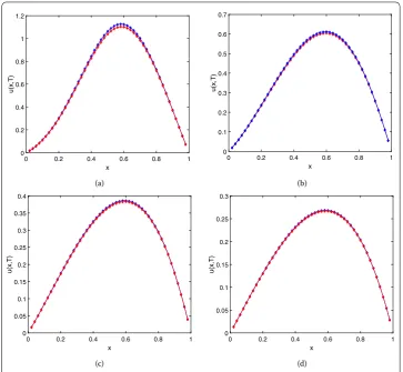
The errors and convergence orders are displayed in Tables1and2. We can clearly see that the convergence orders are of first-order in space and (1 +σ
2)-order in time, which
verifies the correctness of our theoretical results.
Table 1 Maximum errors and spatial convergence orders of difference scheme (2.14)–(2.16) for Example5.1withα= 0.5;σ= 0.1;T= 1.5;N= 800
M β= 1.3 β= 1.5 β= 1.8
e(h,τ,σ) rateh e(h,τ,σ) rateh e(h,τ,σ) rateh
20 3.978980e–03 – 1.594856e–03 – 9.815094e–04 –
40 2.181749e–03 0.8669 8.201275e–04 0.9595 3.974269e–04 1.3043
80 1.144519e–03 0.9307 4.133978e–04 0.9883 1.779229e–04 1.1594
160 5.855271e–04 0.9669 2.080332e–04 0.9907 8.429100e–05 1.0778 320 2.950680e–04 0.9887 1.046050e–04 0.9919 4.121610e–05 1.0322
Table 2 Maximum errors and temporal convergence orders of difference scheme (2.14)–(2.16) for Example5.1withα= 0.5;σ= 0.2;T= 1.5;M= 2000
N β= 1.3 β= 1.5 β= 1.8
e(h,τ,σ) rateτ e(h,τ,σ) rateτ e(h,τ,σ) rateτ
5 6.897311e–04 – 4.256675e–04 – 2.559967e–04 –
10 2.640520e–04 1.3852 1.711099e–04 1.3148 1.099115e–04 1.2198
20 8.702462e–05 1.6013 6.546150e–05 1.3862 4.935518e–05 1.1551
40 4.570569e–05 0.9290 3.003826e–05 1.1238 2.399388e–05 1.0405
Figure 1Exact solutions (lines) and numerical solutions (symbols) of Example5.1withβ= 1.8 att= 0.3 (rounds),t= 0.75 (squares),t= 1.5 (rhombus)
In Figs.2and3, the eigenvalue plots of the original matrixMk+1and the preconditioned matrices (Sk+1)–1Mk+1are plotted. These two figures confirm that the circulant precon-ditioning exhibits very nice clustering properties. The eigenvalues of preconditioned ma-trices are clustered at 1, except for a few outliers. It indicates that the vast majority of the eigenvalues are well separated away from 0. It may guarantee that our proposed precon-ditioners can deeply accelerate Krylov subspace methods for solving the nonsymmetric Toeplitz system. We also validate the effectiveness and robustness of the designed circu-lant preconditioner from the perspective of clustering spectrum distribution.
(a) (b)
Figure 2Spectrum of original matrix (red) and preconditioned matrix (blue) for Example5.1at time level (a):k= 0 and (b):k= 1, respectively, whenM=N= 128,α= 0.5,q= 10,β= 1.8, andT= 0.75
(a) (b)
Figure 3Spectrum of original matrix (red) and preconditioned matrix (blue) for Example5.1at time level (a):k= 0 and (b):k= 1, respectively, whenM=N= 256,α= 0.5,q= 10,β= 1.8, andT= 1.5
Example5.2 Consider the following equation: ⎧
⎪ ⎪ ⎪ ⎪ ⎪ ⎨ ⎪ ⎪ ⎪ ⎪ ⎪ ⎩
1
0ω(α)C0Dtαu(x,t)dα
=d+(x,t)RLD0,xβ u(x,t) +d–(x,t)RLDβx,Lu(x,t) + (1 +t2)sinx, 0 <x< 1, 0 <t≤5,
u(0,t) = 0, u(1,t) = 0, 0≤t≤5,
u(x, 0) = 10δ(x), 0≤x≤1,
where 1 <β≤2,d+(x,t) = (1 +t)x0.6,d–(x,t) = (1 +t)(1 –x)0.6.
Table 3 Comparisons for solving Example5.1by the LU method and the PCGNR/PBiCRSTAB method with two circulant preconditioners, whereβ= 1.3, 1.5, 1.8,α= 0.5,q= 10, andT= 0.75
β M N LU PCGNR(S) PCGNR(C) PBiCRSTAB(S) PBiCRSTAB(C)
CPU(s) CPU(s) Iter CPU(s) Iter CPU(s) Iter CPU(s) Iter
1.3 26 22 0.01 0.02 18.0 0.01 16.8 0.02 14.0 0.02 14.0
27 23 0.01 0.04 20.0 0.04 20.4 0.04 18.6 0.04 18.9
28 24 0.13 0.09 22.9 0.09 24.8 0.11 22.3 0.10 21.7
29 25 1.36 0.38 25.4 0.44 30.2 0.45 26.3 0.42 25.3
210 26 16.72 1.20 27.5 1.72 40.9 1.47 30.5 1.39 29.0
211 27 213.81 7.99 28.8 16.74 63.1 9.60 33.5 16.23 58.7
1.5 26 22 0.01 0.03 18.0 0.03 14.0 0.01 12.0 0.01 11.8
27 23 0.01 0.03 19.3 0.03 17.0 0.03 14.0 0.03 14.0
28 24 0.14 0.08 21.8 0.08 19.2 0.08 16.4 0.08 16.0
29 25 1.40 0.34 23.3 0.32 21.6 0.32 18.4 0.32 18.7
210 26 16.86 1.05 24.1 1.06 24.2 1.01 20.6 1.00 20.3
211 27 217.19 6.69 24.2 7.20 25.9 6.16 21.3 6.34 22.0
1.8 26 22 0.01 0.04 18.5 0.03 16.0 0.01 8.0 0.01 9.0
27 23 0.01 0.04 22.0 0.03 18.8 0.02 9.0 0.03 10.6
28 24 0.14 0.09 24.0 0.09 22.9 0.06 10.0 0.07 12.8
29 25 1.43 0.36 26.1 0.41 27.8 0.21 11.0 0.26 14.9
210 26 17.16 1.21 27.3 1.47 34.4 0.61 11.0 0.86 17.0
211 27 221.05 8.22 29.7 12.02 44.7 3.66 11.6 5.86 20.0
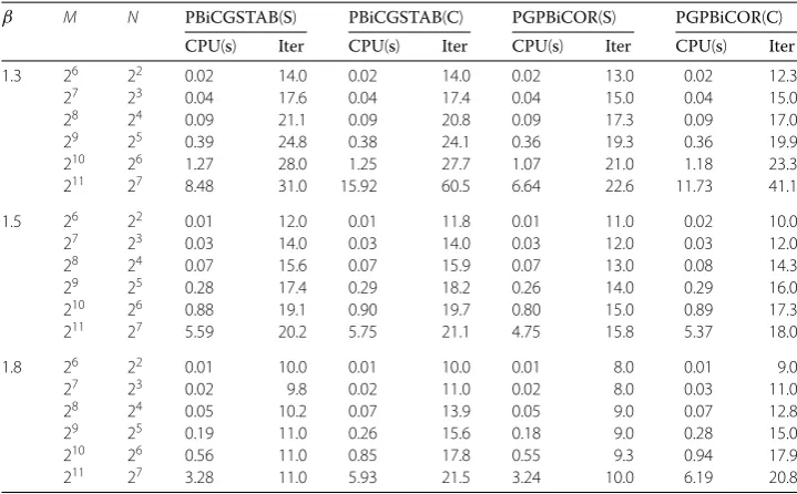
Table 4 Comparisons for solving Example5.1by the PBiCGSTAB/PGPBiCOR(2, 1) method with two circulant preconditioners, whereβ= 1.3, 1.5, 1.8,α= 0.5,q= 10, andT= 0.75
β M N PBiCGSTAB(S) PBiCGSTAB(C) PGPBiCOR(S) PGPBiCOR(C)
CPU(s) Iter CPU(s) Iter CPU(s) Iter CPU(s) Iter
1.3 26 22 0.02 14.0 0.02 14.0 0.02 13.0 0.02 12.3
27 23 0.04 17.6 0.04 17.4 0.04 15.0 0.04 15.0
28 24 0.09 21.1 0.09 20.8 0.09 17.3 0.09 17.0
29 25 0.39 24.8 0.38 24.1 0.36 19.3 0.36 19.9
210 26 1.27 28.0 1.25 27.7 1.07 21.0 1.18 23.3
211 27 8.48 31.0 15.92 60.5 6.64 22.6 11.73 41.1
1.5 26 22 0.01 12.0 0.01 11.8 0.01 11.0 0.02 10.0
27 23 0.03 14.0 0.03 14.0 0.03 12.0 0.03 12.0
28 24 0.07 15.6 0.07 15.9 0.07 13.0 0.08 14.3
29 25 0.28 17.4 0.29 18.2 0.26 14.0 0.29 16.0
210 26 0.88 19.1 0.90 19.7 0.80 15.0 0.89 17.3
211 27 5.59 20.2 5.75 21.1 4.75 15.8 5.37 18.0
1.8 26 22 0.01 10.0 0.01 10.0 0.01 8.0 0.01 9.0
27 23 0.02 9.8 0.02 11.0 0.02 8.0 0.03 11.0
28 24 0.05 10.2 0.07 13.9 0.05 9.0 0.07 12.8
29 25 0.19 11.0 0.26 15.6 0.18 9.0 0.28 15.0
210 26 0.56 11.0 0.85 17.8 0.55 9.3 0.94 17.9
211 27 3.28 11.0 5.93 21.5 3.24 10.0 6.19 20.8
(a) (b)
(c) (d)
Figure 4Numerical solutions of Example5.2atα= 0.5,q= 15,M= 50,N= 20, andT= 5 with differentβand ω(α).ω(α) =τα(red);ω(α) =δ(α– 0.5) (blue)
that ofω(α) =τα. This implies that we can model different complex dynamical process by choosing appropriateω(α).
6 Conclusion
In this paper, an implicit difference scheme approximating the TDFDEs on bounded do-mains has been described. The implicit difference scheme is unconditionally stable and convergent based on mathematical induction. Meanwhile, the new difference scheme con-verges with the first-order in space and the (1 +σ2)-order in time for the TDFDEs. Numer-ical experiments confirming the obtained theoretNumer-ical results are carried out. More sig-nificantly, it has also been shown that an efficient implementation of the PGPBiCOR(2,1) method with Strang’s circulant preconditioner for solving the discretized Toeplitz-like lin-ear system requires onlyO(MlogM) computational complexity andO(M) storage cost. Extensive numerical results fully support the theoretical findings and prove the efficiency of the proposed preconditioned Krylov subspace methods.
Acknowledgements
The authors are greatly grateful to Dr. Xiu-Ling Hu and Dr. Xian-Ming Gu for their constructive discussions and insightful comments. The authors are also grateful to the anonymous referees for their useful suggestions and comments that improved the presentation of this paper.
Funding
This work is supported by NSFC (61702083, 11501085).
Abbreviations
FDE, Fractional differential equation; TDFDE, Time distributed-order and space fractional differential equations; FFT, Fast Fourier transform; CGNR, Conjugate gradient normal residual; PCGNR, Preconditioned CGNR; GMRES, Generalized minimal residual; PCGS, Preconditioned conjugate gradient squared; PBiCGSTAB, Preconditioned biconjugate gradient stabilized; PBiCRSTAB, Preconditioned biconjugate residual stabilized; BiCOR, Biconjugate A-orthogonal residual; PGPBiCOR, Preconditioned generalized product-type method based on BiCOR.
Availability of data and materials
Not applicable.
Competing interests
The authors declare that they have no competing interests.
Authors’ contributions
All authors read and approved the final version of the manuscript.
Publisher’s Note
Springer Nature remains neutral with regard to jurisdictional claims in published maps and institutional affiliations.
Received: 31 January 2018 Accepted: 19 May 2018
References
1. Gao, F.: General fractional calculus in nonsingular power-law kernel applied to model anomalous diffusion phenomena in heat-transfer problems. Therm. Sci.21, 11–18 (2017)
2. Yang, X.: General fractional calculus operators containing the generalized Mittag–Leffler functions applied to anomalous relaxation. Therm. Sci.21, 317–326 (2017)
3. Rossikhin, Y.A., Shitikova, M.V.: Applications of fractional calculus to dynamic problems of linear and nonlinear hereditary mechanics of solids. Appl. Mech. Rev.50(1), 15–67 (1997)
4. Bagley, R.L., Torvik, P.J.: Fractional calculus in the transient analysis of viscoelastically damped structures. AIAA J.23(6), 918–925 (1985)
5. Mainardi, F.: Fractional Calculus: Some Basic Problems in Continuum and Statistical Mechanics. Springer, New York (2012)
6. Baleanu, D., Jajarmi, A., Asad, J.H., Blaszczyk, T.: The motion of a bead sliding on a wire in fractional sense. Acta Phys. Pol. A131(6), 1561–1564 (2017)
7. Baleanu, D., Jajarmi, A., Hajipour, M.: A new formulation of the fractional optimal control problems involving Mittag–Leffler nonsingular kernel. J. Optim. Theory Appl.175(3), 718–737 (2017)
8. Hajipour, M., Jajarmi, A., Baleanu, D.: An efficient non-standard finite difference scheme for a class of fractional chaotic systems. J. Comput. Nonlinear Dyn.13, 021013 (2018)
9. Hajipour, A., Hajipour, M., Baleanu, D.: On the adaptive sliding mode controller for a hyperchaotic fractional-order financial system. Physica A497, 139–153 (2018)
10. Jajarmi, A., Hajipour, M., Baleanu, D.: New aspects of the adaptive synchronization and hyperchaos suppression of a financial model. Chaos Solitons Fractals99, 285–296 (2017)
11. Baleanu, D., Inc, M., Yusuf, A., Aliyu, A.I.: Time fractional third-order evolution equation: symmetry analysis, explicit solutions and conservation laws. J. Comput. Nonlinear Dyn.13, 021011 (2018)
12. Inc, M., Yusuf, A., Aliyu, A.I., Baleanu, D.: Lie symmetry analysis and explicit solutions for the time fractional generalized Burgers–Huxley equation. Opt. Quantum Electron.50(2), 94 (2018)
13. Bai, J., Feng, X.: Fractional-order anisotropic diffusion for image denoising. IEEE Trans. Image Process.16(10), 2492–2502 (2007)
14. Zhuang, P., Liu, F., Anh, V., Turner, I.: New solution and analytical techniques of the implicit numerical method for the anomalous subdiffusion equation. SIAM J. Numer. Anal.46(2), 1079–1095 (2008)
15. Baleanu, D., Inc, M., Yusuf, A., Aliyu, A.I.: Lie symmetry analysis, exact solutions and conservation laws for the time fractional Caudrey–Dodd–Gibbon–Sawada–Kotera equation. Commun. Nonlinear Sci. Numer. Simul.59, 222–234 (2018)
16. Inc, M., Yusuf, A., Aliyu, A.I., Baleanu, D.: Time-fractional Cahn–Allen and time-fractional Klein–Gordon equations: Lie symmetry analysis, explicit solutions and convergence analysis. Physica A493, 94–106 (2018)
17. Bagley, R.L., Torvik, P.J.: On the existence of the order domain and the solution of distributed order equations, Part I. Int. J. Appl. Math.2(7), 865–882 (2000)
18. Caputo, M.: Distributed order differential equations modelling dielectric induction and diffusion. Fract. Calc. Appl. Anal.4(4), 421–442 (2001)
19. Sokolov, I.M., Chechkin, A.V., Klafter, J.: Distributed order fractional kinetics. Acta Phys. Pol. B35, 1323–1341 (2004) 20. Chechkin, A.V., Gorenflo, R., Sokolov, I.M.: Retarding subdiffusion and accelerating superdiffusion governed by
21. Luchko, Y.: Boundary value problems for the generalized time-fractional diffusion equation of distributed order. Fract. Calc. Appl. Anal.12(4), 409–422 (2009)
22. Meerschaert, M.M., Nane, E., Vellaisamy, P.: Distributed-order fractional diffusions on bounded domains. J. Math. Anal. Appl.379(1), 216–228 (2011)
23. Gorenflo, R., Luchko, Y., Stojanovi´c, M.: Fundamental solution of a distributed order time-fractional diffusion-wave equation as probability density. Fract. Calc. Appl. Anal.16(2), 297–316 (2013)
24. Jiang, H., Liu, F., Turner, I., Burrage, K.: Analytical solutions for the multi-term time-space Caputo–Riesz fractional advection–diffusion equations on a finite domain. J. Math. Anal. Appl.389(2), 1117–1127 (2012)
25. Katsikadelis, J.T.: Numerical solution of distributed order fractional differential equations. J. Comput. Phys.259, 11–22 (2014)
26. Liu, F., Meerschaert, M.M., McGough, R.J., Zhuang, P., Liu, Q.: Numerical methods for solving the multi-term time-fractional wave-diffusion equation. Fract. Calc. Appl. Anal.16(1), 9–25 (2013)
27. Ford, N.J., Morgado, M.L., Rebelo, M.: A numerical method for the distributed order time-fractional diffusion equation. In: International Conference on Fractional Differentiation and Its Applications, pp. 1–6 (2014)
28. Morgado, M.L., Rebelo, M.: Numerical approximation of distributed order reaction–diffusion equations. J. Comput. Appl. Math.275, 216–227 (2015)
29. Ye, H., Liu, F., Anh, V., Turner, I.: Numerical analysis for the time distributed-order and Riesz space fractional diffusions on bounded domains. IMA J. Appl. Math.80(3), 825–838 (2015)
30. Mashayekhi, S., Razzaghi, M.: Numerical solution of distributed order fractional differential equations by hybrid functions. J. Comput. Phys.315, 169–181 (2016)
31. Hu, X., Liu, F., Turner, I., Anh, V.: An implicit numerical method of a new time distributed-order and two-sided space-fractional advection–dispersion equation. Numer. Algorithms72(2), 393–407 (2016)
32. Diethelm, K., Ford, N.J.: Numerical analysis for distributed-order differential equations. J. Comput. Appl. Math.225(1), 96–104 (2009)
33. Katsikadelis, J.T.: The fractional distributed order oscillator. A numerical solution. J. Serb. Soc. Comput. Mech.6(1), 148–159 (2012)
34. Luo, W.H., Huang, T.Z., Wu, G.C., Gu, X.M.: Quadratic spline collocation method for the time fractional subdiffusion equation. Appl. Math. Comput.276, 252–265 (2016)
35. Kumar, D., Singh, J., Baleanu, D.: A new numerical algorithm for fractional Fitzhugh–Nagumo equation arising in transmission of nerve impulses. Nonlinear Dyn.91, 307–317 (2018)
36. Baleanu, D., Inc, M., Yusuf, A., Aliyu, A.I.: Space-time fractional Rosenou–Haynam equation: Lie symmetry analysis, explicit solutions and conservation laws. Adv. Differ. Equ.2018(1), 46 (2018)
37. Inc, M., Yusuf, A., Aliyu, A.I., Baleanu, D.: Lie symmetry analysis, explicit solutions and conservation laws for the space-time fractional nonlinear evolution equations. Phys. A496, 371–383 (2018)
38. Kumar, D., Singh, J., Baleanu, D.: A new analysis of the Fornberg–Whitham equation pertaining to a fractional derivative with Mittag–Leffler-type kernel. Eur. Phys. J. Plus133(2), 70 (2018)
39. Kumar, D., Singh, J., Baleanu, D., Sushila: Analysis of regularized long-wave equation associated with a new fractional operator with Mittag–Leffler type kernel. Phys. A492, 155–167 (2018)
40. Ng, M.K.: Circulant and skew-circulant splitting methods for Toeplitz systems. J. Comput. Appl. Math.159(1), 101–108 (2003)
41. Wang, H., Wang, K., Sircar, T.: A directO(Nlog2N) finite difference method for fractional diffusion equations. J. Comput. Phys.229(21), 8095–8104 (2010)
42. Meerschaert, M.M., Tadjeran, C.: Finite difference approximations for fractional advection-dispersion flow equations. J. Comput. Appl. Math.172(1), 65–77 (2004)
43. Ng, M.: Iterative Methods for Toeplitz Systems. Oxford University Press, USA (2004)
44. Wang, K., Wang, H.: A fast characteristic finite difference method for fractional advection–diffusion equations. Adv. Water Resour.34(7), 810–816 (2011)
45. Lei, S.L., Sun, H.W.: A circulant preconditioner for fractional diffusion equations. J. Comput. Phys.242, 715–725 (2013) 46. Chan, R., Strang, G.: Toeplitz equations by conjugate gradients with circulant preconditioner. SIAM J. Sci. Stat.
Comput.10(1), 104–119 (1989)
47. Pan, J., Ke, R., Ng, M., Sun, H.W.: Preconditioning techniques for diagonal-times-Toeplitz matrices in fractional diffusion equations. SIAM J. Sci. Comput.36(6), 2698–2719 (2014)
48. Donatelli, M., Mazza, M., Serra-Capizzano, S.: Spectral analysis and structure preserving preconditioners for fractional diffusion equations. J. Comput. Phys.307, 262–279 (2016)
49. Popolizio, M.: A matrix approach for partial differential equations with Riesz space fractional derivatives. Eur. Phys. J. Spec. Top.222(8), 1975–1985 (2013)
50. Bertaccini, D., Durastante, F.: Solving mixed classical and fractional partial differential equations using short-memory principle and approximate inverses. Numer. Algorithms74(4), 1061–1082 (2017)
51. Gu, X.M., Huang, T.Z., Ji, C.C., Carpentieri, B., Alikhanov, A.A.: Fast iterative method with a second order implicit difference scheme for time-space fractional convection–diffusion equations. J. Sci. Comput.72(3), 957–985 (2017) 52. Gu, X.M., Huang, T.Z., Zhao, X.L., Li, H.B., Li, L.: Strang-type preconditioners for solving fractional diffusion equations by
boundary value methods. J. Comput. Appl. Math.277, 73–86 (2015)
53. Gu, X.M., Huang, T.Z., Li, H.B., Li, L., Luo, W.H.: Onk-step CSCS-based polynomial preconditioners for Toeplitz linear systems with application to fractional diffusion equations. Appl. Math. Lett.42, 53–58 (2015)
54. Zhao, X.L., Huang, T.Z., Wu, S.L., Jing, Y.F.: DCT- and DST-based splitting methods for Toeplitz systems. Int. J. Comput. Math.89(5), 691–700 (2012)
55. Van der Vorst, H.A.: Bi-CGSTAB: a fast and smoothly converging variant of Bi-CG for the solution of nonsymmetric linear systems. SIAM J. Sci. Stat. Comput.13(2), 631–644 (1992)
56. Abe, K., Sleijpen, G.L.G.: BiCR variants of the hybrid BiCG methods for solving linear systems with nonsymmetric matrices. J. Comput. Appl. Math.234(4), 985–994 (2010)
58. Gao, G.H., Sun, Z.Z.: A compact finite difference scheme for the fractional sub-diffusion equations. J. Comput. Phys. 230(3), 586–595 (2011)
59. Miller, K.S., Ross, B.: An Introduction to the Fractional Calculus and Fractional Differential Equations. Wiley, New York (1993)
60. Hao, Z.P., Sun, Z.Z., Cao, W.R.: A fourth-order approximation of fractional derivatives with its applications. J. Comput. Phys.281, 787–805 (2015)