Partition-Based Proposal Distributions for Importance Sampling.

(1)

TANADKITHIRUN, RAYWAT. Partition-Based Proposal Distributions for Importance Sampling . (Under the direction of Min Kang.)

(2)

(3)

by

Raywat Tanadkithirun

A dissertation submitted to the Graduate Faculty of North Carolina State University

in partial fulfillment of the requirements for the Degree of

Doctor of Philosophy

Applied Mathematics

Raleigh, North Carolina

2016

APPROVED BY:

Jeffrey Scroggs Tao Pang

Paul Fackler Min Kang

(4)

(5)

(6)

(7)

LIST OF TABLES . . . vii

LIST OF FIGURES. . . .viii

Chapter 1 INTRODUCTION . . . 1

1.1 Basic Importance Sampling . . . 3

1.2 Self-normalized Importance Sampling . . . 4

1.3 Mathematical Theory . . . 6

1.3.1 Convergence Theorems . . . 6

1.3.2 Optimal Proposal Densities . . . 8

1.4 Current Approaches . . . 9

1.4.1 Efficient Importance Sampling . . . 10

1.4.2 Truncated Importance Sampling . . . 11

1.5 Examples . . . 12

Chapter 2 MATHEMATICAL PROOFS . . . 22

2.1 Proof of Theorem 1.5 . . . 22

2.2 Proof of Theorem 1.10 . . . 24

Chapter 3 PARTITION-BASED METHOD. . . 27

3.1 Sufficient Conditions . . . 29

3.2 Classes of Functions . . . 31

3.3 One-Dimensional Spaces . . . 32

3.3.1 Basic Importance Sampling . . . 33

3.3.2 Self-normalized Importance Sampling . . . 51

3.4 Multidimensional Spaces . . . 57

Chapter 4 PRACTICAL EXAMPLES . . . 65

4.1 Option Greeks . . . 65

4.2 Simultaneous Simulation . . . 79

Chapter 5 SEQUENTIAL IMPORTANCE SAMPLING . . . 84

5.1 Original Procedure . . . 84

5.2 Alternative Procedure . . . 86

5.3 Partition-Based Method . . . 88

Chapter 6 CONCLUSION. . . 89

REFERENCES . . . 92

APPENDICES . . . 95

Appendix A ACCEPTANCE-REJECTION METHOD . . . 96

(8)

(9)

Table 3.1 Related integrals for proposal distributions in Example 1.12 . . . 27

Table 3.2 All assumptions for proposal distributions/densities . . . 29

Table 3.3 Sufficient conditions for the convergence theorem for IS estimators. . . 31

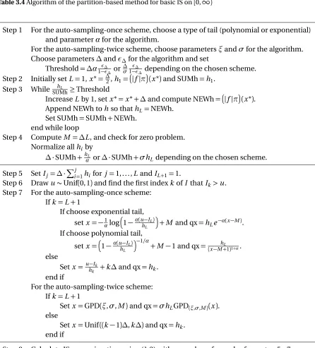
Table 3.4 Algorithm of the partition-based method for basic IS on[0,∞) . . . 44

Table 3.5 Parameters change between auto-sampling-once and auto-sampling-twice schemes . . . 45

Table 3.6 Computing time in seconds for Example 3.5 withN =10, 000 . . . 47

Table 3.7 Computing time in seconds of the partition-based method withN =10, 000, n=100 and∆=0.5, 0.1, 0.01 for Example 3.6 . . . 51

Table 3.8 Computing time in seconds of the simple Monte Carlo method withN = 1, 000, 000 and the partition-based method with∆=0.001 andN=10, 000 for Example 3.6 . . . 52

Table 3.9 Algorithm of the partition-based method for basic IS in the multidimensional spaces[0,∞)d _{. . . 64}

Table 4.1 Computing time in seconds of the likelihood ratio method withN =1, 000, 000 and the partition-based method with∆=1.5,ε_∆=0.01,ξ=100,σ=100 and N=10, 000 corresponding to Fig. 4.2 . . . 70

Table 4.2 Computing time in seconds of the likelihood ratio method withN =500, 000 and the partition-based method with∆=1.5,ε_∆=0.01,ξ=100,σ=100 and N=10, 000 corresponding to Fig. 4.4 . . . 72

(10)

Figure 1.1 All PDFs in Example 1.12 with the scaled target function. . . 13

Figure 1.2 Basic IS weight functions . . . 14

Figure 1.3 Histograms of samples fromπ,q1, . . . ,q6with the graph ofc r(x) . . . 15

Figure 1.4 One simulation of basic IS . . . 16

Figure 1.5 Jump analysis forq₃ . . . 17

Figure 1.6 The performance of simple Monte Carlo method . . . 18

Figure 1.7 Basic importance sampling performance . . . 19

Figure 1.8 Self-normalized importance sampling performance . . . 20

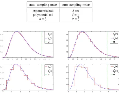
Figure 3.1 Proposal densities for parametersM =4, 10 andL=10, 25, 80 for Example 3.4 37 Figure 3.2 Histograms of the corresponding densities from Fig. 3.1 . . . 38

Figure 3.3 Basic IS performance of the corresponding densities from Fig. 3.1 . . . 39

Figure 3.4 Rescaled basic IS performance ofq₅andq₆from Example 1.12 . . . 40

Figure 3.5 Proposal densities with∆=0.1, 0.2, 0.4, 0.8 for Example 3.5 . . . 45

Figure 3.6 Performance of the corresponding densities from Fig. 3.5 with the auto-sampling-once scheme. . . 46

Figure 3.7 Performance of the corresponding densities from Fig. 3.5 with the auto-sampling-twice scheme. . . 46

Figure 3.8 Performance of the simple Monte Carlo method for Example 3.5 withN = 10, 000. . . 47

Figure 3.9 Performance of the simple Monte Carlo method for Example 3.5 withN = 1, 000, 000. . . 47

Figure 3.10 Target density and proposal densities with∆=0.5, 0.1, 0.01 for Example 3.6 . . 49

Figure 3.11 Performance of simple Monte Carlo method and basic IS with the correspond-ing densities from Fig. 3.10 . . . 51

Figure 3.12 Performance of the simple Monte Carlo method withN=1, 000, 000 and the partition-based method with∆=0.001 andN=10, 000 for Example 3.6. . . 52

Figure 3.13 Proposal densities with various parameters for Example 3.7 . . . 54

Figure 3.14 Self-normalized IS performance of the corresponding densities in Fig. 3.13 . . 55

Figure 3.15 Self-normalized IS performance with(M,L) = (6, 1). . . 56

Figure 3.16 The performance of a 4-dimensional partition-based proposal density in Example 3.8 . . . 63

Figure 4.1 Estimating delta of European call option . . . 69

Figure 4.2 Comparison between the likelihood ratio method and the partition-based method for estimating delta of European call option . . . 69

Figure 4.3 Estimating vega of European call option . . . 71

Figure 4.4 Comparison between the likelihood ratio method and the partition-based method for estimating vega of European call option . . . 72

Figure 4.5 Estimating theta of European call option . . . 73

(11)

Figure 4.9 Estimating gamma of European call option . . . 78 Figure 4.10 Comparison between the likelihood ratio method and the partition-based

method for estimating gamma of European call option . . . 79 Figure 4.11 Estimating delta, vega, theta, rho and gamma of European call option

simul-taneously by partition-based method . . . 82 Figure 4.12 Partition-based proposal densities in Example 4.7 and their corresponding

(12)

1 INTRODUCTION

Importance Sampling (IS) is a Monte Carlo-based simulation technique to estimate an expectation with respect to a distribution of interest using random samples drawn from another distribution. Normally, this technique is used when we have problems arising from our distribution of interest, which will be called thetarget distribution, and wish that we could use another distribution, which will be called aproposal distributionorimportance distribution, instead. We would like to use an ideal proposal distribution to generate samples to use in the estimation.

This technique is first used in rare event applications[17, 18, 14, 32, 2]where we want to estimate the expectation of a function that concentrates on the extremely-unlikely-to-be-visited region of the target distribution. In ordinary Monte Carlo method, we need to generate a huge number of samples directly from the target distribution to get just a sample falling inside that region. In many rare event applications, even when we set a pretty big number of samples, we could fail to have even one sample in that important region. Using IS, we can manage to estimate the expectation by sampling from another proposal distribution that has high probability around that important region of interest, hence the nameimportance sampling.

(13)

distribution together with associated weights that can be used as an empirical estimate of that target distribution. We can also use this empirical estimate to approximate the expectation of any given function with respect to the target distribution.

Apart from rare event applications and Bayesian inference which are two primary applications of IS, there are more uses IS can offer. In some applications where we have more than one target distribution, we can sample a single set of samples that can be used for all target distributions[1, 35]. This greatly reduces the amount of work from the direct simulation where we have to sample a separate set of samples for each target distribution. IS can also be a tool for estimating derivatives of expectations with respect to parameters of the underlying distribution[26, 27, 13, 3, 8]. This usage allows IS to attack some problems to which simple Monte Carlo method can hardly be directly applied. Moreover, IS is a key ingredient to develop Sequential Monte Carlo simulation in which IS is performed sequentially in time with samples and associated weights from the past time steps [9, 31, 7, 10, 5].

IS is considered as a variance reduction method to the ordinary Monte Carlo method. This depends on how well we choose a proposal distribution for sampling. If we pick a bad proposal distribution, it could blow the variance and has worse performance compared to a plain Monte Carlo method. A good proposal distribution actually depends on the target distribution and the function of interest.

To see the derivation of IS, we need to talk about a classical Monte Carlo method first. LetX be a random variable with a probability distributionπ, and f aπ−integrable function. Define the true expectation

µ = E[f(X)] = Eπ(f).

Since we assume that f is aπ−integrable function,µis finite. This is a convention to apply the Monte Carlo method. Also, because we are not interested in the obvious case, we assume thatf is not a constant function. A classical Monte Carlo estimator forµis

ˆ µπ = _N1

N

X

i=1

f(Xi), Xi

iid

∼π (1.1)

whereX_iiid∼πdenote thatX_i’s are independent and identically distributed with the distribution π. Also, we will denote byX ∼πwhenX has distributionπ. Please keep in mind that there areN number of samples in the formula of ˆµ_π, but we will suppressN for a short notation and focus on the distribution from which the samples are drawn.

(14)

used in this work. Most of the related work in the literature talk about just one kind of IS relying on their application, and most of foundation theory are available for only basic IS.

Throughout this work, we will express everything in the case of continuous space. For a discrete space, it can be derived in a similar manner and will be much easier to implement. To be able to apply IS, we assume that every probability distribution in this study is absolutely continuous with respect to the Lebesgue measure and has a density function. We will use the same notation for both probability measure and its probability density. When we write the integral without specifying the domain, we mean that the integral is taken on the whole domain which is allowed to be multidimensional.

1.1 Basic Importance Sampling

Consider a given pair of a target function and a target density(f,π). For a valid densityq, we can have that

Eπ(f) = Z

f(x)π(x)d x

=

Z

f(x)π(x)

q(x) q(x)d x

=Eq

_fπ

q

.

Define the weight function

w(·) =π(·)

q(·). (1.2)

Then, the basic IS estimator forµis

ˆ µq = 1

N N

X

i=1

w(Xi)f(Xi), Xi

iid

∼q. (1.3)

Now, let’s discuss more on the validity ofq. One may set an assumption onq to beπq(πis absolutely continuous with respect toq), and most current research use thatq(x) =0 =⇒ π(x) =0 as the assumption for a proposal density functionq, which is slightly stronger thanπq. However, we can relaxπqto a weaker assumption. Sinceµis finite, we can considerφ(d x) =f(x)π(x)d x as a finite measure. So, we can set an assumption for a legitimateqin the derivation step asφq. We will denote this by

(15)

and this is a weaker assumption thanπq.

Note that the weight function compensates the fact that we change the dominating measure fromπtoq.Xi’s in (1.1) are drawn according toπ, whileXi’s in (1.3) are drawn according toq. The regular Monte Carlo method has equal weight _N1 to all samples, but the basic IS method has weight

1

Nw(Xi)for sampleXi. The sample that properly represents the importance region will have high weight and become an important sample.

Remark 1.1. If we choose a proposal distributionqto beπitself, then it is equivalent to performing the classical Monte Carlo method.

1.2 Self-normalized Importance Sampling

In some situations especially in Bayesian inference applications where the normalizing constant for a posterior distribution is very hard to calculate, we can only deal with an unnormalized version of π. Consider a given pair of a target function and an unnormalized target density(f,p)where

π(x) =p(x) Z

andp(x)is known pointwise but the normalizing constantZ =Rp(x)d x is not known. For a valid density functionq, we can have that

Eπ(f) = Z

f(x)π(x)d x

= 1

Z

f(x)p(x)

q(x) q(x)d x

= 1

ZEq

_{f p}

q

≈ 1

Z

1 N

N

X

i=1

˜

w(X_i)f(X_i)

(X_iiid∼q)

where

˜

w(·) =p(·) q(·).

(16)

pq.

Then,

Z=

Z

p(x)d x

=

Z

p(x)

q(x)q(x)d x

≈ 1

N N

X

i=1

˜

w(X_i). (X_iiid∼q)

Thus, the self-normalized IS estimator forµis

˜ µq=

PN

i=1w˜(Xi)f(Xi)

PN

j=1w˜(Xj)

, Xi

iid

∼q. (1.4)

Remark 1.2. We can define the self-normalized weight function to be ˜w(·) =cp_q₍(·_·)₎for any constant multiplierc. All of these weight functions can induce the same self-normalized IS estimator ˜µq due to the cancellation in the ratio w˜(Xi)

PN j=1w˜(Xj)

.

Observe that the self-normalized weights are w˜(Xi)

PN j=1w˜(Xj)

summing up to one. Recall that for the

basic IS, the weights are _N1w(Xi)and may not be summed up to one. The self-normalized IS can be used to simulate the distribution of interestπby getting some samples{Xi}Ni=1from a proposal

distributionq with associated weights

(

Wi= ˜ w(X_i)

PN

j=1w˜(Xj)

)N

i=1

and approximating the distributionπby the empirical distribution

N

X

i=1

˜ w(Xi)

PN

j=1w˜(Xj)

δXi(d x)

(17)

especially in Bayesian inference, the proposal distributionqis selected as close as possible to the target distributionπwithout much consideration to the target functionf. However, the samples with associated weights can represent the distributionπ, and the corresponding empirical distribution can be used to approximate

Eπ(f)≈ Z

f(x) N

X

i=1

˜ w(Xi)

PN

j=1w˜(Xj)

δXi(d x) (Xi

iid ∼q)

=

N

X

i=1

˜ w(Xi)

PN

j=1w˜(Xj)

f(Xi)

which is (1.4).

1.3 Mathematical Theory

The derivation of IS is pretty simple, but this simulation technique has a huge benefit in many areas of applications described before. For whatever reasons or applications, we prefer to have the lowest possible variance for our IS. This section will provide mathematical statements about the convergence theorem in the form of Central Limit Theorem for each estimator: Monte Carlo, basic IS, and self-normalized IS. This obviously includes results on the expectation and the variance of each estimator. Moreover, the optimal proposal density for each kind of IS is identified here. Current work in this research area state these results without proper assumptions and precise details. In particular, the mathematical statements with proper assumptions and proofs of Theorem 1.5 and Theorem 1.10 have never been rigorously established in the past. The essential proofs, which are for Theorem 1.5, 1.7 and 1.10, will be provided in Chapter 2, and only the mathematical statements and some straightforward proofs are given in this Chapter.

1.3.1 Convergence Theorems

Let’s consider the Monte Carlo estimator ˆµ_πand the basic IS estimator ˆµq defined by (1.1) and (1.3), respectively. We can easily acquire the following theorem.

Theorem 1.3. E(µˆ_π) =µandE(µqˆ ) =µ. Also,

Var(µˆ_π) = 1 N

Z

(f(x)−µ)2π(x)d x

= 1

N

Z

f(x)2π(x)d x−µ2

(18)

and

Var(µqˆ ) = 1 N

Z

(f(x)π(x)−µq(x))2

q(x) d x

= 1

N

Z

f(x)2_π₍_x₎2

q(x) d x−µ

2

.

SinceE(µˆ_π) =E(µqˆ ) =µ, both ˆµ_πand ˆµq are unbiased estimators. Also, by the Central Limit Theorem, we have the following corollary.

Corollary 1.4. IfR f(x)2_π₍_x₎_{d x}_<_∞_,

p

N µˆ_π−µ−−−→D

N→∞ N

0,

Z

f(x)2π(x)d x−µ2

.

IfR f(x_q)2₍π_x(₎x)2 d x<∞,

p

N µqˆ −µ−−−→D

N→∞ N

0,

Z

f(x)2_π₍_x₎2

q(x) d x−µ

2

.

Now, consider the self-normalized IS estimator ˜µq defined by (1.4). Because of the ratio formula of ˜µq,E(µq˜ )and Var(µq˜ )cannot be directly derived. Generally,E(µq˜ )6=µ, so the self-normalized IS estimator is biased. However, by the Strong Law of Large Number together with the continuous mapping theorem, ˜µq converges toµalmost surely asN→ ∞. In the same way as the basic IS, we can also have a convergence theorem for self-normalized IS. The following theorem tells us about the asymptotic variance of the estimator in the form of Central Limit Theorem.

Theorem 1.5. IfR f(x_q)2₍π_x(₎x)2 d x andR π_q(₍x_x)₎2 d x are finite, then

p

N µq˜ −µ−−−→D

N→∞ N

0,

Z

(f(x)−µ)2_π₍_x₎2

q(x) d x

.

AVar(µq˜ ) =_N1 R (f(x)−_qµ₍_x)2₎π(x)2 d x will be called the asymptotic variance of the self-normalized IS estimator ˜µq. From Corollary 1.4 and Theorem 1.5, the rate of convergence for Monte Carlo, basic IS, and self-normalized IS isOp1

N

(19)

Corollary 1.6. If ( _q)₍_x₎( ) d x and _q(₍_x)₎ d x are finite, then

p

N µq˜ −µ−−−→D

N→∞ N

0,

Z

(f(x)−µ)2p(x)2 Z2_q(_x) d x

.

1.3.2 Optimal Proposal Densities

Unlike the classical Monte Carlo estimator which has a fixed variance, the variance of the basic IS estimator and the asymptotic variance of the self-normalized IS estimator can vary and can depend on the proposal distribution. If we can choose a good proposal densityq that makes Var(µqˆ )or AVar(µq˜ )lower than Var(µˆ_π), this will increase the precision of the IS estimate over the simple Monte Carlo method. However, a wrong choice of proposal distribution can make the estimation worse than that of the simple Monte Carlo method. We wish to find a proposal density that minimizes the variance of the basic IS estimator, and another for the asymptotic variance of the self-normalized IS estimator.

Theorem 1.7. The basic IS proposal density q that satisfies the validity condition fπq and minimizesVar(µqˆ )is

q_b∗(x) =R |f(x)|π(x)

|f(x)|π(x)d x. (1.5)

Remark 1.8. q_b∗always satisfies the validity for being a basic IS proposal density fπq_b∗

as well as the necessary condition for the convergence theorem for the basic IS estimators

Z

f(x)2π(x)2

q_b∗(x) d x<∞. Remark 1.9. If f is non-negative, then Var(µqˆ ∗

b) =0. This fact can be easily verified by calculating Var(µqˆ ∗

b)withq

∗

b(x) = f(x)π(x)

µ . Similarly, iff is non-positive, then Var(µqˆ ∗ b) =0.

Theorem 1.10. The self-normalized IS proposal density q that minimizes AVar(µq˜ )is

q_{s n}∗ (x) =R |f(x)−µ|p(x)

|f(x)−µ|p(x)d x (1.6)

(20)

Remark 1.11. q_{s n}∗ may not satisfy the self-normalized IS validity conditionpq_{s n}∗ nor the assump-tion of the convergence theorem for self-normalized IS estimatorsR f(x_q)∗2π(x)2

s n(x) d x,

R π(_x)2

qs n∗ (x)d x<∞. However, the validity conditionpq_{s n}∗ is satisfied for all target functionsf that is not constant at µon a set of finite measure. Hence,q_{s n}∗ satisfies the self-normalized IS validity conditionpq_{s n}∗ in most of real-life problems.

q_b∗ in Theorem 1.7 andq∗

s n in Theorem 1.10 will be called the optimal proposal densities for basic IS and self-normalized IS, respectively. Although we know what is the optimal proposal density for basic IS from Theorem 1.7, we cannot use it in reality because we do not knowR|f(x)|π(x)d x. Even in an easy case whenf is always non-negative, this term equals toµwhich is what we want to estimate at first, so we do not knowR|f(x)|π(x)d x in advance for the problem that we want to apply the basic IS method. The same argument also apply to the self-normalized IS method. We do not know in advance bothµand the normalizing constantR|f(x)−µ|p(x)d xneeded for the optimal proposal density for self-normalized IS acquired from Theorem 1.10.

1.4 Current Approaches

As discussed in the previous section, we cannot use the theoretically optimal proposal density in IS method. So, what do people do?

This research area of IS are growing fast in Statistics. What statisticians currently do for basic IS is to select a class of known distributions and try to find a distribution within that class which minimizes Var(µqˆ ). One of the best and recent methods is discussed in Subsection 1.4.1. To select a class of distributions for the proposal distributionq, statisticians focus on balancing weights of the samples,w(Xi)’s whereXi

iid

∼q, and try to minimize variance of these associated weights because dramatic fluctuation in weights usually results in a bad estimation. Hence, they want Varq(w)to be bounded. Consequently,

Z

π(x)2

q(x) d x<∞ (1.7)

is used as a rule of thumb[23, 34]in selecting a class of distributions forq. This is also the case in the self-normalized IS, since the weight function is the scalar multiplication version of that of basic IS. The equivalent rule of thumb for self-normalized IS is

Z

p(x)2

q(x) d x<∞,

(21)

1.4.1 Efficient Importance Sampling

There is a widely cited method calledefficient IS[28, 29]which may be praised as the best method for IS currently. It is an iterative method for basic IS that still has some limitations. It works only for a positive target function, and the proposal distribution has to be chosen in an exponential family of distributions. By the way, the rule of thumb (1.7) is broadly used to select such exponential family of distributions.

Suppose a class of known distributions indexed by a vector of auxiliary parameters

Q={qa|a∈A}

is carefully selected, whereAis a space of auxiliary parameters. Known distributions are used because they provide a quick access in sampling by various available software. The expression of Var(µqˆ _a)from Theorem 1.3 can be re-expressed as

σ2₍_a_{) =}_Var₍_µq_ˆ

a) =

Z

hg_a2(x)f(x)π(x)d x

where

ga(x) =log

_f(_x)π(_x)

µqa(x)

and

h(x) =epx+e−px−2.

Note thath is monotone, convex onR+, andh(x)≥x. Minimizingσ2(a)with respect toacalls for

nonlinear optimization. Consider the simpler function

v(a) =

Z

g_a2(x)f(x)π(x)d x

=

Z

log[f(x)π(x)]−log(µ)−log[qa(x)]

2

f(x)π(x)d x.

Leta∗and ˆabe the optimal parameters minimizingσ2₍_a₎_and_v₍_a₎_{, respectively. Then, we can have}

that

σ2₍_a_ˆ₎_≥_σ2₍_a∗₎_≥_h_[_v₍_a∗_)]_≥_h_[_v₍_a_ˆ_)]

which gives an upper bound and a lower bound forσ2(a∗), the smallest variance over the selected classQ.

(22)

and draws a number of samples from this distribution:x_i0iid∼qa0for alli=1, . . . ,R. Then, minimizing

ˆ

v_R(a) = 1 R

R

X

i=1

logf(x_i0)π(x_i0)−c−logq_a(x_i0) 2f(x_i0) π(x

0

i) qa0(x

0

i)

with respect toa andc, an intercept in place of the unknown log(µ), takes the form of a simple weighted linear least square problem, sinceQis chosen to be an exponential family of distributions. Starting froma₀,a₁is obtained as a result of solving the above generalized least square problem. The method can be iterated by using as initial sampler in any given round the optimized sampler from the previous round. The process continues until a stable solution forais reached, and that finalais used as ˆa. It is said that by experience, no more than 3 to 4 iterations are required to produce the final ˆa. Eventually,qaˆ is used as a proposal distribution for basic IS.

There is also an extension of efficient IS using a mixture of distributions for a proposal distribu-tion[20]. The use of a mixture of distributions can improve the performance of IS method in the case of heavy tailed or multi-modal target densities. Still, choosing a class of distributions at the beginning of the process is a serious issue. If an improper class of distributions is selected, the final result can be quite bad.

1.4.2 Truncated Importance Sampling

There is another readily applicable and theoretically justifiable approach for basic IS calledtruncated IS[16]. Since unfavorable IS estimation results usually come from harsh fluctuation in samples’

weights, this method suggests to truncate extreme weights by some constant depending onN, the number of samples. The truncated IS estimator forµis

ˆ µ0

q= 1 N

N

X

i=1

w0(Xi)f(Xi), Xi

iid

∼q. (1.8)

where

w0(Xi) =w(Xi)∧τN, the minimum ofw(Xi)andτN.

This estimator is biased, but the bias goes to zero asN → ∞, provided that lim

N→∞τN =∞.

Also, the variance of the estimator goes to zero asN → ∞, if Var_π(f)<∞and lim N→∞

τN

N =0. The recommended truncation rate in the literature isτN=pN. Although this method can reduce the sensitivity of importance sampling on the choice of the proposal distribution, it can slightly reduce the rate of convergence for the IS method and it is a biased method for basic IS.

(23)

overlook something that can cause extreme fluctuation of each term in the summation formula of the IS estimator. For example, consider basic IS withf(x) = e

x

2 4 p

x,π(x) =2e

−2x_{, and}_q₍_x_{) =} 5 2e−

5 2x.

Note that thisqsatisfies the rule of thumb (1.7). The basic IS weight function isw(x) =4₅ex2. So,

if we truncate the weight function with some threshold, we will truncate weights only for very large samples. But, each term in the summation formula of the truncated IS estimator from (1.8), w0(x)f(x) = 4₅pe4x_x ∧ τN

ex2 4 p

x, can blow up for both too large and too small samples which can cause high variance in estimation. Thus, the truncation cannot detect the problem with very small samples, and the estimation can be poor. Furthermore, consider another example withf(x) =x3_,

π(x) =2e−2x, andq(x) =4x e−2x which satisfies the rule of thumb (1.7). This setup yieldsw(x) =₂1_x andw0₍_X

i)f(Xi) =x

2

2 ∧ τNx3. The truncation will occur only for small samples, even though the

real problem is from large samples. This method may fail because it too focuses on the fluctuation of samples’ weights without taking into account the target functionf. For truncated IS, we should truncatew(x)f(x)instead ofw(x).

1.5 Examples

To understand better what is going on when IS is performed, the following example for IS is provided. This example also shows the insufficiency of the widely used rule of thumb (1.7) in choosing a proposal density.

Example 1.12. Let the target distributionπbe an exponential distribution with parameter mean1₂, and a target function

f(x) =x3.

The distributionπhas density

π(x) =2e−2x.

Consider applying IS method with the following proposal distributions:

1. a gamma distribution with shape parameter 4 and scale parameter 1₂

2. a no-name probability distribution whose density is directly proportional to a function

x3−3₄

e−2x

3. a Weibull distribution with scale parameter 1₂and shape parameter 2

(24)

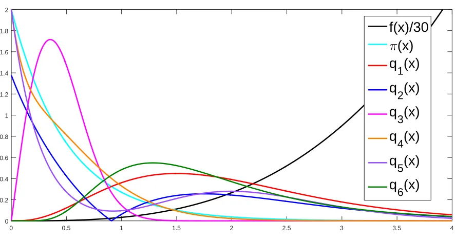
0 0.5 1 1.5 2 2.5 3 3.5 4 0

0.2 0.4 0.6 0.8 1 1.2 1.4 1.6 1.8 2

f(x)/30

π

(x)

q

1

(x)

q

₂

(x)

q

₃

(x)

q

4

(x)

q

5

(x)

q

6

(x)

Figure 1.1All PDFs in Example 1.12 with the scaled target function.

5. an equal mixture distribution between a gamma distribution with shape parameter 9 and scale parameter1₄and an exponential distribution with parameter mean1₄

6. a log-normal distribution with parameterµ=1₂andσ2=1₄

which have respectively the following densities:

q1(x) =8₃x3e−2x Gamma(4, 2) q2(x) =_Z1

2 x3−3₄

e−2x whereZ₂=3₂

1 2+

3 4

1₃

+ 3

4

2₃

e−2(34) 1 3

q3(x) =8x e−4x2 Weibull 1₂, 2

q4(x) =2(8x2+1)e−4x 1₂Gamma(3, 4) + 1₂Exp(4) q5(x) = 1024₃₁₅ x8+2e−4x 1₂Gamma(9, 4) + 1₂Exp(4) q6(x) =

p 2 p

πxe

−2(logx−12)2 _LogNormal 1 2,

1 4

.

(25)

0 1 2 3 4 5 0

2 4

w 6(x) 6 q₆(x)

0 1 2 3 4 5

0 2 4

w 1(x) 6 q

1(x)

0 1 2 3 4 5

0 2 4

w 2(x) 2 q₂(x)

0 0.5 1 1.5

0 2 4

w 3(x) 2 q

3(x)

0 1 2 3 4 5

0 2 4

w₄(x)

2 q 4(x)

0 1 2 3 4 5

0 2 4

w 5(x) 2 q

5(x)

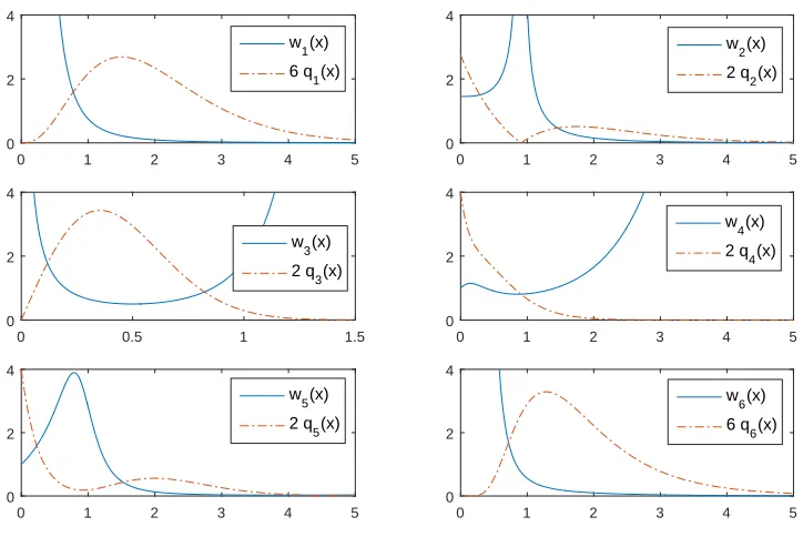
Figure 1.2Basic IS weight functions

example,q1is the optimal basic IS proposal density acquired from (1.5) in Theorm 1.7,q2is the

optimal self-normalized IS proposal density acquired from (1.6) in Theorm 1.10, and the true expectation isµ=R₀∞f(x)π(x)d x =3₄.

Basic IS method is considered first. All basic IS weight functions using Eq. 1.2 are presented in Fig. 1.2. We perform a simple Monte Carlo simulation and the basic IS with the proposalsq₁, . . . ,q₆, and compare the results with the theoretical expected value.

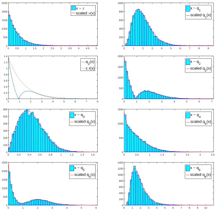
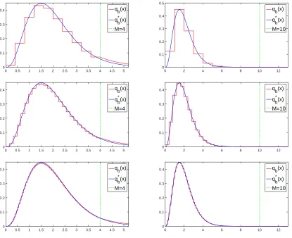
In this simulation, we sample 10,000 samples from each distribution:π,q1, . . . ,q6. Fig. 1.3 shows

histograms of these random samples. They tend to fit the corresponding densities very well. Since q2is a no-name distribution, we do not have a direct command in computer programming for

sampling from this distribution. To sample fromq2, we use the acceptance-rejection method from

Appendix A. Here, we use the exponential distribution with parameter mean 1.3, where its density is r(x) =_1.31 e−1.31 x, as a instrumental distribution toq₂in the acceptance-rejection method with the

bounding constantc =1.3×34× 1

Z2. We can easily verify that

q2(x)

c r(x)≤1 for allx≥0. The graph ofq2(x)

(26)

0 0.5 1 1.5 2 2.5 3 3.5 4 4.5 5 0 500 1000 1500 2000 2500

x ~ π

scaled π(x)

0 1 2 3 4 5 6 7 8 9 0 200 400 600 800 1000

x ~ q

1

scaled q

1(x)

0 1 2 3 4 5 6 7 8 0 0.2 0.4 0.6 0.8 1 1.2 1.4 q 2(x) c r(x)

0 1 2 3 4 5 6 7 0

500 1000 1500 2000

x ~ q₂

scaled q₂(x)

0 0.2 0.4 0.6 0.8 1 1.2 1.4 1.6 0 100 200 300 400 500 600

x ~ q

3

scaled q

3(x)

0 0.5 1 1.5 2 2.5 3 3.5 0

500 1000 1500

x ~ q₄

scaled q₄(x)

0 1 2 3 4 5 6

0 500 1000 1500 2000 2500

x ~ q

5

scaled q

5(x)

0 1 2 3 4 5 6 7 8 9 10 0 200 400 600 800 1000 1200 1400

x ~ q

6

scaled q

6(x)

Figure 1.3Histograms of samples fromπ,q1, . . . ,q6with the graph ofc r(x)

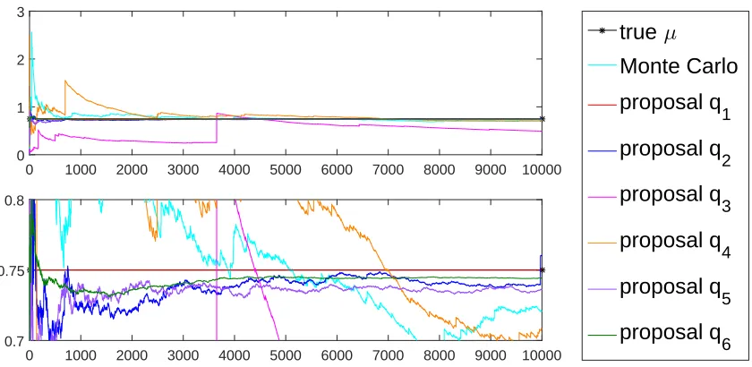
used, and then simply draw a sample according to that selected distribution in the mixture. Fig. 1.4 shows basic IS performance of each proposal distribution. Each sub-graph has a dif-ference scale for easier comparison. We sample 10,000 samples and approximateµusing (1.3). The x-axis is the number of samples,N, and the y-axis is the approximated expectation using the firstN samples. We can see that the proposalq1has the best performance, andq3has the worst

(27)

0 1000 2000 3000 4000 5000 6000 7000 8000 9000 10000 0

1 2 3

0 1000 2000 3000 4000 5000 6000 7000 8000 9000 10000 0.7

0.75 0.8

true

µ

Monte Carlo

proposal q

1

proposal q

2

proposal q

3

proposal q

4

proposal q

5

proposal q

6

Figure 1.4One simulation of basic IS

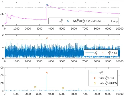
distribution, we perform many replications of this scenario. However, before we go into that simula-tion, the jump behavior of the proposal distributionsq3andq4is interesting. Later, we will see more

about this jump behavior, so we discuss this issue here using this example of the proposalq₃. From Fig. 1.2, we can see that the weight function for the proposalq3will blow up whenx is too

small or too large and this area has low probability to be sampled from. From the basic IS formula (1.3), we need the product of the weight function and the target function in the summation. In this case it is_qπ(x)

3(x)f(x) =

x2_e4x2−2x

4 and this amount will blow up for only largex. So, if we have a large

sample which rarely happen here, that term will increase the total summation drastically and result in a jump-up behavior. However, this large sample will have less effect on the total summation if we use a large total number of samples,N. A very low sample does not make the factor x2e4x

2₋₂_x 4

high in the calculation, although the corresponding weight is pretty high. Note that in this case, a sample which is greater than 1.6 may be considered a large sample. From Fig. 1.3, we can see that it is very hard to get a sample with really high value by sampling from the proposalq3. We will get

small samples most of the time so that each term of x2e4x

2₋₂_x

4 in the summation will keep low, and

when a big sample occurs, we get a jump. After a jump occurs, it will come back to keep getting lower and lower again until the next high sample appears and brings another jump. All information of this discussion is provided in Fig. 1.5.

(28)

0 1000 2000 3000 4000 5000 6000 7000 8000 9000 10000 0

0.5 1

µ₃(i) w(x₃(i))f(x₃(i)) > w(1.6)f(1.6) true µ

0 1000 2000 3000 4000 5000 6000 7000 8000 9000 10000 0

1 2

x

3 (i)

x

3 (i)

> 1.6

0 1000 2000 3000 4000 5000 6000 7000 8000 9000 10000 0

200 400 600

w

3 (i)

with x₃(i) > 1.6

with x₃(i) < 0.005

Figure 1.5Jump analysis forq3

results in the same graph for each proposal distribution to envisage variance of each estimator. The theoretical variance of the simple Monte Carlo estimator is Var(µˆ_π) =_N1 R2x6_e−2x_{d x}₋ 3

4

2

= 1

N

45 4 −

9 16

= 171 16N =

10.6875

N . Note that the true variance is not known in real-world problems, but this example composing of easy functions need to know the true expectation and variance for comparison purpose. Fig. 1.6 shows the performance of Monte Carlo method together with the plot ofµ±pVar(µˆ_π) =3₄±3

p 19 4

1 p

N indicating the true rate of convergence which is of the orderO(

1 p

(29)

0 1000 2000 3000 4000 5000 6000 7000 8000 9000 10000 0

0.5 1 1.5

µ µ± SD

Figure 1.6The performance of simple Monte Carlo method

From Fig. 1.7, the proposalq1, which is the optimal basic IS proposal densityq_b∗from Theorm 1.7,

seems to give the ideal result which is zero variance. This coincides with the theory. From Theorem 1.3,

Var(µqˆ ) = 1 N

Z

f(x)2π(x)2

q(x) d x−µ

2

.

We can calculate that Var(µqˆ ₁) =_N1 R ₂3x3e−2x d x− 34

2

= 1

N

3 2 3 8−

9 16

=0 for allN, the number of samples. This is the ideal proposal density for the basic IS with this specificf andπ. How could it be possible to get a zero variance in a Monte Carlo approximation using random samples? This is because in calculation,f multiplied withπjust perfectly cancels outq1and leaves just a constant:

f(x)π(x)

q1(x) = 3

4for any sample drawn fromq1. This explains why we obtain the true expectation 34for all

N since the beginningN=1, and this really coincides with the theory about zero variance for the optimal proposal density in the case of non-negativef.

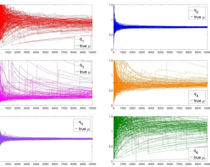
Now, a very interesting observation is that according to Fig. 1.4, Fig. 1.6 and Fig. 1.7, the proposal q6tends to have much smaller variance comparing to the simple Monte Carlo method. However,

we can check thatR f(x_q)2π(x)2

6(x) d x = ∞which means Var(µqˆ 6) =∞for allN. This seems like a

contradiction. Also, we can check that Var(µqˆ ₂) =Var(µqˆ ₃) =Var(µqˆ ₄) =∞. We can clearly notice the jump behavior in bothq3andq4cases, and there are a small number of jumps inq2,q5andq6cases.

Normally, if we have a jump behavior in basic IS with a proposal distribution, then that proposal distribution may yield an infinite variance of the corresponding basic IS estimator. We will continue to discuss this issue together with the conflict about the simulation performance ofq6versus its

theoretical aspect in Chapter 3.

Now, the self-normalized IS is performed using the same setup of f,p =π,q1, . . . ,q6. From

(30)

Figure 1.7Basic importance sampling performance

optimal densityq_{s n}∗ acquired from Theorem 1.10.

Fig. 1.8 shows the self-normalized IS result of all proposal distributions using the same sampled data when we perform the basic IS method. From Theorem 1.5, the asymptotic variance for the proposalqis given by

AVar(µq˜ ) = 1 N

Z

(f(x)−µ)2π(x)2 q(x) d x.

We can check that the asymptotic variance for the proposalsq1,q3,q4andq6are all infinite. Indeed,

(31)

Figure 1.8Self-normalized importance sampling performance

proposalq₂is₈9_N 14+7(613) +4(623)

e−2(613)

≈1.18603N . We can see thatq1,q3,q4andq6yield the jump

behavior indicating very poor performance due to infinite asymptotic variance. We can see that there are both jump-up and jump-down behaviors unlike the basic IS method. The jump behavior is interesting and we will explain more here using this example.

For the case of non-negative f, in basic IS method, the jump behavior usually occurs when weights in the summation of the estimator formula are very high, and only the jump-up behavior can occur. We should observe that from Fig. 1.2,q₁andq₆have similar graphs of densities and weight functions, butq1which is the optimal proposal density does not have the jump behavior

whileq6does. This is becausef also has an effect on the summation formula. From (1.4), if the new

(32)

functionf may make the adding term in numerator so huge that the whole numerator dominates the increase in denominator which has no effect from f, hence the jump-up behavior. We can see that not onlyπandq butf has an effect on the performance of IS method. The jump-up or jump-down behavior really depends on allp,q, andf, but neither behaviors are good. The jump behavior usually suggests that the estimator has infinite variance. However, there are some cases where the variance or asymptotic variance can be bounded as shown in the case of ourq5here. So,

we cannot judge by just checking the appearance of the jump behavior.

It is quite hard to choose a good proposal density for self-normalized IS. The optimal one is usually an unnatural density as we may realize even in this one-dimensional problem. In the same way as basic IS, we cannot use the optimal density in reality due to the unknownµin the first place.

An important thing to notice from this example is thatq4satisfies the rule of thumb (1.7) in

choos-ing a proposal density, but it obviously has a bad performance for both basic and self-normalized IS methods. Also, if the proposal distribution is not well chosen such asq₃andq₄, the IS method may be worse than the regular Monte Carlo method.

(33)

2 MATHEMATICAL PROOFS

The proofs for Theorem 1.5, 1.7 and 1.10 are separated from their statements in Section 1.3 and presented in this chapter.

2.1 Proof of Theorem 1.5

This section provides the proof of Theorem 1.5. The proof relies on the so-called delta method which is, provided by the aid of Taylor expansions, a generalization of Central Limit Theorem. In the proof, we will really see why we need some additional assumptions which requireR f(x_q)2₍π_x₎(x)2 d x andR π_q(₍x_x)₎2 d x to be finite. Note that there is a proof given in[11], but that proof does not cite the reference properly.

Proof of Theorem 1.5. We will apply the delta method from Appendix B to ˜µq. Let

Ai=w˜(Xi)f(Xi) and Bi=w˜(Xi) where Xi

i i d

∼ q so that the random vectors(Ai,Bi)are independent and identically distributed. Then,E(A1) =µZ andE(B1) =Z. Denote the variance ofA1, the variance ofB1, and the covariance

(34)

σ2

A=

Z

p(x) q(x)f(x)

2

q(x)d x−(µZ)2

=Z2

Z

π(x)2f(x)2

q(x) d x−µ

2 . Also, σ2 B= Z

p(x) q(x)

2

q(x)d x−Z2

=Z2

Z

π(x)2

q(x) d x−1

and

σAB=E w˜(X1)f(X1)−µZ(w˜(X1)−Z)

=Ew˜(X1)2f(X1)−Zw˜(X1)f(X1)−µZw˜(X1) +µZ2

=Z2

Z

π(x)2f(x) q(x) d x−

Z

π(x)f(x)d x−µ

Z

π(x)d x+µ

=Z2

Z

π(x)2f(x)

q(x) d x−µ

.

Note that by Holder’s inequality,

Z

π(x)2_f₍_x₎

q(x) d x =

Z

π(x)f(x)

p

q(x)

π(x)

p

q(x)

d x

≤

Z

π(x)2_f₍_x₎2

q(x) d x

1₂Z

π(x)2

q(x) d x

1₂

.

Thus, by the assumption thatR f(x_q)2₍π_x(₎x)2 d x andR π_q(₍x_x)2₎ d x are finite, allσ2

A,σ2B andσAB are finite. By Central Limit Theorem, we have that

p N 1 N N X

i=1

˜

w(Xi)f(Xi), 1 N

N

X

i=1

˜ w(Xi)

−(µZ,Z)

D

−−−→

N→∞ N2(0,Σ)

where

Σ=

σ2

A σAB σAB σ2

B

(35)

Now, letg(a,b) =_b. We have that g 1 N N X

i=1

˜

w(Xi)f(Xi), 1 N

N

X

i=1

˜ w(Xi)

=µq˜ .

We simply calculateg(µZ,Z) =µand∇T_~µ :=∇g(µZ,Z)T = (_Z1,−Zµ). Then,

∇T_~µ Σ∇~µ=_Z1₂σ2A+ µ2

Z2σ 2

B−2 µ Z2σAB =

Z

π(x)2_f₍_x₎2

q(x) d x−µ

2

+µ2

Z

π(x)2

q(x) d x−1

−2µ

Z

π(x)2_f₍_x₎

q(x) d x−µ

=

Z

π(x)2₍_f₍_x₎₋_µ₎2

q(x) d x.

Applying the delta method, we obtainpN µq˜ −µ−−−→D

N→∞ N

0,R (f(x)−_qµ₍_x)2₎π(x)2 d x.

2.2 Proof of Theorem 1.10

The proof of Theorem 1.10 is given in this section. Moreover, the proof of Theorem 1.7, which can be found in[19, 30, 25], is provided in details here. We will see the way to come up with the proof for Theorem 1.7 which is to seek for a nominee for the optimal proposal density and then show that such nominee really is the optimal one. Then, we can use this line of proof to prove Theorem 1.10. We now begin with the proof of Theorem 1.7.

Proof of Theorem 1.7. To minimizeR f(x_q)2₍π_x(₎x)2 d x subject to a constraintRq(x)d x =1, we apply the method of Lagrange multipliers for calculus of variations from Appendix C at least to find the candidate for the minimizer. Note that we also have constraintsπandqbeing non-negative. Let

L(x,q,λ) = f(x)

2_π₍_x₎2

q(x) +λq(x).

Setting

∂L ∂q =−

f(x)2π(x)2

q(x)2 +λ=0,

we have that

q(x) =

v

tf(x)2π(x)2

λ =

|f(x)|π(x)

p

λ .

SinceRq(x)d x=1, we have thatq(x) =R |f(x)|π(x)

(36)

we will show that this

q_b∗(x) =R |f(x)|π(x)

|f(x)|π(x)d x

yields the minimum variance among all valid basic IS proposal densities. Obviously,fπq_b∗. Letq be any density satisfyingfπq. Then,

Z

f(x)2π(x)2 q_b∗(x) d x=

Z

f(x)2π(x)2

|f(x)|π(x)

R

|f(x)|π(x)d x d x=

Z

|f(x)|π(x)d x

2

=

Z

|f(x)|π(x)

q(x) q(x)d x

2

=E

_|_f(_X)|π(_X)

q(X)

2

, X ∼q

≤E

|f(X)|π(X) q(X)

2

=

Z

f(x)2π(x)2

q(x)2 q(x)d x

=

Z

f(x)2π(x)2 q(x) d x

by Jensen’s inequality. Hence,

Var(µqˆ ∗ b) =

1 N

Z

(f(x)2π(x)2

q_b∗(x) d x−µ

2

≤ 1

N

Z

(f(x)2_π₍_x₎2

q(x) d x−µ

2

=Var(µqˆ )

which completes the proof.

Now, we will follow analogous line of proof for Theorem 1.10. Note that there is a statement with proof given in[11], but that statement does not talk about the validity of the proposal density.

Proof of Theorem 1.10. Let

L(x,q,λ) =π(x)

2₍_f₍_x₎₋_µ₎2

q(x) +λq(x).

Setting

∂L ∂q =−

(f(x)−µ)2_π₍_x₎2

q(x)2 +λ=0,

we have that

q(x) =

v

t(f(x)−µ)2π(x)2

λ =

|f(x)−µ|π(x)

p

(37)

Since q(x)d x =1, we have thatq(x) = R

|f(x)−µ|π(x)d x =R|f(x)−µ|p(x)d x. Now, we will show that this candidate

q_{s n}∗ (x) =R |f(x)−µ|p(x)

|f(x)−µ|p(x)d x

yields the minimum asymptotic variance. Letqbe any density function such thatpq.

Z

(f(x)−µ)2π(x)2 qs n∗ (x)

d x=

Z

(f(x)−µ)2π(x)2

|f(x)−µ|π(x)

R

|f(x)−µ|π(x)d x d x =

Z

|f(x)−µ|π(x)d x

2

=

Z

|f(x)−µ|π(x)

q(x) q(x)d x

2

=

E

_|_f(_X)₋µ_|π(_X)

q(X)

2

, X ∼q

≤E

_|_f₍_X₎₋_µ_|_π₍_X₎

q(X)

2

=

Z

(f(x)−µ)2_π₍_x₎2

q(x)2 q(x)d x

=

Z

(f(x)−µ)2_π₍_x₎2

q(x) d x

(38)

3 PARTITION-BASED METHOD

Before the partition-based method is presented, we continue the discussion of Example 1.12 here. Table 3.1 shows the related integrals for proposal distributions in Example 1.12. Surprisingly, the optimal densities for both basic (q1=qb∗) and self-normalized (q2=qs n∗ ) IS have integral

R π(x)2

qi(x) d x=

∞. This integral is the current rule of thumb (1.7) widely used by statisticians as a criterion to choose a good proposal density for both basic and self-normalized IS. More surprisingly,q2which is the

Table 3.1Related integrals for proposal distributions in Example 1.12

q_i R π_q(x)2 i(x)d x

R f(x)2_π₍_x₎2

qi(x) d x

R (f(x)−µ)2_π₍_x₎2

qi(x) d x

q1=q_b∗ ∞ 0.5625 ∞

q2=qs n∗ ∞ ∞ ≈1.18603

q3 ∞ ∞ ∞

q4 ≈1.11072 ∞ ∞

q₅ ≈1.93144 ≈1.34172 ≈1.50409

(39)

optimal density for self-normalized IS does not satisfy the convergence assumption of Theorem 1.5. This does not violate any theory. From Remark 1.11,q∗

s nis just the probability density function that minimizesR (f(x)−_qµ₍_x)2₎π(x)2 d xand may not satisfy the self-normalized IS validity condition nor the assumption of the convergence theorem for self-normalized IS estimators. Here,q2 attains

the minimum ofR (f(x)_q−µ)2π(x)2

2(x) d x at 9 8(14+7

3 p

6+4p336)e−2p36_≈_{1.18603. It satisfies}_p _q 2, but

R f(x)2_π₍_x₎2

q2(x) d x, R π(x)2

q2(x)d x =∞. Another interesting point is that R π(x)2

q4(x) d x = π

2p2 ≈1.11072<∞,

soq4satisfies the rule of thumb (1.7). However, it is a bad proposal density for both basic IS and

self-normalized IS as we can see from Fig. 1.7 and Fig. 1.8. Thus, the condition (1.7) is not a satisfying criterion for choosing a good proposal density for IS method. If we really pay attention to the convergence theorem of IS estimator, we can get closer to the answer. The criterion should rather be

Z

f(x)2π(x)2

q(x) d x<∞

for basic IS, and

Z

f(x)2_p₍_x₎2

q(x) d x,

Z

p(x)2

q(x)d x<∞

for self-normalized IS. A good example for this isq₅which hasR f(x_q)2p(x)2

5(x) d x=

37/4357/8 29 17₂ +6

p

2

1 8_π

≈

1.34172<∞andR p_q(x)2

5(x)d x=

31/4351/8 225/8 4+2

p

2

1 2_π

≈1.93144<∞. Therefore, we have a finite vari-ance, Var(µqˆ ₅) = _N1 R f(x_q)2p(x)2

5(x) d x−µ

2_≈ 1.34172−0.5625

N = 0.77922N and a finite asymptotic variance, AVar(µq˜ ₅) = _N1 R (f(x)−_qµ)2π(x)2

5(x) d x = 1

N

31/4351/8 21/8 4+2

p

2

1

2₊33/4357/8 12

17 2 +6

p

2

1 8

− 352

1₂₉π

27 ≈ 1.50409_N .

Both basic IS and self-normalized IS performances ofq5are really good.

Although we cannot always use the theoretically optimal proposal density in IS method in reality, we may be able to find a nice proposal density that gives a really pleasant outcome and at the same time satisfies all theoretical assumptions we need. To get an idea of how this work can come about, we consider the case of basic IS first. From Example 1.12, we can see from Fig. 1.7 that the proposal densityq6has a good performance, and from Fig. 1.1 that the probability density function ofq6is very

closed to the optimal proposal densityq1. This gives us an idea that a good proposal density should be

closed to the optimal one,q_b∗for basic IS andq∗

s nfor self-normalized IS. A question that should come to one’s mind is why the proposalq6brings about a nice result despite the fact that Var(µqˆ 6) =∞.

From Theorem 1.3, we have that Var(µqˆ ₆) = _N1

_R_∞

0 2

p

2πx7e2(logx−12) 2

−4x _{d x}₋₍3 4)2

and one can check that the part that make the variance infinite is the integral around the neighborhood of zero, sayR₀ε2p2πx7e2(logx−12)

2

−4x _{d x}₌_∞_,_{ε >}_{0. From the basic IS formula (1.3),each term in the} summation with the proposal densityq6is f(_qx₆)₍π_x(₎x)=

p

2πx4_e2(logx−12) 2

(40)

Table 3.2All assumptions for proposal distributions/densities

Basic IS Self-normalized IS

Given f,π f,p

Validity fπq pq

Convergence R f(x_q)2₍π_x(₎x)2d x<∞ R f(x_q)2₍p_x(₎x)2d x, R p_q(₍x_x)₎2d x < ∞

to infinity asx goes to 0. So, the jump behavior will arise when we get a sample too closed to 0. According to the probability density functionq6from Fig. 1.1, most of the time we will get random

samples not too close to 0. Thus, the jump problem rarely happens in the simulation, and that makesq₆look good enough to be used as a proposal density. However, we cannot deny the fact that it brings about infinite variance. Therefore, in this chapter, we propose a valid proposal density that gives a really pleasant outcome, guarantee finite variance (for basic IS or asymptotic variance for self-normalized IS) of the estimator, and satisfies the assumption for the associated convergence theorem.

3.1 Sufficient Conditions

The derivation of both kinds of IS from Section 1.1 and 1.2 needs the assumption for a legitimate proposal distribution. Also, Corollary 1.4 and Theorem 1.5 tell us all the assumptions for a proposal density to have the associated convergence theorem. Table 3.2 summarizes all of these assumptions. Note that the assumptionR f(x_q)2₍π_x₎(x)2d x <∞also implies the boundedness of Var(µqˆ ), and the assumptionR f(x_q)2₍p_x(₎x)2d x , R p_q(₍x_x)₎2d x < ∞also implies the boundedness of AVar(µq˜ ). Therefore, all we need for a good proposal distribution are