Modeling Word Forms Using Latent Underlying Morphs and Phonology

Modeling Word Forms Using Latent Underlying Morphs and Phonology

Department of Computer Science, Johns Hopkins University {ryan.cotterell,npeng1,eisner_}@jhu.edu

Abstract

The observed pronunciations or spellings of words are often explained as arising from the “underlying forms” of their mor-phemes. These forms are latent strings that linguists try to reconstruct by hand. We propose to reconstruct them automatically at scale, enabling generalization to new words. Given some surface word types of a concatenative language along with the abstract morpheme sequences that they ex-press, we show how to recover consistent underlying forms for these morphemes, together with the (stochastic) phonology that maps each concatenation of underly-ing forms to a surface form. Our technique involves loopy belief propagation in a nat-ural directed graphical model whose vari-ables are unknown strings and whose con-ditional distributions are encoded as finite-state machines with trainable weights. We define training and evaluation paradigms for the task of surface word prediction, and report results on subsets of 7 languages.

1 Introduction

How is plurality expressed in English? Compar-ing cats ([kæts]), dogs ([dOgz]), and quizzes ([kwIzIz]), the plural morpheme evidently has at least three pronunciations ([s], [z], [Iz]) and at

least two spellings (-s and-es). Also, consider-ing sconsider-ingularquiz, perhaps the “short exam” mor-pheme has multiple spellings (quizz-,quiz-).

Fortunately, languages are systematic. The re-alization of a morpheme may vary by context but is largely predictable from context, in a way that generalizes across morphemes. In fact, gener-ative linguists traditionally posit that each mor-pheme of a language has a singlerepresentation shared across all contexts (Jakobson, 1948; Ken-stowicz and Kisseberth, 1979, chapter 6). How-ever, this string is a latent variable that is never observed. Variation appears when thephonology

of the language maps theseunderlying represen-tations (URs)—in context—to surface represen-tations (SRs) that may be easier to pronounce. The phonology is usually described by a grammar that may consist of either rewrite rules (Chomsky and Halle, 1968) or ranked constraints (Prince and Smolensky, 2004).

We will review this framework in section 2. The upshot is that the observed words in a language are supposed to be explainable in terms of a smaller underlying lexicon of morphemes, plus a phonol-ogy. Our goal in this paper is to recover the lexicon and phonology (enabling generalization to new words). This is difficult even when we are told which morphemes are expressed by each word, be-cause the unknown underlying forms of the mor-phemes must cooperate properly with one another and with the unknown phonological rules to pro-duce the observed results. Because of these in-teractions, we must reconstruct everything jointly. We regard this as a problem of inference in a di-rected graphical model, as sketched in Figure 1.

This is a natural problem for computational lin-guistics. Phonology students are trained to puzzle out solutions for small datasets by hand. Children apparently solve it at the scale of an entire lan-guage. Phonologists would like to have grammars for many languages, not just to study each lan-guage but also to understand universal principles and differences among related languages. Auto-matic procedures would recover such grammars. They would also allow comprehensive evaluation and comparison of different phonological theories (i.e., what inductive biases are useful?), and would suggest models of human language learning.

Solving this problem is also practically impor-tant for NLP. What we recover is a model that can generate and help analyze novel word forms,1 which abound in morphologically complex lan-guages. Our approach is designed to model sur-facepronunciations(as needed for text-to-speech and ASR). It might also be applied in practice 1_{An analyzer would require a prior over possible analyses.}

Our present model defines just the corresponding likelihoods, i.e., the probability of the observed wordgiveneach analysis.

433

rizajgn z eɪʃ#n dæmn

rizajgn#eɪʃ#n rizajgn#z dæmn#z dæmn#eɪʃ#n

rˌɛ.zɪg.nˈeɪ.ʃ#n ri.zˈajnz dæmz dˌæm.nˈeɪ.ʃ#n

rˌɛzɪgnˈeɪʃn̩ rizˈajnz dˈæmz dˌæmnˈeɪʃn̩

1) Morpheme URs

2) Word URs

3) Word SRs

Concatenation (e.g.)

Phonology (PFST)

Phonetics

resignation resigns damns damnation

2 M

2 U

2 S

4) Word Observations

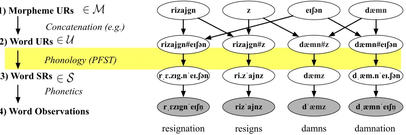
Figure 1: Our model as a Bayesian network, in which surface forms arise from applying phonology to a concatenation of underlying forms. Shaded nodes show the observed surface forms for four words:resignation,resigns,damns, anddamnation. The graphical model encodes their morphological relationships using latent forms. Each morpheme UR at layer 1 is generated by the lexicon modelMφ(a probabilistic finite-state automaton). These are concatenated into various word URs at layer 2. Each SR at layer 3 is generated using the phonology modelSθ(a probabilistic finite-state transducer). Layer 4 derives observable phonetic forms from layer 3. This deletes unpronounced symbols such as syllable boundaries, and translates the phonemes into an observed phonetic, articulatory, or acoustic representation. However, our present paper simply merges layers 3 and 4: our layer 3 does not currently make use of any unpronounced symbols (e.g., syllable boundaries) and we observe it directly.

to model surfacespellings(as needed for MT on text). Good morphological analysis has been used to improve NLP tasks such as machine translation, parsing, and NER (Fraser et al., 2012; Hohensee and Bender, 2012; Yeniterzi, 2011).

Using loopy belief propagation, this paper at-tacks larger-scale learning problems than prior work on this task (section 8). We also develop a new evaluation paradigm that examines how well an inferred grammar predictsheld-out SRs. Un-like previous algorithms, we do not pre-restrict the possible URs for each morpheme to a small or structured finite set, but use weighted finite-state machines to reason about the infinite space of all strings. Our graphical model captures the standard assumption that each morpheme has a single UR, unlike some probabilistic learners. However, we do not try to learn traditional ordered rules or con-straint rankings like previous methods. We just search directly for a probabilistic finite-state trans-ducer that captures likely UR-to-SR mappings. 2 Formal Framework

We urge the reader to begin by examining Fig-ure 1, which summarizes our modeling approach through an example. The upcoming sections then give a formal treatment with details and discus-sion. Section 2 describes the random variables in Figure 1’s Bayesian network, while section 3 describes its conditional probability distributions. Sections 4–5 give inference and learning methods. Amorphemeis a lexical entry that pairs form with content (Saussure, 1916). Its form is a

morph—a string of phonemes. Its content is a bundle of syntactic and/or semantic properties.2

Note that in this paper, we are nonstandardly us-ing “morph” to denote anunderlying form. We assume that all underlying and surface represen-tations can be encoded as strings, over respective alphabetsΣuandΣs. This would be possible even for autosegmental representations (Kornai, 1995). A language’s phonological system thus consists of the following components. We denote each im-portant set by a calligraphic letter. We use the cor-responding uppercase letter to denote a function to that set, the corresponding lowercase letter as a variable that ranges over the set’s elements, and a distinguished typeface for specific elements.

• Ais a set of abstract morphemes such as‚qu’i„z

andp†l’u„r$a†l. These are atoms, not strings.

• M = Σ∗_u is the space of possible morphs:

concrete UR strings such as /kwIz/ or /z/.

• M : _{A → M}is the lexicon that maps each morpheme a to an underlying morph m = M(a). We will findM(a)for eacha. • U = (Σu∪ {#})∗ is the space of underlying

representations for words, such as /kwIz#z/. • U : M∗ _{→ U combines morphs. A word}

is specified by a sequence of morphemes~a=

a1, a2, . . ., with concrete formsmi=M(ai).

That word’s underlying form is then u = U(m1, m2, . . .)∈ U.

2_{This paper does not deal with the content. However,}

• S = Σ∗_s is the space of surface

representa-tions for words, such as [kwIzIz].

• S : _{U → S} is the phonology. It maps an underlying formuto its surface forms. We will find this functionSalong withM. We assume in this paper that U simply con-catenates the sequence of morphs, separating them by the morph boundary symbol #: u =

U(m1, m2, . . .) = m1#m2#· · ·. However, see

section 4.3 for generalizations.

The overall system serves to map an (abstract) morpheme sequence~a _{∈ A}∗ to a surface word s _{∈ S}. Crucially, S acts on the underlying form

u of the entire word, not one morph at a time. Hence its effect on a morph may depend on con-text, as we saw for English pluralization. For ex-ample,S(/kwIz#s/) =[kwIzIz]—or if we were to

apply our model to orthography, S(/quiz#s/) =

[quizzes]. S produces a single well-formed

sur-face form, which is not arbitrarily segmented as [quiz-zes] or [quizz-es] or [quizze-s].

3 Probability Model

Our goal is to reconstruct the lexiconM and

mor-phophonologyS for a given language. We

there-fore define prior probability distributions over them. (We assumeΣ_u,Σ_s,_A, U are given.)

For each morpheme a _{∈ A}, we model the morphM(a)_{∈ M}as an IID sample from a proba-bility distributionMφ(m).3 This model describes what sort of underlying forms appear in the lan-guage’s lexicon.

The phonology is probabilistic in a similar way. For a word with underlying formu _{∈ U}, we

pre-sume that the surface formS(u)is a sample from

a conditional distributionSθ(s | u). This single sample appears in the lexical entry of the word typeand is reused for all tokens of that word.

The parameter vectorsφandθare specific to the

language being generated. Thus, under our gener-ative story, a language is created as follows:

1. Sampleφandθfrom priors (see section 3.4).

2. For eacha∈ A, sampleM(a)∼Mφ. 3. Whenever a new abstract word~a=a1, a2· · ·

must be pronounced for the first time, con-structuas described in section 2, and sample S(u)_∼Sθ(· |u). Reuse thisS(u)in future.

Note that we have not specified a probability distribution over abstract words~a, since in this

3_{See section 3.3 for a generalization toMφ(m|a).}

paper, these sequences will always be observed. Such a distribution might be influenced by the se-mantic and syntactic content of the morphemes. We would need it to recover the abstract words if they wereunobserved, e.g., when analyzing novel word forms or attempting unsupervised training.

3.1 Discussion: Why probability?

A language’s lexiconM and morphophonologyS

are deterministic, in that each morpheme has a sin-gle underlying form and each word has a sinsin-gle surface form. The point of the language-specific distributionsMφandSθis to aid recovery of these forms by capturingregularitiesinMandS.

In particular,Sθconstitutes a theory of the regu-lar phonology of the language. Its high-probability sound changes are the “regular” ones, while irreg-ularities and exceptions can be explained as occa-sional lower-probability choices. We prefer a the-orySθthat has high likelihood, i.e., it assigns high probability (≈1) to each observed formsgiven its

underlyingu. In linguistic terms, we prefer

pre-dictive theories that require few exceptions. In the linguistic community, the primary mo-tivation for probabilistic models of phonology (Pierrehumbert, 2003) has been to explain “soft” phenomena: synchronic variation (Sankoff, 1978; Boersma and Hayes, 2001) or graded acceptabil-ity judgments on novel surface forms (Hayes and Wilson, 2008). These applications are orthog-onal to our motivation, as we do not observe any variation or gradience in our present exper-iments. Fundamentally, we use probabilities to measure irregularity—which simply means unpre-dictability and is a matter of degree. Our objective function will quantitatively favor explanations that show greater regularity (Eisner, 2002b).

A probabilistic treatment also allows rela-tively simple learning methods (e.g., Boersma and Hayes (2001)) since inference never has to back-track from a contradiction. Our method searches a continuous space of phonologiesSθ, all of which are consistent with every mappingS. That is, we

es-w

ɛ

t

ɾ

w

ɛ

r

ə

Next Input Character Input Right Context

Input Left Context

Output Left Context

Output Right Context Stochastic Choice

Of Edit in Context C

Figure 2: Illustration of a contextual edit process as it pro-nounces the English wordwetterby transducing the under-lying /wEt#@r/ (after erasing #) to the surface [wER@r]. At the point shown, it is applying the “intervocalic alveolar flap-ping” rule, replacing /t/ in this context by applyingSUBST(R).

cape such low-likelihood solutions, much as back-tracking escapes zero-likelihood solutions.

3.2 Mapping URs to SRs: The phonologySθ We currently modelSθ(s | u) as the probability that a left-to-rightstochastic contextual edit pro-cess(Figure 2) would edituintos. This probabil-ity is a sum over all edit sequences that produces

fromu—that is, alls-to-ualignments.

Stochastic contextual edit processes were de-scribed by Cotterell et al. (2014). Such a pro-cess writes surface strings ∈ Σ∗_s while reading

the underlying stringu ∈ Σ∗_u. If the process has

so far consumed some prefix of the input and pro-duced some prefix of the output, it will next make a stochastic choice among2_|Σs|+ 1possible ed-its. Edits of the formSUBST(c)orINSERT(c)(for c_∈Σs) appendcto the output string. Edits of the formSUBST(c)orDELETEwill (also) consume the next input phoneme; if no input phonemes remain, the only possible edits areINSERT(c)orHALT.

The stochastic choice of edit,given context, is governed by a conditional log-linear distribution with feature weight vectorθ. The feature functions

may look at a bounded amount of left and right input context, as well as left output context. Our feature functions are described in section 6.

OurnormalizedprobabilitiesSθ(s | u)can be computed by a weighted finite-state transducer, a crucial computational property that we will ex-ploit in section 4.2. As Cotterell et al. (2014) explain, the price is that our model is left/right-asymmetric. The inability to condition directly on the right output context arises from local normal-ization, just like “label bias” in maximum entropy Markov models (McCallum et al., 2000). With

certain fancier approaches to modelingSθ, which we leave to future work, this effect could be miti-gated while preserving the transducer property.

3.3 Generating URs: The lexicon modelMφ In our present experiments, we use a very simple lexicon modelMφ, so that the burden falls on the phonologySθto account for any language-specific regularities in surface forms. This corresponds to the “Richness of the Base” principle advocated by some phonologists (Prince and Smolensky, 2004), and seems to yield good generalization for us. Specifically, we say all URs of the same length have the same probability, and the length is geo-metrically distributed with mean(1/φ)−1. This is

a 0-gram model with a single parameterφ∈(0,1],

namelyMφ(m) = ((1−φ)/|Σu|)|m|·φ.

It would be straightforward to experiment with other divisions of labor between the lexicon model and phonology model. A 1-gram model forMφ would also model which underlying phonemes are common in the lexicon. A 2-gram model would model the “underlying phonotactics” of morphs, though phonological processes would still be needed at morph boundaries. Such models are the probabilistic analogue of morpheme struc-ture constraints. We could further generalize from

Mφ(m)toMφ(m | a), to allow the shape of the morph m to be influenced by a’s content. For

example,Mφ(m | a)for English might describe hownounstend to have underlying stress on the first syllable; similarly, Mφ(m | a) for Arabic might capture the fact that underlyingstemstend to consist of 3 consonants; and across languages,

Mφ(m|a)would preferaffixesto be short. Note that we will always learn a language’sMφ jointly with its actual lexiconM. Loosely

speak-ing, the parameter vectorφ is found from easily

reconstructed URs inM; thenMφserves as a prior that can help us reconstruct more difficult URs.

3.4 Prior Over the Parameters

Forφ, which is a scalar under our 0-gram model,

our prior is uniform over(0,1]. We place a

spher-ical Gaussian prior on the vectorθ, with mean~0

and a varianceσ2tuned by coarse grid search on

dev data (see captions of Figures 3–4).

equally descriptive grammar that refers separately to several specific voiced consonants. If it is hard to tell whether a change applies to round or back vowels (because these properties are strongly cor-related in the training data), then the prior resists grammars that make an arbitrary choice. It prefers to “spread the blame” by giving half the weight to each feature. The change is still probable for round back vowels, and moderately probable for other vowels that areeitherround or back.

4 Inference

We are given a training set of surface word forms

sthat realizeknownabstract words~a. We aim to

reconstruct the underlying morphsmand wordsu,

and predict new surface word formss.

4.1 A Bayesian network

For fixed θ and φ, this task can be regarded as

marginal inference in a Bayesian network (Pearl, 1988). Figure 1 displays part of a network that en-codes the modeling assumptions of section 3. The nodes at layers 1, 2, and 3 of this network repre-sentstring-valuedrandom variables inM,U, and Srespectively. Each variable’s distribution is con-ditioned on the values of its parents, if any.

Layer 1 represents the unknownM(a)for

vari-ousa. Notice that eachM(a)is softly constrained

by the priorMφ, and also by its need to help pro-duce various observed surface words viaSθ.

Each underlying worduat level 2 is a concate-nation of its underlying morphsM(ai)at level 1. Thus, the topology at levels 1–2 is given by super-vision. We would have to learn this topology if the word’s morphemesaiwere not known.

Our approach captures the unbounded genera-tive capacity of language. In contrast to Dreyer and Eisner (2009) (see section 8), we have defined a directed graphical model. Hence new unob-served descendants can be added without chang-ing the posterior distribution over the existchang-ing vari-ables. So our finite network can be viewed as a subgraph of an infinite graph. That is, we make no closed-vocabulary assumption, but implicitly in-clude (and predict the surface forms of) any un-observed words that could result from combining morphemes, even morphemes not in our dataset.

While the present paper focuses on word types, we could extend the model to consider tokens as well. In Figure 1, each phonological surface type at layer 3 could be observed to generate zero or

more noisy phonetic tokens at layer 4, in contexts that call for the morphemes expressed by that type.

4.2 Loopy belief propagation

The top two layers of Figure 1 include a long undirected cycle (involving all 8 nodes and all 8 edges shown). On such “loopy” graphical models, exact inference is in general uncomputable when the random variables are string-valued. However, Dreyer and Eisner (2009) showed how to substi-tute a popular approximate joint inference method, loopy belief propagation (Murphy et al., 1999).

Qualitatively, what does this do on Figure 1?4 Letudenote the leftmost layer-2 node. Midway through loopy BP,uis not yet sure of its value, but is receiving suggestions from its neighbors. The stem UR immediately above u would like u to

startwith something like /rizajgn#/.5 _Meanwhile, the word SR immediately belowuencourages u

to be any UR that would have a high probability (under Sθ) of surfacing as [rEzIgn#eIS@n]. So u tries to meet both requirements, guessing that its value might be something like /rizajgn#eIS@n/ (the product of this string’s scores under the two mes-sages touis relatively high). Now, forU to have

produced something like /rizajgn#eIS@n/ by stem-suffix concatenation, the stem-suffix’s UR must have been something like /eIS@n/. u sends a message

saying so to the third node in layer 1. This induces that node (the suffix UR) to inform the rightmost layer-2 node that it probably ends in /#eIS@n/ as well—and so forth, iterating until convergence.

Formally, the loopy BP algorithm iteratively updates messages and beliefs. Each is a func-tion that scores possible strings (or string tuples). Dreyer and Eisner (2009)’s key insight is that these messages and beliefs can be represented using weighted finite-state machines (WFSMs), and fur-thermore, loopy BP can compute all of its updates using standard polytime finite-state constructions.

4.3 Discussion: The finite-state requirement

The above results hold when the “factors” that de-fine the graphical model are themselves expressed as WFSMs. This is true in our model. The fac-tors of section 4.1 correspond to the conditional

4_{Loopy BP actually passes messages on a factor graph} de-rived fromFigure 1. However, in this informal paragraph we will speak as if it were passing messages on Figure 1 directly.

5_{Because that stem UR thinks its own value is something}

distributionsMφ,U, and Sθ that respectively se-lect values for nodes at layers 1, 2, and 3 given the values at their parents. As section 3 models these, for anyφandθ, we can representMφ as a 1-tape WFSM (acceptor),Uas a multi-tape WFSM, and

Sθas a 2-tape WFSM (transducer).6

Any other WFSMs could be substituted. We are on rather firm ground in restricting to finite-state (regular) models ofSθ. The apparent regularity of natural-language phonology was first observed by Johnson (1972), so computational phonology has generally preferred grammar formalisms that compile into (unweighted) finite-state machines, whether the formalism is based on rewrite rules (Kaplan and Kay, 1994) or constraints (Eisner, 2002a; Riggle, 2004).

Similarly,U could be any finite-state relation,7

not just concatenation as in section 2. Thus our framework could handle templatic morphology (Hulden, 2009), infixation, or circumfixation.

Although only regular factors are allowed in our graphical model, a loopy graphical model with multiple such factors can actually capture non-regular phenomena, for example by using auxil-iary variables (Dreyer and Eisner, 2009,§3.4). Ap-proximate inference then proceeds by loopy BP on this model. In particular, reduplication is not reg-ular if unbounded, but we can adopt morphologi-cal doubling theory (Inkelas and Zoll, 2005) and model it by havingU concatenate two copies of thesame morph. During inference of URs, this morph exchanges messages with two substrings of the underlying word.

Similarly, we can manipulate the graphical model structure to encode cyclic phonology—i.e., concatenating a word SR with a derivational affix

6_M

φ has a single state, with halt probabilityφand the remaining probability1−φdivided among self-loop arcs labeled with the phonemes inΣu. U must concatenatek

morphs by copying all of tape 1, then tape 2, etc., to tape k+ 1: this is easily done usingk+ 1states, and arcs of probability 1.Sθis constructed as in Cotterell et al. (2014).

7_{In general, aUfactor enforcesu=U(m}

1, . . . , mk), so

it is a degree-(k+ 1)factor, represented by a(k+ 1)-tape WFSM connecting these variables (Dreyer and Eisner, 2009). If one’s finite-state library is limited to 2-tape WFSMs, then one can simulate any suchU factor using (1) an auxiliary string variableπencoding the path throughU, (2) a unary factor weightingπaccording toU, (3) a set ofk+ 1binary factors relatingπto each ofu, m1, . . . , mk. It is even easier to handle the particularUused in this paper, which enforces u = m1#. . .#mk. Given this factorU’s incoming mes-sagesµ·→U, each being a 1-tape WFSM, compute its loopy BP outgoing messages µU→u = µm1→U#· · ·#µmk→U

and (e.g.) µU→m2 = range(µu→U ◦((µm1→U# ×)

Σ∗u(#µm3→U#· · ·#µmk→U×))).

UR and passing the result throughSθonce again. An alternative is to encode this hierarchical struc-ture into the word URu, by encoding level-1 and level-2 boundaries with different symbols. A sin-gle application of Sθ can treat these boundaries differently: for example, by implementing cyclic phonology as a composition of two transductions.

4.4 Loopy BP implementation details

Each loopy BP message to or from a random variable is a 1-tape WFSM (acceptor) that scores all possible values of that variable (given by the set M, U, or S: see section 2). We initialized each message to the uniform distribution.8 _We then updated the messages serially, alternating be-tween upward and downward sweeps through the Bayesian network. After 10 iterations we stopped and computed the final belief at each variable.

A complication is that a popular affix such as

p†l’u„r$a†l(/z/ in layer 1) receives messages from

hun-dredsof words that realize that affix. Loopy BP obtains that affix’s belief and outgoing messages by intersecting these WFSMs—which can lead to astronomically large results and runtimes. We ad-dress this with a simple pruning approximation where at each variablem, we dynamically restrict

to a finitesupport setof plausible values for m.

We take this to be the union of the 20-best lists of all messages sent tom.9 We then prune those

messages so that they give weight 0 to all strings outsidem’s support set. As a result,m’s

outgo-ing messages and belief are also confined to its support set. Note that the support set is not hand-specified, but determined automatically by taking the top hypotheses under the probability model.

Improved approaches withnopruning are pos-sible. After submitting this paper, we developed a penalized expectation propagation method (Cot-terell and Eisner, 2015). It dynamically approxi-mates messages using log-linear functions (based on variable-ordern-gram features) whose support is theentirespaceΣ∗_{. We also developed a dual}

decomposition method (Peng et al., 2015), which if it converges, exactly recovers the single most

8_{This is standard—although the uniform distribution over}

the space of strings is actually animproperdistribution. It is expressed by a single-state WFSM whose arcs have weight 1. It can be shown that the beliefs are proper distributions after one iteration, though the upward messages may not be.

9_{In general, we should update this support set}

probable explanation of the data10_{givenφandθ.} 5 Parameter Learning

We employ MAP-EM as the learning algorithm. The E-step is approximated by the loopy BP algo-rithm of section 4. The M-step takes the resulting beliefs, together with the prior of section 3.4, and uses them to reestimate the parametersθandφ.

If we knew the true URuk for each observed word typesk, we would just do supervised training ofθ, using L-BFGS (Liu and Nocedal, 1989) to locally maximizeθ’s posterior log-probability

(P_klogSθ(sk|uk)) + logpprior(θ)

Cotterell et al. (2014) give the natural dynamic programming algorithm to compute each sum-mand and its gradient w.r.t.θ. The gradient is the

difference between observed and expected feature vectors of the contextual edits (section 3.2), aver-aged over edit contexts in proportion to how many times those contexts were likely encountered. The latent alignment makes the objective non-concave. In our EM setting,uk is not known. So our M-step replaceslogSθ(sk |uk)with its expectation, P

ukbk(uk) logSθ(sk | uk), wherebk is the nor-malized belief about uk computed by the previ-ous E-step. SincebkandSθare both represented by WFSMs (with 1 and 2 tapes respectively), it is possible to compute this quantity and its gradient exactly, using finite-state composition in a second-order expectation semiring (Li and Eisner, 2009). For speed, however, we currently prunebk back to the 5-best values ofuk. This lets us use a sim-pler and faster approach: a weighted average over 5 runs of the Cotterell et al. (2014) algorithm.

Our asymptotic runtime benefits from the fact that our graphical model is directed (so our objec-tive does not have to contrast with all other values ofuk) and the fact that Sθ is locally normalized (so our objective does not have to contrast with all other values ofskfor eachuk). In practice we are far faster than Dreyer and Eisner (2009).

We initialized the parameter vectorθ to~0,

ex-cept for setting the weight of the COPY feature (section 6) such that the probability of aCOPYedit is 0.99 in every context other than end-of-string. This encourages URs to resemble their SRs.

To reestimate φ, the M-step does not need to use L-BFGS, for section 3.3’s simple model ofMφ 10_{That is, a lexicon of morphs together with contextual edit}

sequences that will produce the observed word SRs.

BIGRAM(strident,strident) adjacent surface stridents BIGRAM(,uvular) surface uvular

EDIT([s],[z]) /s/ became [z] EDIT(coronal,labial) coronal became labial EDIT(,phoneme) phoneme was inserted EDIT(consonant,) consonant was deleted

Table 1: Examples of markedness and faithfulness features that fire in our model. They have a natural interpretation as Optimality-Theoretic constraints.denotes the empty string. The natural classes were adapted from (Riggle, 2012).

and uniform prior overφ _∈ (0,1]. It simply sets

φ = 1/(`+ 1) where` is the average expected

length of a UR according to the previous E-step. The expected length of eachuk is extracted from the WFSM for the beliefbk, using dynamic pro-gramming (Li and Eisner, 2009). We initialized

φ to 0.1; experiments on development data sug-gested that the choice of initializer had little effect.

6 Features of the Phonology Model Our stochastic edit processSθ(s | u) assigns a probability to each possibleu-to-sedit sequence. This edit sequence corresponds to a character-wise alignment of u to s. Our features for modeling the contextual probability of each edit are loosely inspired by constraints from Harmonic Grammar and Optimality Theory (Smolensky and Legendre, 2006). Such constraints similarly evaluate au -to-salignment (or “correspondence”). They are

tra-ditionally divided into markedness constraints that encourage a well-formeds, and faithfulness con-straints that encourage phonemes ofsto resemble their aligned phonemes inu.

Our EDIT faithfulness features evaluate an edit’s (input, output) phoneme pair. Our BIGRAM markedness features evaluate an edit that emits a new phoneme ofs. They evaluate the surface

bi-gram it forms with thepreviousoutput phoneme.11 Table 1 shows example features. Notice that these features back off to various natural classes of phonemes (Clements and Hume, 1995).

These features of an edit need to examine at most (0,1,1) phonemes of (left input, right input, left output) context respectively (see Figure 2). So the PFST that implementsSθshould be able to use what Cotterell et al. (2014) calls a (0,1,1) topol-ogy. However, we actually used a (0,2,1) topology, to allow features that also look at the “upcoming” input phoneme that immediately follows the edit’s 11_{At beginning-of-string, the previous “phoneme” is the}

input (/@/ in Figure 2). Specifically, for each

nat-ural class, we also includedcontextualversions of eachEDITorBIGRAMfeature, which fired only if the “upcoming” input phoneme fell in that natu-ral class. ContextualBIGRAMfeatures are our ap-proximation to surface trigram features that look at the edit’s output phoneme together with the pre-viousand next output phonemes. (A PFST can-not condition its edit probabilities on the next out-put phoneme because that has not been generated yet—see section 3.2—so we are using the upcom-inginputphoneme as a proxy.) ContextualEDIT features were cheap to add once we were using a (0,2,1) topology, and in fact they turned out to be helpful for capturing processes such as Catalan’s deletion of the underlyinglyfinalconsonant.

Finally, we included a COPY feature that fires on any edit where surface and underlying phonemes are exactly equal. (This feature resem-bles Optimality Theory’s IDENT-IO constraint, and ends up getting the strongest weight.) In total, our model has roughly 50,000 binary features.

Many improvements to this basic feature set would be possible in future. We cannot currently express implications such as “adjacent obstruents must also agree in voicing,” “a vowel that surfaces must preserve its height,” or “successive vowels must also agree in height.” We also have not yet designed features that are sensitive to surface prosodic boundaries or underlying morph bound-aries. (Prosodic structure and autosegmental tiers are absent from our current representations, and we currently simplify the stochastic edit process’s feature set by havingSθ erase the morph bound-aries #beforeapplying that process.)

Our standard prior over θ (section 3.4) resists

overfitting in a generic way, by favoring phonolo-gies that are “simple to describe.” Linguistic im-provements are possible here as well. The prior should arguably discourage positive weights more than negative ones, since most of our features detect constraint violations that ordinarily reduce probability. It should also be adjusted to miti-gate the current structural bias against deletion ed-its, which arises because the single deletion pos-sible in a context must compete on equal foot-ing with |Σ_s| insertions and _|Σ_{s| −} 1

substitu-tions. More ambitiously, a linguistically plausible prior should prefer phonologies that are conserva-tive (s _≈ u) and have low conditional entropies

H(s|u), H(u|s)to facilitate communication.

7 Experimental Design

We objectively evaluate our learner on its ability to predictheld-out surface forms. This blind testing differs from traditional practice by linguists, who evaluate a manual or automatic analysis (= URs + phonology) on whether it describes thefulldataset in a “natural” way that captures “appropriate” gen-eralizations. We avoid such theory-internal evalu-ation by simply quantifying whether the learner’s analysisdoesgeneralize (Eisner, 2015).

To avoid tailoring to our training/test data, we developed our method, code, features, and hy-perparameters using only two development lan-guages, English and German. Thus, our learner was not engineered to do well on the other 5 lan-guages below: the graphs below show its first at-tempt to learn those languages. We do also eval-uate our learners on English and German, using separatetraining/test data.

We provide all our data (including cita-tions, development data, training-test splits, and natural classes) at http://hubal.cs.jhu.edu/ tacl2015/, along with brief sketches of the phonological phenomena in the datasets, the “gold” stem URs we assumed for evaluation, and our learner’s predictions and error patterns.

7.1 Evaluation methodology

Given a probability distribution p over surface word types of a language, we sample a training set ofN types without replacement. This simulates

reading text until we have seenN distinct types.

For each of these frequent words, we observe the SRsand the morpheme sequence~a.

After training our model, we evaluate its beliefs

babout the SRsson adisjoint set of test words

whose~a are observed. To improve interpretabil-ity of the results, we limit the test words to those whose morphemes have all appeared at least once in the training set. (Anymethod would presumably get other words badly wrong, just as it would tend to get the training words right; we exclude both.)

To evaluate our beliefbabout the SR of a test

word (~a, s∗), we use three measures for which

“smaller is better.” First, 0-1 loss asks whether

s∗₆= argmax_sb(s). This could be compared with

non-probabilistic predictors. Second, the surprisal −log₂b(s∗)is low if the model finds itplausible thats∗_{realizes~a. If so, this holds out promise for}

Maori Catalan Tangale Indon.

0.0

1.0

2.0

3.0

4.0

5.0

cross entropy (bits)

Maori Catalan Tangale Indon.

0.0

0.2

0.4

0.6

0.8

1.0

1.2

expected edit distance

Maori Catalan Tangale Indon.

0.0

0.2

0.4

0.6

0.8

1.0

1-best error rate

Our Method Oracle

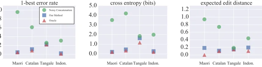
Figure 3: Results on the small phonological exercise datasets (≈100word types). Smaller numbers are better. Preliminary tests suggested that the variance of the prior (section 3.4) did not strongly affect the results, so we tookσ2_{= 5for all experiments.}

distributionbin terms ofPsb(s)L(s∗, s)whereL is unweighted Levenshtein distance.

We take the average of each measure over test words, weighting those words according top. This

yields our three reported metrics: 1-best error rate, cross-entropy, and expected edit distance. Each metric is the expected value of some mea-sure on a random test token.

These metrics are actually random variables, since they depend on the randomly sampled train-ing set and the resulttrain-ing test distribution. We re-port the expectations of these random variables by running many training-test splits (see section 7.2).

7.2 Datasets

To test discovery of interesting patterns from lim-ited data, we ran our learner on 5 “exercises” drawn from phonology textbooks (102 English nouns, 68 Maori verbs, 72 Catalan adjectives, 55 Tangale nouns, 44 Indonesian nouns), exhibiting a range of phenomena. In each case we tookpto

be the uniform distribution over the provided word types. We took N to be one less than the num-ber of provided types. So to report our expected metrics, we ran allN + 1experiments where we

trained jointly onN forms and tested on the 1

re-maining form. This is close to linguists’ practice of fitting an analysis on the entire dataset, yet it is a fair test. There is no sampling error in these reported results, hence no need for error bars.

To test on larger, naturally occurring datasets, we ran our learner on subsets of the CELEX database (Baayen et al., 1995), which provides surface phonological forms and token counts for German, Dutch, and English words. For each language, we constructed a coherent subcorpus of 1000 nouns and verbs, focusing on inflections with common phonological phenomena. These turned out to involve mainly voicing: final

obstru-ent devoicing (German 2nd-person presobstru-ent indica-tive verbs, German nominaindica-tive singular nouns, Dutch infinitive verbs, Dutch singular nouns) and voicing assimilation (English past tense verbs, En-glish plural nouns). We were restricted to rela-tively simple phenomena because our current rep-resentations are simple segmental strings that lack prosodic and autosegmental structure. In future we plan to consider stress, vowel harmony, and templatic morphology.

We constructed the distributionpin proportion

to CELEX’s token counts. In each language, we trained onN = 200, 400, 600, or 800 forms

sam-pled fromp. To estimate the expectation of each metric overalltraining sets of sizeN, we report the sample mean and bootstrap standard error over 10 random training sets of sizeN.

Except in Indonesian, every word happens to consist of≤2morphemes (a stem plus a possibly

empty suffix). In all cases, we take the phoneme inventoriesΣ_uandΣ_sto be given as the set of all surface phonemes that appear in the full dataset.

7.3 Comparison systems

There do not appear to be previous systems that perform our generalization task. Therefore, we compared our own system against variants.

We performed an ablation study to determine whether the learned phonology was helpful. We substituted a simplified phonology model where

Sθ(s | u)just decays exponentially with the edit distance between s and u; the decay rate was

learned by EM as usual. That is, this model uses onlythe COPYfeature of section 6. This baseline system treats phonology as “noisy concatenation” of learned URs, not trying to model its regularity.

0.00 0.05 0.10 0.15 0.20 0.25

1-best error rate

German

0.05 0.10 0.15 0.20 0.25

0.30

Dutch

0.00.1 0.2 0.3 0.40.5 0.6

0.7

English

0.0 0.5 1.0 1.5 2.0 2.5 3.0

cross-entropy (bits) _0.00.5 1.0 1.5 2.0 2.5 3.0

0.0 1.0 2.0 3.0 4.0 5.0 6.0

200 400 600 800 0.00

0.05 0.10 0.15 0.20 0.25 0.30

expected edit distance

200 400 600 800

0.05 0.10 0.15 0.20 0.25 0.30 0.35 0.40 0.45 0.50

200 400 600 800 0.0

0.2 0.4 0.6 0.8 1.0 1.2

Figure 4: Results on the CELEX datasets (1000 word types) at 4 different training set sizesN. The larger training sets are supersets of the smaller, obtained by continuing to sample without replacement fromp. For each training set, theunconnected points evaluate all words∈/training whose morphemes∈training. Meanwhile, theconnectedpoints permit comparison across the 4 values ofN, by evaluating only on a common test set found by intersecting the 4 unconnected test sets. Each point estimates the metric’s expectation overallways of sampling the 4 training sets; specifically, we plot thesample meanfrom 10 such runs, witherror barsshowing a bootstrap estimate of the standard error of the mean. Non-overlapping error bars at a given Nalways happen to imply that the difference in the two methods’ sample means is too extreme to be likely to have arisen by chance (paired permutation test,p <0.05). Each time we evaluated some training-test split on some metric, we first tunedσ2

(section 3.4) by a coarse grid search where we trained on the first 90% of the training set and evaluated on the remaining 10%.

heuristic for identifying URs in some simpler way. Thus, instead we asked whether the learned URs were as good as hand-constructed URs. Our “ora-cle” system was allowed to observe gold-standard URs for stems instead of inferring them. This system is still fallible: it must still infer the af-fix URs by belief propagation, and it must still use MAP-EM to estimate a phonology within our current model familySθ. Even with supervision, this family will still struggle to model many types of phonology, e.g., ablaut patterns (in Germanic strong verbs) and many stress-related phenomena.

7.4 Results

We graph our results in Figures 3 and 4. When given enough evidence, our method works quite well across the 7 datasets. For 94–98% of held-out words on the CELEX languages (whenN = 800), and 77–100% on the phonological exercises, our method’s top pick is the correct surface form. Fur-ther, the other metrics show that it places most of

Phon. Exercises CELEX

Maori 95.5 German 99.9

Catalan 99.5 Dutch 86.3

Tangale 79.8 English 82.2

Indonesian 100

Table 2: Percent of training words, weighted by the distribu-tionp, whose 1-best recovered UR (including the boundary #) exactly matches the manual “gold” analysis. Results are av-erages over all runs (withN = 800for the CELEX datasets).

its probability mass on that form,12_{and the rest on} highly similar forms. Notably, our method’s pre-dictions are nearly as good as if gold stem URs had been supplied (the “oracle” condition). Indeed, it doestend to recover those gold URs (Table 2).

Yet there are some residual errors in predict-ing the SRs. Our phonological learner cannot perfectly learn the UR-to-SR mapping even from many well-supervised pairs (the oracle condition). In the CELEX and Tangale datasets, this is partly 12_{Cross-entropy< 1bit means that the correct form has}

due to irregularity in the language itself. However, error analysis suggests we also miss some gener-alizations due to the imperfections of our current

Sθmodel (as discussed in sections 3.2 and 6). When given less evidence, our method’s per-formance is more sensitive to the training sample and is worse on average. This is expected: e.g., a stem’s final consonant cannot be reconstructed if it was devoiced (German) or deleted (Maori) inall the training SRs. However, a contributing factor may be the increased error rate of the phonolog-ical learner, visible even with oracle data. Thus, we suspect that aSθ model with better general-ization would improve our results at all training sizes. Note that weakening Sθ—allowing only “noisy concatenation”—clearly harms the method, proving the need for true phonological modeling.

8 Related Work

We must impute the inputs to the phonologi-cal noisy channelSθ (URs) because we observe only the outputs (SRs). Other NLP problems of this form include unsupervised text normalization (Yang and Eisenstein, 2013), unsupervised train-ing of HMMs (Christodoulopoulos et al., 2010), and particularly unsupervised lexicon acquisition from phonological data (Elsner et al., 2012). How-ever, unlike these studies, we currently use some indirect supervision—we know each SR’s mor-pheme sequence, though not the actual morphs.

Jarosz (2013,§2) and Tesar (2014, chapters 5– 6) review work on learning the phonology Sθ. Phonologists pioneered stochastic-gradient and passive-aggressive training methods—the Gradual Learning Algorithm (Boersma, 1998) and Error-Driven Constraint Demotion (Tesar and Smolen-sky, 1998)—for structured prediction of the sur-face wordsfrom the underlying wordu. Ifsis not

fully observed during training (layer 4 of Figure 1 is observed, not layer 3), then it can be imputed, a step known as Robust Interpretive Parsing.

Recent papers consider our setting whereu = m1#m2#· · · is not observed either. Thecontrast

analysismethod (Tesar, 2004; Merchant, 2008) in effect uses constraint propagation (Dechter, 2003). That is, it serially eliminates variable values (de-scribing aspects of the URs or the constraint rank-ing) that are provably incompatible with the data. Constraint propagation is an incomplete method that is not guaranteed to make all logical de-ductions. We use its probabilistic generalization,

loopy belief propagation (Dechter et al., 2010)— which is still approximate but can deal with noise and stochastic irregularity. A further improvement is that we work with string-valued variables, repre-senting uncertainty using WFSMs; this lets us rea-son about URs of unknown length and unknown alignment to the SRs. (Tesar and Merchant in-stead used binary variables, one for each segmen-tal feature in each UR—requiring the simplify-ing assumption that the URs are known except for their segmental features. They assume that SRs are annotated with morph boundaries and that the phonology only changes segmental features, never inserting or deleting segments.) On the other hand, Tesar and Merchant reason globally about the con-straint ranking, whereas in this paper, we only lo-cally improve the phonology—we use EM, rather than the full Bayesian approach that treats the pa-rameters_θ~_{as variables within BP.}

Jarosz (2006) is closest to our work in that she uses EM, just as we do, to maximize the probabil-ity of observed surface forms whose constituent morphemes (but not morphs) are known.13 _Her model is a probabilistic analogue of Apoussidou (2006), who uses a latent-variable structured per-ceptron. A non-standard aspect of this model (de-fended by Pater et al. (2012)) is that a morpheme

acan stochastically choosedifferentmorphsM(a)

when it appears in different words. To obtain a sin-gle shared morph, one could penalize this distribu-tion’s entropy, driving it toward 0 as learning pro-ceeds. Such an approach—which builds on a sug-gestion by Eisenstat (2009,§5.4)—would loosely resemble dual decomposition (Peng et al., 2015). Unlike our BP approach, it would maximize rather than marginalize over possible underlying morphs. Our work has focused on scaling up inference. For the phonologyS, the above papers learn the weights or rankings of just a few plausible con-straints (or Jarosz (2006) learns a discrete distribu-tion over all5! = 120rankings of 5 constraints),

whereas we use Sθ with roughly 50,000 con-straints (features) to enable learning of unknown languages. Our S also allows exceptions. The above papers also consider only very restricted sets of morphs, either identifying a small set of plausible morphs or prohibiting segmental inser-tion/deletion. We use finite-state methods so that it is possible to consider the spaceΣ∗_uof all strings.

13_{She still assumes that word SRs are annotated with}

On the other hand, we are divided from pre-vious work by our inability to use an OT gram-mar (Prince and Smolensky, 2004), a stochastic OT grammar (Boersma, 1997), or even a maxi-mum entropy grammar (Goldwater and Johnson, 2003; Dreyer et al., 2008; Eisenstat, 2009). The reason is that our BP methodinvertsthe phonolog-ical mappingSθto find possible word URs. Given a word SRs, we construct a WFSM (message) that

scores everypossible UR u _∈ Σ∗_u—the score of uis Sθ(s | u). For this to be possible without approximation,Sθ itself must be represented as a WFSM (section 3.2). Unfortunately, the WFSM for a maximum entropy grammar does not com-puteSθbut only an unnormalized version, with a different normalizing constantZuneeded foreach

u. We plan to confront this issue in future work.

In the NLP community, Elsner et al. (2013) re-sembles our work in many respects. Like us, they recover a latent underlying lexicon (using the same simple priorMφ) and use EM to learn a phonol-ogy (rather similar to ourSθ, though less power-ful).14 _{Unlike us, they do not assume annotation} of the (abstract) morpheme sequence, but jointly learn a nonparametric bigram model to discover the morphemes. Their evaluation is quite different, as their aim is actually to recover underlyingwords from phonemically transcribed child-directed En-glish utterances. However, nothing in their model distinguishes words from morphemes—indeed, sometimes they do find morphemes instead—so their model could be used in our task. For infer-ence, they invert the finite-stateSθlike us to recon-struct a lattice of possible UR strings. However, they do this not within BP but within a block Gibbs sampler that stochastically reanalyzes utterances one at a time. Whereas our BP tries to find a con-sensus UR for each given morpheme type, their sampler posits morph tokens while trying to reuse frequent morph types, which are interpreted as the morphemes. Withobservedmorphemes (our set-ting), this sampler would fail to mix.

Dreyer and Eisner (2009, 2011) like us used loopy BP and MAP-EM to predict morphologi-cal SRs. Their 2011 paper was also able to ex-ploit raw text without morphological supervision. However, they directly modeled pairwise finite-state relationships among thesurfaceword forms

14_{Elsner et al. (2012) used an S}

θ quite similar to ours though lacking bigram well-formedness features. Elsner et al. (2013) simplified this for efficiency, disallowing segmen-tal deletion and no longer modeling the context of changes.

without using URs. Their model is a joint distribu-tion overnvariables: the word SRs of a single

in-flectional paradigm. Since it requires a fixedn, it does not directly extend to derivational morphol-ogy: deriving new words would require adding new variables, which—for an undirected model like theirs—changes the partition function and re-quires retraining. By contrast, our traineddirected model is a productive phonological system that can generate unboundedly many new words (see section 4.1). By analogy,nsamples from a Gaus-sian would be described with a directed model, and inferring the Gaussian parameters predicts any number of future samplesn+ 1, n+ 2, . . ..

Bouchard-Cˆot´e et al., in several papers from 2007 through 2013, have used directed graphi-cal models over strings, like ours though without loops, to modeldiachronicsound change. Some-times they use belief propagation for inference (Hall and Klein, 2010). Their goal is to recover la-tenthistoricalforms (conceptually, surface forms) rather than latent underlying forms. The results are evaluated against manual reconstructions.

None of this work has segmented words into morphs, although Dreyer et al. (2008) did seg-ment surface words into latent “regions.” Creutz and Lagus (2005) and Goldsmith (2006) segment an unannotated collection of words into reusable morphs, but without modeling contextual sound change, i.e., phonology.

9 Conclusions and Future Work

We have laid out a probabilistic model for gener-ative phonology. This lets us infer likely expla-nations of a collection of morphologically related surface words, in terms of underlying morphs and productive phonological changes. We do so by ap-plying general algorithms for inference in graphi-cal models (improved in our followup papers: see section 4.4) and for MAP estimation from incom-plete data, using weighted finite-state machines to encode uncertainty. Throughout our presentation, we were careful to point out various limitations of our setup. But in each case, we also outlined how future work could address these limitationswithin the framework we propose here.

Acknowledgments

This material is based upon work supported by the National Science Foundation under Grant No. 1423276, and by a Fulbright grant to the first au-thor. The work was completed while the first author was visiting Ludwig Maximilian Univer-sity of Munich. For useful discussion of presen-tation, terminology, and related work, we would like to thank action editor Sharon Goldwater, the anonymous reviewers, Reut Tsarfaty, Frank Fer-raro, Darcey Riley, Christo Kirov, and John Sylak-Glassman.

References

Diana Apoussidou. 2006. On-line learning of under-lying forms. Technical Report ROA-835, Rutgers Optimality Archive.

R. Harald Baayen, Richard Piepenbrock, and Leon Gu-likers. 1995. The CELEX lexical database on CD-ROM.

Juliette Blevins. 1994. A phonological and morpho-logical reanalysis of the Maori passive. Te Reo, 37:29–53.

Paul Boersma and Bruce Hayes. 2001. Empirical tests of the Gradual Learning Algorithm. Linguistic In-quiry, 32(1):45–86.

Paul Boersma. 1997. How we learn variation, option-ality, and probability. InProceedings of the Institute of Phonetic Sciences of the University of Amsterdam, volume 21, pages 43–58.

Paul Boersma. 1998. How we learn variation, op-tionality, and probability. InFunctional Phonology: Formalizing the Interactions Between Articulatory and Perceptual Drives, chapter 15. Ph.D. Disserta-tion, University of Amsterdam. Previously appeared inIFA Proceedings(1997), pp. 43–58.

Alexandre Bouchard-Cˆot´e, Percy Liang, Thomas L. Griffiths, and Dan Klein. 2007. A probabilistic ap-proach to language change. InProceedings of NIPS. Alexandre Bouchard-Cˆot´e, David Hall, Thomas L. Griffiths, and Dan Klein. 2013. Automated re-construction of ancient languages using probabilis-tic models of sound change.Proceedings of the Na-tional Academy of Sciences.

Noam Chomsky and Morris Halle. 1968. The Sound Pattern of English. Harper and Row.

Christos Christodoulopoulos, Sharon Goldwater, and Mark Steedman. 2010. Two decades of unsuper-vised POS induction: How far have we come? In

Proceedings of EMNLP, pages 575–584.

George N. Clements and Elizabeth V. Hume. 1995. The internal organization of speech sounds. In John Goldsmith, editor,Handbook of Phonological The-ory. Oxford University Press, Oxford.

Ryan Cotterell and Jason Eisner. 2015. Penalized expectation propagation for graphical models over strings. InProceedings of NAACL-HLT, pages 932– 942, Denver, June. Supplementary material (11 pages) also available.

Ryan Cotterell, Nanyun Peng, and Jason Eisner. 2014. Stochastic contextual edit distance and probabilistic FSTs. InProceedings of ACL.

Mathias Creutz and Krista Lagus. 2005. Induc-ing the morphological lexicon of a natural lan-guage from unannotated text. InProceedings of the International and Interdisciplinary Conference on Adaptive Knowledge Representation and Reasoning (AKRR05), volume 1.

Rina Dechter, Bozhena Bidyuk, Robert Mateescu, and Emma Rollon. 2010. On the power of belief propagation: A constraint propagation per-spective. In Rina Dechter, Hector Geffner, and Joseph Y. Halpern, editors,Heuristics, Probability and Causality: A Tribute to Judea Pearl. College Publications.

Rina Dechter. 2003. Constraint Processing. Morgan Kaufmann.

Markus Dreyer and Jason Eisner. 2009. Graphical models over multiple strings. In Proceedings of EMNLP, pages 101–110.

Markus Dreyer and Jason Eisner. 2011. Discover-ing morphological paradigms from plain text usDiscover-ing a Dirichlet process mixture model. InProceedings of the Conference on Empirical Methods in Natu-ral Language Processing (EMNLP), pages 616–627, Edinburgh, July. Supplementary material (9 pages) also available.

Markus Dreyer, Jason R. Smith, and Jason Eisner. 2008. Latent-variable modeling of string transduc-tions with finite-state methods. In Proceedings of EMNLP, pages 1080–1089.

Markus Dreyer. 2011. A Non-Parametric Model for the Discovery of Inflectional Paradigms from Plain Text Using Graphical Models over Strings. Ph.D. thesis, Johns Hopkins University, Baltimore, MD, April.

Sarah Eisenstat. 2009. Learning underlying forms with MaxEnt. Master’s thesis, Brown University, Providence, RI.

Jason Eisner. 2002a. Comprehension and compilation in Optimality Theory. InProceedings of ACL, pages 56–63, Philadelphia, July.

Jason Eisner. 2015. Should linguists evaluate gram-mars or grammar learners? In preparation.

Micha Elsner, Sharon Goldwater, and Jacob Eisenstein. 2012. Bootstrapping a unified model of lexical and phonetic acquisition. InProceedings of ACL, pages 184–193.

Micha Elsner, Sharon Goldwater, Naomi Feldman, and Frank Wood. 2013. A joint learning model of word segmentation, lexical acquisition, and phonetic vari-ability. InProceedings of EMNLP, pages 42–54. Alexander M. Fraser, Marion Weller, Aoife Cahill, and

Fabienne Cap. 2012. Modeling inflection and word-formation in SMT. InProceedings of EACL, pages 664–674.

J. Goldsmith. 2006. An algorithm for the unsupervised learning of morphology. Natural Language Engi-neering, 12(4):353–371.

Sharon Goldwater and Mark Johnson. 2003. Learning OT constraint rankings using a maximum entropy model. In Jennifer Spenader, Anders Eriksson, and Osten Dahl, editors,Proceedings of the Workshop on Variation within Optimality Theory, pages 113–122, Stockholm University.

David Hall and Dan Klein. 2010. Finding cognate groups using phylogenies. InProceedings of ACL. Bruce Hayes and Colin Wilson. 2008. A maximum

en-tropy model of phonotactics and phonotactic learn-ing. Linguistic Inquiry, 39(3):379–440.

Matt Hohensee and Emily M. Bender. 2012. Getting more from morphology in multilingual dependency parsing. InProceedings of NAACL-HLT, pages 315– 326.

Mans Hulden. 2009. Revisiting multi-tape automata for Semitic morphological analysis and generation. In Proceedings of the EACL 2009 Workshop on Computational Approaches to Semitic Languages, pages 19–26, March.

Sharon Inkelas and Cheryl Zoll. 2005.Reduplication: Doubling in Morphology. Number 106 in Cam-bridge Studies in Linguistics. CamCam-bridge University Press.

Roman Jakobson. 1948. Russian conjugation. Word, 4:155–167.

Gaja Jarosz. 2006. Richness of the base and proba-bilistic unsupervised learning in Optimality Theory. InProceedings of the Eighth Meeting of the ACL Special Interest Group on Computational Phonology and Morphology, pages 50–59.

Gaja Jarosz. 2013. Learning with hidden structure in optimality theory and harmonic grammar: Beyond robust interpretive parsing. Phonology, 30(01):27– 71.

C. Douglas Johnson. 1972.Formal Aspects of Phono-logical Description. Mouton.

Ren´e Kager. 1999.Optimality Theory, volume 2. MIT Press.

Ronald M. Kaplan and Martin Kay. 1994. Regu-lar models of phonological rule systems. Compu-tational Linguistics, 20(3):331–378.

Michael J. Kenstowicz and Charles W. Kisseberth. 1979. Generative Phonology. Academic Press San Diego.

Andr´as Kornai. 1995. Formal Phonology. Garland Publishing, New York.

Zhifei Li and Jason Eisner. 2009. First- and second-order expectation semirings with applications to minimum-risk training on translation forests. In

Proceedings of EMNLP, pages 40–51, Singapore, August.

Dong C. Liu and Jorge Nocedal. 1989. On the limited memory BFGS method for large scale optimization.

Mathematical Programming, 45(1-3):503–528. Andrew McCallum, Dayne Freitag, and Fernando C. N.

Pereira. 2000. Maximum entropy Markov mod-els for information extraction and segmentation. In

Proceedings of ICML, pages 591–598.

Navarr´e Merchant. 2008. Discovering Underlying Forms: Contrast Pairs and Ranking. Ph.D. thesis, Rutgers University. Available on the Rutgers Opti-mality Archive as ROA-964.

Kevin P. Murphy, Yair Weiss, and Michael I. Jordan. 1999. Loopy belief propagation for approximate in-ference: An empirical study. InProceedings of UAI, pages 467–475.

Joe Pater, Karen Jesney, Robert Staubs, and Brian Smith. 2012. Learning probabilities over underly-ing representations. InProceedings of the Twelfth Meeting of the Special Interest Group on Computa-tional Morphology and Phonology, pages 62–71. Judea Pearl. 1988. Probabilistic Reasoning in

In-telligent Systems: Networks of Plausible Inference. Morgan Kaufmann Publishers Inc., San Francisco, CA, USA.

Nanyun Peng, Ryan Cotterell, and Jason Eisner. 2015. Dual decomposition inference for graphical models over strings. In Proceedings of EMNLP, Lisbon, September. To appear.

Janet Pierrehumbert. 2003. Probabilistic phonology: Discrimination and robustness. InProbabilistic Lin-guistics, pages 177–228. MIT Press.

Jason A. Riggle. 2004. Generation, Recognition, and Learning in Finite State Optimality Theory. Ph.D. thesis, University of California at Los Angeles.

Jason Riggle. 2012. Phonological features chart (version 12.12). Available online at https: //dl.dropboxusercontent.com/u/ 5956329/Riggle/PhonChart_v1212.pdf

(retrieved 2015-08-07).

David Sankoff. 1978. Probability and linguistic varia-tion.Synthese, 37(2):217–238.

Ferdinand de Saussure. 1916. Course in General Lin-guistics. Columbia University Press. English edi-tion of June 2011, based on the 1959 translaedi-tion by Wade Baskin.

Paul Smolensky and G´eraldine Legendre. 2006. The Harmonic Mind: From Neural Computation to Optimality-Theoretic Grammar (Vol. 1: Cognitive Architecture). MIT Press.

Bruce Tesar and Paul Smolensky. 1998. Learnability in Optimality theory.Linguistic Inquiry, 29(2):229– 268.

Bruce Tesar. 2004. Contrast analysis in phonological learning. Technical Report ROA-695, Rutgers Opti-mality Archive.

Bruce Tesar. 2014.Output-Driven Phonology: Theory and Learning. Cambridge University Press. Yi Yang and Jacob Eisenstein. 2013. A log-linear

model for unsupervised text normalization. In

EMNLP, pages 61–72.