LANKFORD, GEORGE BERNARD. Optimization, Modeling, and Control: Applications to Klystron Designing and Hepatitis C Virus Dynamics. (Under the direction of Dr. Hien Tran.)
In this dissertation, we address applying mathematical and numerical techniques in the fields of high energy physics and biomedical sciences. The first portion of this thesis presents a method for optimizing the design of klystron circuits. A klystron is an electron beam tube lined with cavities that emit resonant frequencies to velocity modulate electrons that pass through the tube. Radio frequencies (RF) inserted in the klystron are amplified due to the velocity modulation of the elec-trons. The routine described in this work automates the selection of cavity positions, resonant frequencies, quality factors, and other circuit parameters to maximize the efficiency with required gain. The method is based on deterministic sampling methods. We will describe the procedure and give several examples for both narrow and wide band klystrons, using the klystron codes AJDISK (Java) and TESLA (Python).
by
George Bernard Lankford
A dissertation submitted to the Graduate Faculty of North Carolina State University
in partial fulfillment of the requirements for the Degree of
Doctor of Philosophy
Applied Mathematics
Raleigh, North Carolina
2016
APPROVED BY:
Dr. Mansoor Haider Dr. Ralph Smith
Dr. Marina Evans Dr. Hien Tran
I dedicate this to Sharonda Hill-Stevens Porter. She isn’t perfect, but I know the large amount of love in her heart. She has endured so much and still will take anyone off the street into her home whether she likes you or not. She took me in, gave me a roof over my head and food in my mouth.
First and foremost, I would like to thank my advisor, Dr. Hien Tran. It is tough to really know how many times I popped in your office and went "You got a second Dr. T?" I am so grateful for all of the knowledge and assistance you have imparted to me these past five years. You made this process enjoyable and I am thankful to be your student.
I would like to also thank all of my committee members for their assistance in my journey. Dr. Evans and Dr. Haider, thank you for being supportive of me during this process. Dr. Smith, I am so appreciative for your kindness over the years. You were one of the first professors that I met when I got here. Countless times we’ve met in the hall at SAS and warmheartedly you would say, "George, how’s it going?" Thank you for being a welcoming smile.
There are too many coaches, teachers, and professors that I want to put here, however, I want to point out a couple. I want to acknowledge my wrestling coach Bengie Balentine and my advisor, Dr. William Yin and his family. Thank you for your endless support and encouraging words through this process.
To President Linda Buchanan, Tom and Pandora Economy, and Charles and Jeannie Smith, I love you all so very much. You and your families have been there for me when I needed you during my journey and I can’t thank you enough.
I acknowledge all of my family, the Lankfords, the Johnsons, the Porters, and whomever else has been like family to me. I’m grateful for your support during my journey. Special thanks to all my friends like Bill Simons and Kaska Adoteye who have been there for me since the beginning of graduate school. Also, shoutout to Emaan Abdul-Majid, Joshua Richardson, and Zach Hough for your encouraging words and enduring my stories of weekly crying at the end of my tenure as a graduate student.
LIST OF TABLES . . . vii
LIST OF FIGURES. . . .viii
Chapter 1 INTRODUCTION . . . 1
1.1 Thesis Outline . . . 2
1.2 Optimization Techniques . . . 2
1.2.1 Unconstrained and Constrained Minimization . . . 3
1.2.2 Gradient Based Methods . . . 4
1.2.3 Non-Gradient Based Methods . . . 9
1.3 Modeling Techniques and Validation . . . 15
1.3.1 Sensitivity Analysis . . . 16
1.3.2 Identifiability Analysis . . . 24
1.3.3 Data Analysis . . . 26
1.3.4 Confidence and Prediction Intervals . . . 29
Chapter 2 Optimization of Klystron Designs Using Deterministic Sampling Methods . . . 35
2.1 Introduction . . . 35
2.2 Methodology . . . 38
2.2.1 Deterministic Sampling Methods . . . 38
2.2.2 Simulation Programs . . . 38
2.2.3 Optimizer Scheme . . . 40
2.3 Examples . . . 42
2.3.1 CBAND . . . 42
2.3.2 KSB . . . 44
2.4 Discussion . . . 46
2.5 Conclusion . . . 46
Chapter 3 Mathematical Model of Hepatitis C Virus . . . 47
3.1 Introduction . . . 47
3.2 Model . . . 49
3.2.1 Motivation . . . 49
3.2.2 Assumptions . . . 50
3.2.3 Model from Snoeck et. al. . . 50
3.2.4 Model with DAA . . . 52
3.2.5 Existence and Uniqueness . . . 53
3.2.6 Steady States and Stability . . . 55
3.2.7 Treatment Schedule . . . 57
3.3 Subset Selection . . . 58
3.3.1 Fixed Parameters . . . 58
3.3.2 Sensitivity Analysis Model Considerations and Results . . . 59
3.5 Conclusion . . . 68
Chapter 4 Immune Response and Control. . . 69
4.1 Introduction . . . 69
4.2 Immune Response . . . 70
4.2.1 Innate Immune Response . . . 70
4.2.2 Adaptive Response . . . 70
4.3 Model . . . 72
4.3.1 Existence and Uniqueness . . . 72
4.3.2 Steady States and Stability . . . 72
4.4 Subset Selection . . . 74
4.4.1 Sensitivity Analysis Results . . . 76
4.4.2 Identifiability Analysis Results . . . 77
4.5 Parameter Estimation . . . 77
4.5.1 Discussion . . . 80
4.5.2 Akaike Information Criteria . . . 80
4.6 Control . . . 82
4.6.1 Control Formulation . . . 82
4.6.2 Subperiod Method . . . 83
4.6.3 Numerical Simulations . . . 84
4.7 Conclusion . . . 93
Chapter 5 Conclusion and Future Work . . . 94
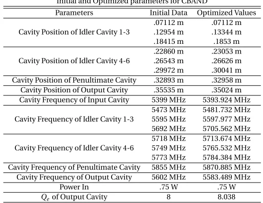
Table 2.1 Initial and optimized parameter values for the CBAND klystron. . . 43
Table 2.2 Initial and optimized parameter values for design one of the KSB klystron. . . 45
Table 2.3 Initial and optimized parameter values for design two of the KSB klystron. . . 45
Table 3.1 Typical values from[95]. . . 52
Table 3.2 Steady state values for (3.5). . . 56
Table 3.3 Patient ETR’s RBV efficacies based on modified dosage. . . 63
Table 3.4 Fixed parameter values from[95]and[5]. . . 65
Table 3.5 Values from parameter estimation for (3.5). . . 67
Table 4.1 Steady state values using PVR parameters. . . 73
Table 4.2 Steady state values using ETR parameters. . . 74
Table 4.3 Steady state values using Breakthrough parameters. . . 74
Table 4.4 Values from parameter estimation for (4.1). . . 78
Table 4.5 The AIC scores for (3.5) and (4.1) for each patient behavior. . . 81
Figure 1.1 A simplex and points considered during the Nelder-Mead algorithm from[37]. . 12
Figure 1.2 A graph of the different simplexes associated with the implementation of the Nelder-Mead algorithm where each triangle is a simplex and the minimum at p= (3, 2). . . 12
Figure 1.3 The implicit filtering iterations are able to skip many local minima. . . 15
Figure 1.4 Solution to (1.19) withK =10,r =1 andx0=.1. . . 21
Figure 1.5 Graphs show a comparison of sensitivities using the sensitivity equations with automatic differentiation, central difference, and complex step methods with withh=1×10⁻¹⁰. . . 22
Figure 1.6 Graphs show a comparison of sensitivities using the sensitivity equations with automatic differentiation, central difference, and complex step methods with withh=1×10−200. . . 23
Figure 1.7 Viral load pattern for a Breakthrough patient. . . 26
Figure 2.1 Diagram of a Klystron from[99]. . . 36
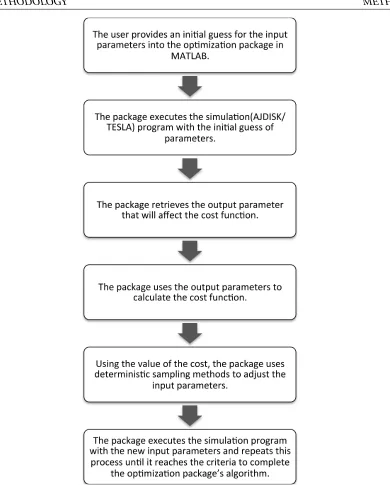
Figure 2.2 Schematic diagram for the local optimizer routine. . . 41
Figure 2.3 The Gain (left) and The Power Out (right) for CBAND with a run time of approx-imately 38 hours. . . 43
Figure 3.1 Simulation of (3.5) with initial conditions[T0,I0,VI0] = [1.92×10⁷, 0, 1]. . . 57
Figure 3.2 Treatment schedule for patients used for data received from patients treated at University of Sao Paulo, School of Medicine in Sao Paulo, Brazil. . . 57
Figure 3.3 Sensitivity rankings using PVR time points. . . 61
Figure 3.4 Sensitivity rankings using Breakthrough time points. . . 61
Figure 3.5 Final subset percentages using PVR time points. . . 62
Figure 3.6 Final subset percentages using Breakthrough time points. . . 63
Figure 3.7 Examples of viral load profiles for PVR, ETR, and Breakthrough patients. . . 64
Figure 3.8 Results from parameter estimation for (3.5). . . 66
Figure 3.9 Predictive confidence intervals and prediction intervals for (3.5). . . 67
Figure 4.1 Simulation of (4.1) with initial conditions[T0,I0,VI0,E0] = [1.142×10⁵, 2×10⁴, 2.403× 10⁵, 5]and using parameter values used in Table 4.3. . . 75
Figure 4.2 Sensitivity rankings using PVR time points. . . 76
Figure 4.3 Sensitivity rankings using Breakthrough time points. . . 77
Figure 4.4 Final subset percentages using PVR time points. . . 78
Figure 4.5 Final subset percentages using Breakthrough time points. . . 78
Figure 4.6 Results from parameter estimation for (4.1). . . 79
Figure 4.7 Predictive confidence intervals and prediction intervals for (4.1). . . 80
Figure 4.8 Immune response for Breakthrough patient. . . 81
Figure 4.11 The weights for this implementation of the subperiod method on the PVR patient are{WV,Wε,Wγρ,WE}= [.001, 1, 1, 100]. . . 88 Figure 4.12 The weights for this implementation of the subperiod method on the
break-through patient are{WV,Wε,Wγρ,WE}= [1, 0, 0, 1] . . . 89 Figure 4.13 The weights for this implementation of the subperiod method on the
break-through patient are{WV,Wε,Wγρ,WE}= [10, 1, 1, 1] . . . 90 Figure 4.14 The weights for this implementation of the subperiod method on the
break-through patient are{WV,Wε,Wγρ,WE}= [.001, 1, 1, 100] . . . 91 Figure 4.15 The weights for this implementation of the subperiod method on the ETR
1
INTRODUCTION
The groundwork for mathematics is founded upon solving problems. Around 200 B.C., an ancient Chinese book calledChiu-chang Suan-shu(Nine Chapters on Arithmetic)was written. At the begin-ning of Chapter VIII, the following problem is given:
Three sheafs of a good crop, two sheafs of a mediocre crop, and
one sheaf of a bad crop are sold for 39 dou. Two sheafs of good, three mediocre, and one bad are sold for 34 dou; and one
good, two mediocre, and three bad are sold for 26 dou. What is
the price received for each sheaf of a good crop, each sheaf of a mediocre crop, and each sheaf of a bad crop?
This problem can subsequently be formulated as the system of linear equations given in (1.1):
3x+2y +z=39, 2x+3y +z=34,
x+2y +3z=26,
(1.1)
solve such a problem. One approach involves methodically eliminating variables by adding and/or subtracting multiples of the equations from each other. Another is by putting the coefficients into an augmented matrix and using Gaussian elimination. Indeed, solving problems is a catalyst for many branches of mathematics. However, certain problems may not always be understood in the physical sense. To this extent, people with a combination of mathematics and specialized knowledge are needed to bridge the gap between theory and applications. The foundation of applied mathematics involves studying methodology in mathematics, and using those methods to quantify and/or solve practical problems. This thesis concerns itself with furthering the field of applied mathematics by exploring how different mathematical techniques can be used to investigate real-world applications concerning klystron design and viral kinetic modeling.
1.1
Thesis Outline
The remainder of this chapter is dedicated to developing certain techniques in optimization and modeling that will be relevant to our study. The implementation of the aforementioned techniques with applications to beam tube design optimization and biological modeling is described in the remaining chapters. In Chapter 2, an automated algorithm is presented to improve klystron design. Chapter 3 is dedicated to developing and validating a new model for hepatitis C dynamics with triple drug therapy. In Chapter 4, the model in Chapter 3 is further developed to include an immune response dynamic and a control is used to investigate potential optimal drug treatment protocols. A summary and conclusion is given in Chapter 5.
1.2
Optimization Techniques
Most students initially learn about a special relation between two sets–usually denoted as aninput
price-revenue function, the maximum revenue may be a critical value. In the latter example, the point for which the object is at its lowest height on the surface may be at a critical value. Finding these values is such an important concept, that an entire branch of mathematics was built around solving such a problem. Indeed, the process of finding the minimum or maximum value of a function is calledoptimization. In what follows, we detail some of the optimization tools that will be used to help solve the problems developed in this thesis.
1.2.1 Unconstrained and Constrained Minimization
Given an objective functionJ :X⊂Rn→R, unconstrained minimization is the process of finding
the elementω∗such that
J(ω∗)≤J(ω)∀ω∈X, and is commonly denoted by
min ω J(ω).
Hereω∗is called the global minimizer of the function J. However, as noted in[61], this problem is considerably more difficult than finding the local minimizerω∗
J(ω∗)≤J(ω)∀ωnearω∗.
To quantify the meaning of near, we require the existence of anε >0 so that|ω∗−ω|< ε. The main difference between a constrained minimization problem and an unconstrained minimization problem is that the former problem involves conditions that must be enforced on the function’s output or input. Thus, instead of usingX,the entire domain ofJ, a setΩ⊂X such that the constraints hold is considered. Similarly, the global and local minimizers overΩare given as theω∗such that
J(ω∗)≤J(ω)∀ω∈Ω, and
J(ω∗)≤J(ω)∀ωnearω∗,
respectively. Depending on what is known aboutJ, there are many different methods that can be used to findω∗for both constrained and unconstrained minimization problems.
squared errors between our data and model output. To this end, one of our goals is to minimize objective functions of the form
J(t,p) =wi N
X
i=1
(yi−yˆ(ti,p))2,
wherewi∈Rare the weights,p∈Rm is the vector ofmparameters,yiis the measured data at time,
ti, and ˆy(ti;p)is the model output. The upcoming sections will introduce the methods used in this work following similar notation and theory given in[57, 61]and references therein.
1.2.2 Gradient Based Methods
One popular strategy for locating the local and/or absolute extrema of a function,f(x)forx∈R,
involves using derivatives. The derivative of a function,f0, exists if and only iff is sufficiently smooth. Recalling thatf0can be interpreted as the slope of the tangent line to the curve off at a given point, we observe that local extrema can only occur atxwhen f0(x) =0 for functions of this type. After finding these values, the second derivative,f00, is used to determine if that point is a local or absolute extrema. Iff0(x) =0 andf00(x)>0 thenf has a local minimum atx. Gradient based methods seek to extend this concept to functions of multiple variables so thatx∈Rn. The gradient of a function,∇f,
contains the partial derivatives with respect toxi, theith component ofx. We assume thatf is twice continuously differentiable (i.e.∇2f(x)exist) in order to consider gradient based methods. This is
because, as in the one dimensional case,∇f(x) =0 and||∇2f(x)||>0 is needed to guarantee a local minimum atx. Specific details about many other iterative gradient based optimization methods such as the conjugate gradient method, Newton’s method and the method of steepest descent can be found in[23, 40, 57, 61]. In what follows, we provide a comprehensive description of the method that was used in this thesis.
1.2.2.1 Levenberg-Marquardt Method
An important class of gradient based iterative strategies for optimization is the trust region approach. Letf :Rn→Rbe the considered function that is to be minimized. Given that f can be represented
by the quadratic model in (1.2)
mc(x) =f(xc) +∇f(xc)T(x−xc) +
(x−xc)THc(x−xc)
in some region, the idea is that (1.2) can be iteratively minimized in varying regions to ultimately determine the minimum off. HereHc is the matrix of partial derivatives
(∇2f)i j= ∂ 2f
∂xi∂xj ,
called the function hessian andxc is the center of a ball,B, known as thetrust regionsuch that
B(r) ={x| ||x−xc|| ≤r},
withtrust radius,r. The difference betweenxc and the minimum ofmc isst and thetrust region
problemis given by
min
||s||<rmc(xc+s). (1.3) At each iteration, the trial step,st, or the trial solution,xt=xc+st, is accepted as the solution to (1.3) and determines if the step and/orr should be revised. Let theactual reductioninf be given by
a r e d=f(xc)−f(xt).
The decrease in the quadratic model is given by
p r e d= mc(xc)−mc(xt),
= f(xc) +∇f(xc)T(xc−xc) +
(xc−xc)THc(xc−xc)
2 ,
−(f(xc) +∇f(xc)T(xt−xc) +
(xt−xc)THc(xt−xc)
2 ),
= − ∇f(xc)T(xc+st−xc)−(xc+st−xc)
TH
c(xc+st−xc)
2 ,
= − ∇f(xc)Tst −
sT t Hcst
2 ,
and is called thepredicted reductionsuch thatp r e d>0 unless∇f(xc) =0. Typically, three control parameters
µ0≤µ1< µ2,
determine if the trial step or trust region radius should be adjusted. Ifp r e da r e d < µ0,st is rejected. If a r e d
p r e d > µ2, thenr increases to ˆr =ω2·r whereω2>1. If a r e d
doesn’t expand infinitely, a bound for the lengthening ofr is set so that
r ≤c||∇f(xc)||,
for somec >0 that may depend on xc. Adjustment patterns such as a sufficient decrease in f being the factor that determines modifications tost or using |p r e d||∇−fa r e d|| | instead of a r e dp r e d can be implemented depending on the algorithm. A significant advantage of using the trust region approach is that there is an exact solution to (1.3). In what follows we prove the existence of an exact solution similar to what is given in[61, 96].
Theorem 1.2.1 Let g ∈Rnand let A be a symmetric N×N matrix. Let
m(s) =gTs+s
TAs
2 .
A vector s is a solution to
min
||s||≤rm(s), (1.4)
if and only if there is v≥0such that
(A+v I)s=−g,
and either v=0or||s||=r .
Proof 1.2.2 Consider the equivalent problem to (1.4) given by (1.5):
min
||s||2≤r2m(s). (1.5) Using the theory of Lagrange multipliers, where
F(s) =||s||2−r2, =sTs−r2,
if s solves (1.5) then it must also solve
∇m(s) =λ¯(∇F(s)),
g+As=λ¯(2s), (A+λI)s=−g,
(1.6)
subject to
Hereλ≥0is a multiple of the Lagrange multiplier associated with||s||2≤r2,λˆ. If s6=0and solves (1.4) then it also solves
min
||w||≤||s||m(w), (1.7)
because||w|| ≤ ||s|| ≤r . This means that for any w so that||w||=||s||, if (1.4) and (1.6) are combined then the following is obtained
−sT(A+λI)w+w
TAw
2 ≥ −s
T(A+λI)s+sTAs 2 , =⇒ −sTAw−λsTw+w
TAw
2 ≥ −s TAs
−λsTs+s
TAs
2 , =⇒ w
TAw
2 −s TAw
−λsTw+s
TAs
2 +
λsTs
2 ≥ −
λsTs
2 .
The following equalities
sTAw =s
TAw
2 +
wTAs
2 ,
λsTw =λs
Tw
2 +
λwTs
2 ,
are used after addingλw2Tw to both sides to give the following inequality
wTAw
2 −
sTAw
2 −
wTAs
2 −
λsTw
2 −
λwTs
2 +
sTAs
2 +
λsTs
2 +
λwTw
2 ≥
λwTw
2 −
λsTs
2 .
Therefore,
1 2(w−s)
T(A+λI)(w
−s)≥λ
2(w Tw
−sTs) =0. (1.8)
It follows from (1.8) that A+λI is positive semidefinite. If s=0, then g=0and s solves
min ||s||≤r
sTAs 2 ,
which implies A is positive semidefinite. Therefore, A+λI is always at least positive semidefinite since λ≥0. If s solves (1.6) and (1.7) then for any w
gTw+w
T(A+λI)w
2 ≥g
Ts+sT(A+λI)s 2 =⇒ m(w)≥m(s) +λ
2(s Ts
−wTw).
(1.9)
1. Ifλ=0and||s|| ≤r then s solves (1.4).
2. If||s||=r then s solves
m(s) = min ||w||=rm(w).
3. Ifλ≥0and||s||=r then s solves (1.4).
This completes the proof.
When positive definiteness is obtained for(A+λI)andw6=sthen the inequality is strict in (1.9) and
s=−(Hc+λI)−1g,
is the exact solution to (1.3). Levenberg-Marquardt algorithm[65, 69]takes advantage of adjustingλ instead ofr with respect top r e da r e d in their trust region based algorithm. Variations of this method can be found in[57, 96]but this work focuses on the algorithm as described in[61]. The Levenberg-Marquardt quadratic model with parameterλc at the pointxc is
m(x) =f(xc) + (x−xc)TR0(xc)TR(xc) + 1
2(x−xc) T(R0(x
c)TR0(xc) +λcI)(x−xc),
using the least squares objective function given by
f(x) =1
2 M
X
i=1
||ri(x)||22=1
2R(x) TR(x).
The minimizer ofm(x)is given by
xt=xc−(R0(xc)TR0(xc) +λcI)−1R0(xc)TR(xc), (1.10)
with steps=xt−xc. The predicted reduction is then
p r e d=m(xc)−m(xt),
=−sTR0(xc)TR(xc)− 1 2s
T(R0(x
c)TR0(xc) +λcI)s, =−sTR0(xc)TR(xc) +1
2s TR0(x
c)TR(xc)using (1.10), =−1
2s T
This means we will accept/reject our trial point,xt, and Levenberg-Marquardt parameter,λc, based on the ratio
a r e d p r e d =
f(xc)−f(xt)
m(xc)−m(xt),
=−2f(xc)−f(xt)
sT∇f(x c)
.
Adjustingλis opposite to how we adjustedr. Ifa r e dp r e d is large, the actual reduction in the function could be large. Thus,s should be large in order to go further in this direction, soλis decreased so that the term(R0(x
c)TR0(xc) +λcI)−1R0(xc)TR(xc)is larger in (1.10). By similar reasoning, ifa r e dp r e d is small,λincreases. This method converges q-quadratically[61]in the following sense
Definition Let{xn} ⊂Rnandx∗∈Rn.xn→x∗q-quadratically ifxn→x∗and there isK >0 such that
||xn+1−x∗|| ≤K||xn−x∗||2.
We use the MATLAB implementation in the packagenlinfitof algorithm (1.1).
Algorithm 1.1lmalg(x,R,kmax)
1. Setλ=λ0.
2. Fork=1, ...,k m a x
(a) Letxc=x.
(b) ComputeR, f,R0, and∇f; test for termination. (c) Computext using (1.10).
(d) Calllmfunc(xc,xt,x,f,λ) (see algorithm 1.2)
1.2.3 Non-Gradient Based Methods
Algorithm 1.2lmfunc(xc,xt,x+,f,λ)
1. z =xc
2. Do whilez=xc
(a) a r e d=f(xc)−f(xt),st =xt−xc,p r e d=−∇f(xc)
Ts t
2 .
(b) Ifa r e dp r e d < µ0then setz =xc,λ=max(ω2λ,λ0), and recompute the trial point with the new value ofλ.
(c) Ifµ0≤a r e dp r e d < µ1, then setz=xt andλ=max(ω2λ,λ0). (d) Ifµ1≤a r e dp r e d, then setz =xt.
Ifµ2<a r e dp r e d, then setλ=ω1λ. Ifλ < λ0, then setλ=0.
3. x+=z
with no knowledge of the gradient; however, some convergence criterion have been proven for specific functions in lower dimensions[31, 64]. An interesting class of these methods are called genetic algorithms. They are adaptive heuristic search algorithms that at each iteration mimics the principles of natural selection and genetics. Popularly used for mixed integer optimization, they use the initial population as “parents" and use them to give “offspring" based on their fitness score to move towards a minimum. The chief operators for these types of algorithms use probabilistic rather than deterministic transitions and are given in the following:
1. Reproduction- determines which of the parents are going to survive to the next generation.
2. Crossover- determines how the parents will be combined to make offspring.
3. Mutation- determines how changes will be made to parents to create offspring.
We refer the reader to[38, 48]and references therein for a more detailed description. The class of non-gradient based methods that are employed in this work are called deterministic sampling methods.
1.2.3.1 Deterministic Sampling Methods
search next for the optimal value of the objective function. Deterministic sampling methods use patterns to optimally guide the search[103]. There are a myriad of algorithms that use deterministic sampling like the Hooke-Jeeves algorithm and the multidirectional search method described in[61]. We describe two specific methods that are used in this research.
1.2.3.1.1 Nelder-Mead Algorithm
The Nelder-Mead algorithm is a non-gradient based method that is simplex based[61, 80]. Let
J :Rn→RandS={λ0,λ1,· · ·,λn}be a simplex ofn+1 points withλi∈Rn. We let
J(λl) =min λ∈S J(λ), and
J(λu) =max λ∈S J(λ).
By adjusting the point in the simplex that gives the value farthest from the objective, we are able to find the minimum over the space. Figure 1.1 gives a sketch of the simplex points (λ1,λ2,λ3) in two dimensions as well as the points considered to revise the simplex which are given by
• extension point (e),
• reflection point (r),
• outer contraction point (o c), and
Figure 1.1A simplex and points considered during the Nelder-Mead algorithm from[37].
Algorithm (1.3), as obtained from[37, 66, 74], gives a brief overview of how the Nelder-Mead algo-rithm is implemented. The tolerance between values of the functions and total number of iterations are among options for stopping criterion.
Figure 1.2 shows the first 11 iterations of the Nelder-Mead algorithm converging to the local mini-mum for a function of two variables.
Algorithm 1.3
1. Not includingλu, compute the centroid of the simplex,c,
c=
n
X
i=0,i6=u
λi
n .
2. Usingα=1 as the step size in the direction (in relevance to the centroid) that is opposite to the direction ofλu, calculate the reflection pointr =c+α(c−λu). IfJ(λl)≤J(r)<J(λk)where
J(λk)is the second lowest objective function value thenλuis replaced withr and restart.
3. Compute the extension pointe =c+α(c−su)whereα=2 ifJ(r)<J(λl)to expand the search further thanr. IfJ(e)<J(r),λuis replaced withe and the algorithm is restarted. If not, then the simplex is not expanded andλuis replaced withr and restart.
4. If the above is not true then check if J(r)≥J(λi)fori6=u. For this case, one of the following points are considered:
(a) IfJ(r)<J(λu)then the outer contraction point,o c =c+α(r−c), is computed where
α=1
2. IfJ(o c)<J(r)then replaceλuwitho c and restart.
(b) IfJ(r)≥J(λu)then the inner contraction point,i c =c+α(λu−c), is computed where
α=1
2. IfJ(i c)<J(λu)then replaceλu withi c and restart.
Convergence is only guaranteed in one dimension for strictly convex functions with bounded level sets[64]. In MATLAB, the optimization packagefminsearchprovides a numerical implementa-tion of the algorithm.
1.2.3.1.2 Implicit Filtering
Implicit filtering is a non-gradient based optimization routine that estimates the gradient using difference approximations[61]. The size of the increment in the difference varies as iterations progress. This is to filter out initial oscillations and circumvent local minima. Algorithm (1.4) gives a simplified version of the implicit filtering routine as described in[66]. The implicit filtering iterative
Algorithm 1.4
1. We start with the current minimum ofJ being atsc and initial step sizehc. A 2ndimensional stencil is created aboutsc and is given by
S(sc,hc) ={sc±hcei},
whereeiare unit vectors.
2. We then evaluate J at all points inS and let
J(su) =min{J(z)|z∈S(sc,hc)}.
3. Sets0=sc and let
sc=s0−λ∇hcJ(s0),
ifJ(su)<J(sc)whereλassures enough decrease such that
J(sc−λd)<J(sc)whered =−∇J(sc),
and
(∇hcJ(x))i=
J(x+hcei)−J(x−hcei) 2hc
.
4. If the above is not true and J(su)≥J(sc)thenhc is reduced and restart from step 1.
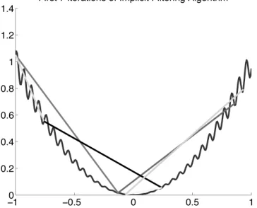
Figure 1.3 depicts a function where there are many local minima close together and the first 7 iterations of the implicit filtering algorithm trying to find the global minimum. It is noted that the algorithm initially uses a large step sizehc to avoid the many local minima.
Figure 1.3The implicit filtering iterations are able to skip many local minima.
In[31], the authors proved that if the objective function is smooth with low amplitude noise and the noise decays rapidly near the minimizer sufficiently, then superlinear convergence is established in the following sense
Definition Let{xn} ⊂Rn andx∗∈Rn.xn→x∗q-superlinearly if
lim n→∞
||xn+1−x∗||
||xn−x∗|| = 0.
1.3
Modeling Techniques and Validation
In Chapter 3, a system of nonlinear ordinary differential equations(ODEs) is used to model a biolog-ical phenomena. This means there are parameters in the model that are used to describe particular aspects of the system. Thus, emphasis should be placed in obtaining accurate estimates of these parameters while fitting model output to clinical data. These estimates can help determine the robustness and capabilities of the model in solving theforward problem. Theforward problem
refers to using a model to predict the future behavior of a system given a set of parameters. The
the parameters directly determines the accuracy of the model output. However, depending on the complexity of the model, providing accurate parameters can be challenging or impossible. There has been extensive study about parameter selection while solving the inverse problem for biological models and other applications that can be found in[5, 9, 11, 13, 14]and references therein. In what follows, we provide background for the techniques used to calibrate the parameters for the models used in this thesis.
1.3.1 Sensitivity Analysis
A sensitivity analysis is the process of understanding how the model output is affected by changes in the parameters. Sensitivity analyses are used in many branches of mathematics such as statistics, PDEs (partial differential equations), and control design[10, 106]. The parameters that give the most change in the output are said to be sensitive parameters. This is important in theforward problem
because it allows an understanding of which parameters will give useful information. Once the parameters have been identified, a sensitivity analysis for theinverse problemis usually performed to determine the sensitive parameters. Parameters with minimal impact are fixed from literature. There are two different types of sensitivity analysis: global and local. A global sensitivity analysis heavily depends on the structure of the model and quantifies how uncertainties in outputs can be apportioned to uncertainties in inputs. We refer the reader to[94]for more information. Our work uses a local sensitivity analysis which depends on the prescribed value of the parameters.
1.3.1.1 Sensitivity Equations
The sensitivity analysis presented in this section uses a derivative-based approach. Consider the general form of an ODE model and a functionz of its output
d y
d t =f(t,y;q), z=g(t,y;q),
(1.11)
partial derivative is by solving the associated sensitivity equations. Consider the formulation
∂z ∂q =
∂g ∂t
∂t ∂q +
∂g ∂y
∂y ∂q +
∂g ∂q,
∂q ∂q
=∂g
∂y ∂y ∂q +
∂g ∂q,
(1.12)
since∂∂qt =0 and∂∂qq =1. The two components ∂∂gy and ∂∂gq can be directly calculated fromg, but can be cumbersome to do by hand depending on the complexity of the function. Thus, one can employ automatic differentiation to evaluate these derivatives. Since any mathematical function can be decomposed into elementary functions, automatic differentiation numerically implements the chain rule and basic arithmetic equations repeatedly to compute the total derivative of a function with accuracy to working machine precision[25]. This is achieved with table lookups and tabulating all of the functional compositions[51, 73]. An automatic differentiation(AD) code developed by Martin Fink in MATLAB is employed. Finally, to calculate∂∂qy, it is noted thaty is continuous int
andq. Since∂∂qy exists, by computing the partial derivative with respect toqof the state equations and reversing the order of differentiation[100]the following is obtained
∂ ∂q
d y
d t
= d
d t ∂y
∂q
=∂f
∂t ∂t ∂q+
∂f ∂y
∂y ∂q +
∂f ∂q
∂q ∂q
=∂f
∂y ∂y ∂q +
∂f ∂q.
(1.13)
Similar to ∂∂gy and ∂∂gq, ∂∂fy and ∂∂qf is calculated using automatic differentiation. From (1.13), the sensitivity equations are given as follows
d y
d t =f(t,y;q), d
d t ∂y
∂q
=∂f
∂q ∂y ∂q +
∂f ∂q.
(1.14)
1.3.1.2 Finite Difference Approximation
A direct approach to findingd qd z
i is by a finite difference approximation whereqiis theith component
ofq. Recall by the definition of a derivative,
d z d qi
=lim h→0
z(qi+h)−z(qi)
h .
Thus, an approximation for the first derivative is the forward-difference formula given by
d z d qi ≈
z(qi+h)−z(qi)
h ,
with step size,h, andO(h)truncation error so it is accurate to first order. Another approximation for the first derivative is the backwards-difference formula given by
d z d qi ≈
z(qi)−z(qi−h)
h ,
that also hasO(h)truncation error. Adding the previous two formulas together yields the centered difference formula
2d z
d qi ≈
z(qi+h)−z(qi) +z(qi)−z(qi−h)
h ,
=⇒ d z d qi ≈
z(qi+h)−z(qi−h)
2h ,
(1.15)
and hasO(h2)truncation error so it is accurate to second order. The step size should be chosen to minimize truncation error and subtractive cancellation error due to finite precision arithmetic. In[57], it is shown that a good candidate for the step size in the backwards and forward differences ish =pmacheps·qi andh = (macheps)
1
3 ·qi for central difference where macheps is accuracy
at which the functionz is evaluated. Therefore, to obtain an accurate approximation to the finite difference of the derivative ofz,zmust be evaluated at high precision. A routine where subtractive cancellation error does not occur is preferable and is presented in the next section.
1.3.1.3 Complex Step Method
and Im(z)=y such that
f(z) =u(x+i y) +i v(x+i y)
is an analytic complex function whereuandvare the real and imaginary parts off, respectively. Sincef is analytic, it satisfies the Cauchy-Riemann equations. That is, the components satisfy
ux=vy, uy =−vx. (1.16)
The forward difference approximation is used to rewrite the first equation in (1.16) as
ux≈v(x+i(y+h))−v(x+i y)
h .
If the function is restricted to the real axis then the following are true:
y = 0,
v(x) = 0,
f(x) = u(x).
(1.17)
This implies that
d f
d x = ux,
≈ v(x+i h)−v(x)
h ,
= v(x+i h)
h .
(1.18)
Therefore, an approximation of the first derivative off at a given parameterxis
d f d x ≈
Im(f(x+i h))
h ,
and is called the complex step derivative approximation. This has an obvious advantage over the finite difference approximation because there is no subtraction operation and thus has no subtrac-tive cancellation error. The benefit over automatic differentiation is that it is usually quicker and uses less memory since it doesn’t take multiple function evaluations. We implement this method in MATLAB by evaluating f(x+i h)and recovering the imaginary component of the output overh.
Taylor series expansion is obtained about a real pointx,
f(x+i h) =f(x) +i h f0(x)−h2f
00(x) 2! −i h
3f000(x)
3! +... By considering the imaginary parts of both sides and dividing byhwe obtain
f0(x) =Im(f(x+i h))
h +h
2f000(x)
3! +...,
and therefore haveO(h2)error. Since there is no subtractive cancellation,h can be reduced to very small values to achieve higher accuracy in the derivative.
As an exercise, a comparison of the sensitivities given by the complex step method, sensitivity equations with automatic differentiation, and finite difference is executed at different values ofh. To this end, consider the logistic growth model with the Verhulst-Pearl logistic equation studied in[10, 12]
d x
d t =r x(1− x K ), x(0) =x0,
(1.19)
whereK is the carrying capacity andr is the intrinsic growth rate. The exact solution for (1.19) is given by
x(t) = K
1+ (xK
0−1)e
−r t.
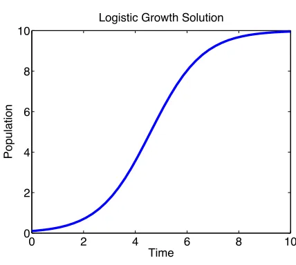
The graph in Figure 1.4 shows the solution to (1.19) with specific parameters. The parameters in this model arer,K, andx0and their impact on the outputx is of interest. Letxr(t) =d xd r,xK(t) =d Kd x, andxx0(t) =
d x
d x0. We can directly calculate the sensitivity equations using (1.14) as a guide to obtain d x
d t =r x(1− x K ), d xr
d t = (r−
2r
K x(t))xr+x(t)−
1
K x 2(t),
d xK d t = (r−
2r
K x(t))xK + r K2x
2(t), d xx0
d t = (r−
2r
K x(t))xx0,
and initial conditions
x(0) =x0, xr(0) =0,
xK(0) =0,
xx0(0) =1.
0 2 4 6 8 10
0 2 4 6 8 10
Logistic Growth Solution
Time
Population
Figure 1.4Solution to (1.19) withK =10,r=1 andx0=.1.
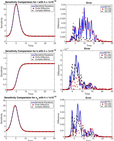
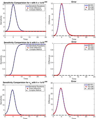
The graphs on the left in Figure 1.5 and Figure 1.6 have the sensitivities using (1.4) and automatic differentiation (blue solid line), central difference (red dotted line), and complex step method (black dashed line). The graphs on the right are the errors between the sensitivity equations (SE) and finite difference (blue solid line), finite difference (FD) and complex step method (red dotted line), and complex step method (CM) and sensitivity equations (black dashed line). It is observed in Figure 1.5 that ath=1×10⁻¹⁰all 3 methods are nearly the same with small error. However, ashgets smaller in Figure 1.6, the central difference method becomes inaccurate, but the complex step method continues to be precise forh=1×10−200. In fact, with machine accuracy 1×10−323, the complex
Time
0 5 10 15 20 25
Sensitivity -2 0 2 4 6 8 10
12Sensitivity Comparision for r with h = 1x10 -10
Sensitivity Equations Finite Difference Complex Method
Time
0 5 10 15 20 25
Difference 0 0.005 0.01 0.015 0.02 0.025 0.03 0.035 0.04 Error SE-FD FD-CM SE-CM Time
0 5 10 15 20 25
Sensitivity 0 0.2 0.4 0.6 0.8 1 1.2
1.4Sensitivity Comparision for k with h = 1x10 -10
Sensitivity Equations Finite Difference Complex Method
Time
0 5 10 15 20 25
Difference #10-4 0 1 2 3 4 5 6 7 8 Error SE-FD FD-CM SE-CM Time
0 5 10 15 20 25
Sensitivity -5 0 5 10 15 20 25 30
Sensitivity Comparision for x
0 with h = 1x10 -10
Sensitivity Equations Finite Difference Complex Method
Time
0 5 10 15 20 25
Difference 0 0.01 0.02 0.03 0.04 0.05 0.06 Error SE-FD FD-CM SE-CM
Time
0 5 10 15 20 25
Sensitivity -2 0 2 4 6 8 10
12Sensitivity Comparision for r with h = 1x10 -200
Sensitivity Equations Finite Difference Complex Method
Time
0 5 10 15 20 25
Difference 0 2 4 6 8 10 12 Error SE-FD FD-CM SE-CM Time
0 5 10 15 20 25
Sensitivity 0 0.2 0.4 0.6 0.8 1
Sensitivity Comparision for k with h = 1x10-200
Sensitivity Equations Finite Difference Complex Method
Time
0 5 10 15 20 25
Difference 0 0.2 0.4 0.6 0.8 1 Error SE-FD FD-CM SE-CM Time
0 5 10 15 20 25
Sensitivity 0 5 10 15 20 25 30
Sensitivity Comparision for x0 with h = 1x10-200
Sensitivity Equations Finite Difference Complex Method
Time
0 5 10 15 20 25
Difference 0 5 10 15 20 25 30 Error SE-FD FD-CM SE-CM
1.3.2 Identifiability Analysis
After deciding which parameters are sensitive, consideration is given to understanding which sensitive parameters can uniquely be identified from the data. The structure of the model as well as amount of data can affect whether a parameter is identifiable. A parameterq is locally identifiable if for an open neighborhood aboutq in the parameter space, y(q1) = y(q2)is true implies that q1=q2[71]. We illustrate how model structure can affect identifiability by considering the parameters aandbwithin the simple ODE:
d x
d t =a b x. (1.21)
We observe thata andb are unidentifiable as there are many possible values fora andb that result in the same producta b.a=2 andb=1 results in the same solution to (1.21) asa=1 and
b=2. Thus, estimating the parameters in this model is futile because of the lack of uniqueness. An identifiability analysis will aid us in deciding which parameters can be uniquely estimated from the experimental data as it is desirable to estimate parameters that are both sensitive and identifiable. Consider the parameters contained inqwhich minimize the cost function
J(q) = 1 N
N
X
i=1
(Vdi−V(ti;q))2,
withV(ti;q)denoting the model output andVdi denoting the corresponding data value at time pointti fori =1, . . .N, whereN is the number of data values. Assume thatq∗is the minimum of this cost function. Then by using a Taylor series expansion aroundq∗, we obtain
V(ti,q) =V(ti;q∗) +
d V(ti;q∗)
d q (q−q
∗) +. . .
If we only consider the first two elements ofV(ti,q)under the assumption thatq≈q∗and substitute this expression into the cost function we find that
J(q) = 1 N
N
X
i=1
Vdi−V(ti;q∗)−d V(ti;q
∗)
d q (q−q
∗)2,
= 1
N
N
X
i=1 d V(t
i;q∗)
d q (q−q
∗)2,
where we used the fact thatq∗is the minimum of the cost function so thatVdi≈V(ti;q∗). Let
S=d V d q =
d V d q1(t1)
d V
d q2(t1) · · ·
d V d ql(t1)
d V d q1(t2)
d V
d q2(t2) · · ·
d V d ql(t2)
..
. ... ... ... d V
d q1(tN)
d V
d q2(tN) · · ·
d V d ql(tN)
, (1.23)
be a(N×l)sensitivity matrix relating to the sensitivitiesd qd V
j(ti)of the output withi=1, . . . ,N and
j=1, . . . ,l, wherel denotes the number of parameters. The cost function of (1.22) is rewritten in terms of this sensitivity matrix
J(q) =1
N(S(q−q
∗))T(S(q
−q∗)), =1
N(S∆q)
T(S∆q),
where∆q=q−q∗. Rearranging∆q=q−q∗, we formulate the cost function in terms ofq∗+∆q:
J(q∗+∆q) = 1 N∆q
TSTS∆q. (1.24)
If we suppose that∆q is an eigenvector ofSTSwithSTS∆q=λ∆q, then we have
J(q∗+∆q) = 1 N∆q
T(λ∆q), = 1
Nλ||∆q|| 2 2.
Algorithm 1.5
1. Create the matrixSTS, compute its eigenvalues, and order them such that
|λ1| ≤ |λ2| ≤ · · · ≤ |λn|.
2. If|λ1|is less than some thresholdε(typically taken to be 10−4), we say that there is a parameter that is unidentifiable.
3. The largest magnitude component of the eigenvector∆q1associated with the eigenvalueλ1
corresponds to the least identifiable parameter. Remove the corresponding column from S and repeat step 1.
1.3.3 Data Analysis
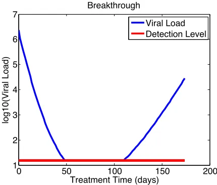
Occasionally, there is data that one cannot observe. For instance in infectious diseases, due to different patient responsiveness to drug treatment, there is viral load data that we are not able to examine with the technology used. Specifically, the exact data measurement is below what is called the lower limit of quantification(LLOQ). This data is considered to be left-censored. Censored data is sometimes excluded in model calibration which can result in inaccurate parameter estimates. The importance of understanding the data below LLOQ can be seen in an example of a Breakthrough patient’s viral load shown in Figure 1.7.
0 50 100 150 200
1 2 3 4 5 6 7
Treatment Time (days)
log10(Viral Load)
Breakthrough
Viral Load Detection Level
The viral load in Breakthrough patients goes below LLOQ (detection level) and rises back up during treatment. This patient behavior will not be accurately modeled without robust predictions for what is occurring beneath the censoring line. Thus, when there is censored data, expectation maximization(EM)[39]is used to compute maximum likelihood estimates for the parameters,
q. A derivation of the EM algorithm that is employed is provided and uses similar notation and techniques as in[7]. Consider the general objective function
q∗=arg minJ(q) = 1 N
N
X
i=1
|ydi−y(ti,q)|2, (1.25)
whereN is the number of data points,ydi is the data at timeti, andy is the model output over an admissible parameter spaceω⊂Rpsuch thatpis the number of parameters being estimated. Since,
in general, the model output, data, and parameters have a large range of values, they are log10scaled. Assume for true parameterq0and varianceσ2that the log scaled data is normally distributed such
that
ydi∼ N(y(ti,q0),σ2).
Letyi=y(ti,q)andL=log(L LOQ). The data can be written as the piecewise function
di=
ydi ifydi>L L ifydi≤L
,
with
Xi=I{yi d>L},
whereI{yi
d>L}is an indicator function such that ify
i
d>LattithenXi=1, otherwiseXi=0. Before presenting the likelihood function to be maximized, standard probability tools are introduced. The standard probability density function(pdf ) for mean 0 and unit variance is given by
ϕ(ξ) =p1
2πe −ξ2
2 ,
which gives the probability that a continuous random variable has the valueξ. The pdf has corre-sponding cumulative distribution function(cdf ),
Φ(ξ) = Z ξ
−∞
which gives the probability of a continuous random variable being less than or equal toξ. Since the censored data is bounded above, it is assumed to follow a truncated normal distribution so that the likelihood function for a sample pointdiis given by
M(q,σ) = N
Y
i=1 1
σϕ di−y
i
σ Xi
Φ di−yi
σ
1−Xi
, (1.26)
where the first term accounts for the probability of observingdi if it is uncensored and the second term accounts for the probability of observingdi if it is censored. Computing log(M)gives the log-likelihood function
M(q,σ) = N
X
i=1
Xilogϕ d i−y
i
σ
−logσ+ 1−XiΦ d
i−y i
σ
. (1.27)
Since in the first term of (1.26),di=ydi, and in the second term,di=L, (1.27) is rewritten as
M(q,σ) = N
X
i=1
Xilogϕ y i d−yi
σ
−logσ+ 1−XiΦ L−yi σ
. (1.28)
EM is used to maximizeM by iteratively improvingqandσuntil the maximum is achieved. A lower truncated normal distribution is considered so the following is true:
E[ydi|ydi≤L] =yi−σΛ(ξi), whereξi=L−yi
σ andΛ(ξi) =ϕ(ξ
i)
Φ(ξi). The following theorem from[50]gives an important result about
truncated normal distributions.
Theorem 1.3.1 If x∼ N [µ,σ2]and a is a constant, then
E[x|truncation] =µ+σλ(α),
V a r[x|truncation] =σ2[1−δ(α)],
whereα=aσ−µsuch that
λ(α) = ϕ(α)
1−Φ(α) if truncation is x >a, λ(α) =ϕ(α)
Hereϕ(α)is the standard normal density withΦ(α)cumulative distribution function, and δ(α) =λ(α)[λ(α)−α].
Theorem 1.3.1 along with the relationship between the expected value,E(X), and the variance,
V a r(X),
V a r(X) =E(X2)−E2(X), =⇒ E(X2) =V a r(X) +E2(X),
gives the following
E[(ydi)2|ydi≤L] =V a r[ydi|ydi≤L] +E2[ydi|ydi≤L], =σ2(1
−Λ(ξi)[Λ(ξi)−ξi]) + (yi−σΛ(ξi))2, =σ2−σ2Λ(ξi)2+σ2Λ(ξi)ξi+y2
i −2σΛ(ξ i)y
i+σ2Λ(ξi)2, =yi2−2σΛ(ξi)yi−σ2ξiΛ(ξi) +σ2.
The censored data is updated with
¯
yi=Xiydi+ (1−Xi)E[ydi|ydi≤L], =Xiydi+ (1−Xi)[yi−σΛ(ξi)]. The squared residuals are updated through
¯
ri=XiE[(ydi−yi)2] + (1−Xi)E[(ydi−yi)2|ydi≤L]. =Xi(ydi−yi)2+ (1−Xi)[E[(ydi)
2
|ydi≤L]−2yiE[ydi|y i
d≤L] +y
2
i ], =Xi(ydi−yi)2+ (1−Xi)σ2[1−ξiΛ(ξi)].
The EM Algorithm is presented in algorithm (1.6). A stopping criterion for this algorithm is the relative change between ˆq, ˆσ. EM results in estimates of the expected value and variance for the censored data.
1.3.4 Confidence and Prediction Intervals
Algorithm 1.6
1. Estimate ˆq0usingyd and ordinary least squares where the censored data is adjusted by half to L2. Setk=0 and compute an initial estimate forσ2from
(σˆ(0))2= 1
N
N
X
i=1
|y¯i−y(ti; ˆq(0))|2.
2. Let ˆyi(k)=y(ti, ˆq(k))and ˆξi(k)= L−yi(k)
ˆ
σ(k) and update the data and residuals by
¯
yi(k)=Xiydi+ (1−Xi)[yˆi(k)−σˆ(k)Λ(ξˆi(k))], ¯
ri(k)=Xi(ydi−yˆi(k))2+ (1−Xi)(σˆ(k))2[1−ξˆi(k)Λ(ξˆi(k))]. 3. Compute ˆq(k+1), ˆσ(k+1)using ordinary least squares by solving
ˆ
q(k+1)=arg min 1
N
N
X
i=1
|y¯i(k)−y(ti,q)|2,
and updating ˆσwith
(σˆ(k+1))2= 1
N
N
X
i=1
¯
parameters. In calculating these intervals, standard errors are computed from the model predictions using the parameters that have been estimated. Techniques and notation as in[5, 7, 13, 88, 94]are used.
1.3.4.1 Parameter Confidence Intervals
Consider the statistical model
Yj ≡f(tj,q~0) +εj, j=1, 2, ...,N, (1.29)
forN observations wheref is the model in terms of the theoretical true parameter values,q~0∈Rp.
The errors,εj, are assumed to be independent and identically distributed (i.i.d.) random variables with meanE[εj] =0 and variance,V a r(εj) =σ20whereσ02is unknown. Thus,Yj are i.i.d. with meanf(tj,q~0)and varianceσ20. The parameters,q, are estimated using the ordinary least squares
approach
q∗=arg minJ(q) =
N
X
j=1
|yj−f(ti,q~)|2, (1.30)
where{yj}is a realization of the observation process{Yj}andq∗is an estimator that depends on the sampling size. SinceYj is a random variable, so isq∗with a distribution called the sampling distribution. A sampling distribution characterizes the distribution of all the values an estimator{q∗}
could have across all realizations{yj}with data size,N, that could be collected. Thus, the standard errors provide a measure of the extent of uncertainty involved in estimatingqusing the estimator
q∗with sample sizeN. Herep-multivariate Gaussian distributions with asymptotic convergence in distribution, meanE[q∗(Y~)] ≈q~
0, and covariance matrixΣ0 ≈σ20(ST(q0)S(q0))−1 are used to
approximate the sampling distribution. Asymptotic convergence in distribution means that the cumulative distribution functions converge asN → ∞. HereS(q0)is the sensitivity matrix similar
to (1.23). Consequently, the sampling distribution approximates satisfy
q∗(Y)∼ Np(q0,Σ0)≈ Np(q0,σ02(S
T(q
0)S(q0))−1), (1.31)
for largeN. Note thatσ20is approximated by
σ2 0≈σˆ
2= 1
N−p
N
X
j=1
The standard errors that will be used in the half-widths of the confidence intervals are given by
S Ek(q) =
Æ
Σk k(q),k =1, 2, ...,p. Thus, a 100(1−α)% confidence interval for parameterqk is
ˆ
qk±τN1−−αp 2
ˆ
σkS Ek(q)
whereτN1−−αp
2 is the 1−
α
2 quantile of a student’st-distribution withN−pdegrees of freedom.α=.05
since 95% confidence intervals are used.[49, 88]Given the parameter estimates, the next step is quantifying the accuracy in the model predictions.
1.3.4.2 Predictive Confidence Intervals
An understanding of the uncertainty in the model predictions is important for making conclusions. This is determined by calculating predictive confidence intervals. Consider an estimation of the true mean response, ¯yj, of the output
ˆ
yj =f(tj, ˆq),
where ˆqis an estimate of the solution to (1.30). Note that ˆq is close to the true value,q0, for largeN
so
∇f(tj,q0)≈ ∇f(tj, ˆq).
This implies that
E[yˆj] =y¯j,
and by using Taylor series, the following is observed
V a r[yˆj] =V a r[f(tj, ˆq)],
≈V a r[f(tj,q0) +∇f(tj,q0)(qˆ−q0)], =V a r[f(tj,q0)] +V a r[∇f(tj,q0)(qˆ−q0)],
=∇f(tj,q0)TV a r[(qˆ−q0)]∇f(tj,q0),
=σ2
0∇f(tj,q0)T(S(q0)TS(q0))−1∇f(tj,q0).
Thus,
ˆ
yj−y¯j ˆ
σpv0 ∼τ
N−p
![Figure 1.1 A simplex and points considered during the Nelder-Mead algorithm from [37].](https://thumb-us.123doks.com/thumbv2/123dok_us/1624527.1202142/23.612.227.403.103.258/figure-simplex-points-considered-nelder-mead-algorithm.webp)
![Table 3.1 Typical values from [95].](https://thumb-us.123doks.com/thumbv2/123dok_us/1624527.1202142/63.612.232.399.103.309/table-typical-values-from.webp)
![Figure 3.1 Simulation of (3.5) with initial conditions [T0,I0,VI 0] = [1.92 × 107,0,1].](https://thumb-us.123doks.com/thumbv2/123dok_us/1624527.1202142/68.612.210.421.593.640/figure-simulation-initial-conditions-t-i-vi.webp)
