Statistical Modeling for Population

(1)

ISSN(Online): 2319-8753 ISSN (Print): 2347-6710

I

nternational

J

ournal of

I

nnovative

R

esearch in

S

cience,

E

ngineering and

T

echnology

(A High Impact Factor & UGC Approved Journal)

Website: www.ijirset.com

Vol. 6, Issue 9, September 2017

Statistical Modeling for Population

M.Rajani1, Sk. Hussain Saheb2, S. Damodharan3, Dr. K. Murali4, Dr.M.Subbarayudu5

Research Scholar, Department of Statistics, S.V. University, Tirupati, AP, India1, 2, 3

Academic Consultant, Department of Statistics, S. V. University, Tirupati, AP, India4

Professor & Chairman BOS, Department of Statistics, S.V. University, Tirupati, AP, India5

ABSTRACT: A best linear statistical model for total population is selected using stepwise regression with the available independent variables namely number of births, number of deaths, per capita income and total population with one time lag period related to the data of India, Andhra Pradesh, Tamil Nadu, Kerala and Karnataka during 2000-2015. Chow test and dummy variable technique is applied for testing the structural change (shift) within India, Andhra Pradesh, Tamil Nadu, Kerala and Karnataka in two selected period 2000-2007 and 2008-2015, also between the four states Andhra Pradesh, Tamil Nadu, Kerala and Karnataka during 2000-2015.Through numerical analysis it is observed that there is no any shift in total population within India, Andhra Pradesh, Tamil Nadu and Kerala in the two periods 2000-2007 and 2008-2015 but there is shift in Karnataka. Also there is no structural change between the four southern states of India during 2000-2015.

KEY WORDS: Linear statistical model, Inference in linear model, Stepwise regression, Chow test, Dummy variable technique.

I. INTRODUCTION

The purpose of the present study is to construct chow test for structural change in ‘total population’ and also to develop dummy variable technique for the same assuming a linear relationship between the dependent variable ‘total population’ (Yt) and four independent variables namely number of births (NB), number of deaths (ND), per capita

income (PCI) and total population with one time lag period (Yt-1) using stepwise regression for testing the structural

change. Empirical study is conducted for the data of India, Andhra Pradesh, Tamil Nadu, Kerala and Karnataka individually for structural change between the two periods 2000-2007 and 2008-2015, also among the four states Andhra Pradesh, Tamil Nadu, Kerala and Karnataka during 2000-2015. Relevant data is collected from Directorate of Economics and Statistics, Central Statistics Office, Annual Reports on the Registration of Births and Vital Statistics of India Based on the Civil Registration System.

II. METHODOLOGY

To study the structural change in total population between the two periods 2000-2007 and 2008-2015 for India, Andhra Pradesh, Tamil Nadu, Kerala and Karnataka independently, we have to select a best linear relationship between the dependent variable total population and the four independent variables number of births, number of deaths, per capita income and total population with one time lag period through stepwise regression for the study period 2000-2015. After selecting the best regression model, we construct chow test and dummy variable approach for testing the structural change between the two time periods 2000-2007 and 2008-2015.

And for testing the structural change among the four southern states of India namely Andhra Pradesh, Tamil Nadu, Kerala and Karnataka during the time period 2000-2015, we proceed as follows

(i) Arrange the data of four states on dependent and four independent variables one below the other.

(2)

I

nternational

J

ournal of

I

nnovative

R

esearch in

S

cience,

E

ngineering and

T

echnology

(iii) Use the above selected model for testing the structural change in total population through chow test and dummy variable approach.

STEPWISE REGRESSION:

1. Fit the regression model with all available independent variables.

2. Compute t-calculated values corresponding to regression coefficients of each independent variable of the model. 3. Omit the independent variables from the regression model whose calculated t-values are less than one.

4. Refit the regression model with independent variables whose t-calculated values are greater than one. 5. Again calculate the t-values for the regression coefficients of independent variables which are in the model. 6. Finally we select the model with independent variables whose t-calculated values are greater than one.

This procedure is called stepwise regression.

CHOW TEST:

To study the structural change between two sets of observations in the linear relationship between a dependent variable Y and a set of two independent variables X1and X 2 we make use of chow test which is developed by G.C.Chow(1960).

Let n1 be the number of observations on the variables. Suppose, further we obtain additional n2 observations on the

same variables. Denote n1, n2 as the number of observations in first and second sets of data respectively.

Let the relation between Y and X1, X 2 be

= + + + (1)

In particular this relation for the two sets namely first and second of data may be written respectively as

= + + + , = 1, 2, … , (2) = + + + , = 1, 2, … , (3)

In equations (2) and (3) ε’s are stochastic error terms. It is assumed that ε2 has the same normal distribution

as ε1 with variance covariance matrix σ2I . Y1 ,Y2 are first and second sets of observations respectively on dependent

variable Y.

Given (2) and (3) we can think of the following possibilities regarding the coefficients.

i. α1 = α2 ; β1= β2 ; γ1 = γ2 (4a)

i.e., all the coefficients are same in the two regressions.

ii. α1≠ α2 ; β1= β2 ; γ1 = γ2 (4b)

i.e., the two regressions are different in intercepts only.

iii. α1 = α2 ; β1 ≠ β2 ; γ1 = γ2 (4c)

i.e., the two regressions are different in X1 coefficients only.

iv. α1≠ α2 ; β1 ≠ β2 ; γ1 ≠ γ2 (4d)

i.e., the two regressions are different in all regression coefficients.

In the similar fashion we may have different possibilities. To test whether the two regressions are different or not we can construct the Chow test procedure as follows

i. Combine all the (n1+n2) observations and compute the OLS estimates of α, β and γ, from the combined

regression equation (1). From this obtain the residual sum of squares S1 with degrees of freedom (n1+n2-k), k

(3)

I

nternational

J

ournal of

I

nnovative

R

esearch in

S

cience,

E

ngineering and

T

echnology

ii. Run the regressions (2) and (3) separately and obtain the respective residual sum of squares say S2 and S3 with

degrees of freedom n1-k and n2-k respectively. Add these two residual sum of squares and denote it as S4.

i.e., S4 = S2 + S3 with degrees of freedom (n1+n2 -2k)

iii. Obtain S5 = S1 – S4 with degrees of freedom k.

iv. Apply the F-test

= ⁄

( )

⁄ ~ ( , ) (5)

If F-calculated value is greater than F-critical value, reject the hypothesis that the parameters α’s, β’s and γ’s are the same for two sets of observations, otherwise accept the hypothesis at required level of significance.

This procedure may be extended to any number of independent variables and any number of sets of observations. Chow test is general in nature, it merely tells whether the regressions are different or not without specifying whether the differences if any is due to difference in intercept terms or due to difference in the coefficients of particular explanatory variables.

DUMMY VARIABLE APPROACH:

Dummy variable approach for structural change is developed by Damodar Gujarati (1970).To test the structural change between the two sets of data namely (2) and (3), we consider the following equation

= + + + + + + , i =1, 2, 3, ….. (n1+n2) (6)

Here

D = 1, if the observation belongs to set-2 = 0, other wise

a0 : Intercept for set-1

a1 : Differential intercept for set-2.

a2, a4 : Slope co-efficient of Y with respect to X1and X2respectively for set-1.

a3, a5 : Differential slope co-efficient of Y with respect to X1and X2 respectively for set-2.

From the above differential intercepts and differential slope coefficients we can easily obtain the actual values of intercept and slope coefficients for two sets as follows.

For set-1: Y1 = a0 + a2 x1 + a4 x2 (7)

For set-2: Y2= (a0+a1) + (a2+a3) x1 + (a4+a5) x2 (8)

To determine the equations (7) and (8), we need equation (6) which can be estimated by the method of ordinary least squares.

Depending up on the statistical significance of estimated differential intercepts and differential slope coefficients one can find out whether the sets of linear regression coefficients are different or not. This procedure may be extended to any number of independent variables and any number of sets of observations.

III. EMPIRICAL STUDY FOR STRUCTURAL CHANGE

(4)

I

nternational

J

ournal of

I

nnovative

R

esearch in

S

cience,

E

ngineering and

T

echnology

CHOW TEST FOR TWO PERIODS 2000-2007 AND 2000-2015:

For India, the best regression model using stepwise regression is

Yt = 5341.6677 + 0.0001 NB+ 0.0056 PCI+ 0.3289 Yt-1 (9)

S1= 150142.1856, S2= 75467.9878, S3= 9.0209

S4= 75477.0087, S5=74665.1768, F = 1.9785

Since F(4,8) at 5% = 3.838, we accept H0 and conclude that there is no structural change in the two periods.

For Andhra Pradesh, the best regression model using stepwise regression is

Yt = 70.1738 + 0.0002 NB + 0.5729 Yt-1 (10)

S1= 106837.5884, S2= 25.7325, S3= 91469.2162

S4= 91494.9486, S5=15342.6398, F =0.5590

Since F(3,10)at 5% = 3.7083, we accept H0 and conclude that there is no structural change in the two periods.

For Tamil Nadu, the best regression model using stepwise regression is

Yt = 80.3169 + 0.0003 NB+ 0.0007 ND (11)

S1= 1334.684378, S2= 607.2732, S3= 287.4006

S4= 894.6738, S5=440.0105, F =1.6394

F(3,10)at 5% = 3.7083, we accept H0 and conclude that there is no structural change in the two periods.

For Kerala, the best regression model using stepwise regression is

Yt = 105.5237 + 0.0001 ND+ 0.6289 Yt-1 (12)

S1= 133.2525, S2= 0.6726, S3= 96.1057

S4= 96.7783, S5= 36.4743, F = 1.2563

For Karnataka, the best regression model using stepwise regression is

Yt = 107.4183 + 0.0003 PCI+ 0.8031 Yt-1 (13)

S1= 247.5822, S2= 36.6048, S3= 95.1998

S4= 131.8047, S5=115.7775, F =2.9280

Since F(3,10) at 10% = 2.728, we reject H0 and conclude that there is structural change in the two periods.

CHOW TEST FOR FOUR STATES ANDHRA PRADESH, TAMIL NADU, KERALA AND KARNATAKA:

The best regression model using the data of four states (64 observations) through stepwise regression is Yt = -10.4862 + 0.0003 ND+ 0.8450 Yt-1 (14)

S1= 122631.4065, S2= 106837.5884, S3= 1334.684378, S4= 133.2525

S5=247.5822, S6= 108553.1075, S7= 1564.25544, F = 0.7493

DUMMY VARIABLE APPROACH FOR TWO PERIODS 2000-2007 AND 2008-2015:

For India, the model can be written as

0 1 2 3 4 5 6 1 7 1

t t t t

Y



a



a D a B



a DNB



a PCI



a DPCI



a Y

_



a DY

_





(5)

I

nternational

J

ournal of

I

nnovative

R

esearch in

S

cience,

E

ngineering and

T

echnology

Table (1): India-Estimation of parameters

Variables Parameters Coefficients Standard Error t Stat P-value

Intercept a0 1077.7566 2273.1642 0.4741 0.6481

D a1 -754.8892 11245.9341 -0.0671 0.9481

NB a2 0.0003 0.0001 4.3965 0.0023

DNB a3 -0.0003 0.0002 -1.3081 0.2272

PCI a4 -0.0877 0.0431 -2.0338 0.0764

DPCI a5 0.0877 0.0471 1.8625 0.0995

Yt-1 a6 0.7004 0.2343 2.9886 0.0174

D Yt-1 a7 0.2883 1.2816 0.2250 0.8277

For Andhra Pradesh, the model can be written as

0 1 2 3 4 1 5 1

t t t t

Y



a



a D a NB



a DNB



a Y

_



a DY

_





(16)

Table (2): Andhra Pradesh - Estimation of parameters

Intercept a0 -7.8728 1737.2255 -0.0045 0.9965

D a1 -45.6681 1758.0333 -0.0260 0.9798

NB a2 0.0000 0.0005 0.0042 0.9968

DNB a3 0.0003 0.0006 0.6018 0.5607

Yt-1 a4 1.0179 2.6931 0.3780 0.7134

D Yt-1 a5 -0.4391 2.7103 -0.1620 0.8745

For Tamil Nadu, the model can be written as

0 1 2 3 4 5

t t

Y



a



a D a NB



a DNB



a ND



a DND





(17)

Table (3) : Tamil Nadu -Estimation of parameters

Intercept a0 161.8998 533.9083 0.3032 0.7679

D a1 -56.0622 537.5380 -0.1043 0.9190

NB a2 0.0002 0.0004 0.5310 0.6070

DNB a3 0.0001 0.0004 0.2947 0.7743

ND a4 0.0006 0.0003 2.1339 0.0586

DND a5 -0.0001 0.0003 -0.4200 0.6833

For Kerala, the model can be written as

0 1 2 3 4 1 5 1

t t t t

Y



a



a D a ND



a DND



a Y

_



a DY

_





(6)

I

nternational

J

ournal of

I

nnovative

R

esearch in

S

cience,

E

ngineering and

T

echnology

Intercept a0 -21.7689 157.6890 -0.1380 0.8929

D a1 298.9755 191.4328 1.5618 0.1494

NB a2 0.0000 0.0002 -0.1312 0.8982

DNB a3 0.0000 0.0002 -0.0198 0.9846

Yt-1 a4 1.0916 0.6029 1.8105 0.1003

D Yt-1 a5 -0.8833 0.6719 -1.3146 0.2180

For Karnataka, the model can be written as

0 1 2 3 4 1 5 1

t t t t

Y



a



a D



a PCI



a DPCI



a Y

_



a DY

_





(19)

Table (5): Karnataka -Estimation of parameters

Intercept a0 -5.5355 81.0854 -0.0683 0.9469

D a1 570.1767 207.0931 2.7532 0.0204

PCI a2 -0.0002 0.0005 -0.4401 0.6692

D PCI a3 0.0013 0.0006 2.2973 0.0445

Yt-1 a4 1.0333 0.1673 6.1777 0.0001

DYt-1 a5 -1.0811 0.3894 -2.7763 0.0196

Regarding India, Andhra Pradesh, Tamil Nadu, Kerala from tables (1), (2), (3) and (4) respectively, we observed that none of the differential intercepts and differential slope coefficients are significant at 5% level of significance. Hence we infer that there is no structural change in total population between the two time periods 2000-2007 and 2008-2015.

Regarding Karnataka from table (5), it is observed that the differential intercept a1 and differential slope

coefficients a3, a5 are significant at 10 % level, hence we infer that there is structural change in total population during

2008-2015 with respect to the per capita income (PCI) and total population with one time lag period (Yt-1).

DUMMY VARIABLE APPROACH FOR FOUR STATES ANDHRA PRADESH, TAMIL NADU, KERALA AND KARNATAKA:

To test the structural change in total population in four selected states Andhra Pradesh, Tamil Nadu, Kerala and Karnataka during the period 2000-2015, the model can be written as

=

+ + + + + + + + + + +

+ , i =1, 2, 3, ….. (n1+n2 +n3+n4) (20)

Where

Yt = Total population

ND = Number of deaths

Yt-1 = Total population with one time lag period D1 = 1, if the data belongs to Tamil Nadu State

(7)

I

nternational

J

ournal of

I

nnovative

R

esearch in

S

cience,

E

ngineering and

T

echnology

D2 = 1, if the data belongs to Kerala State

= 0, otherwise

D3 = 1, if the data belongs to Karnataka State

= 0, otherwise

Also ai’s entering into (20) are interpreted as follows:

a0 : Intercept for the model of Andhra Pradesh.

a1, a2, a3 : Differential intercept for the models of Tamil Nadu, Kerala and Karnataka respectively.

a4, a8 : Slope co-efficient of Yt with respect to ND, Yt-1 respectively for the state Andhra Pradesh.

a5, a9 : Differential slope co-efficient of Yt with respect to ND, Yt-1 respectively for the state Tamil Nadu.

a6, a10 : Differential slope co-efficient of Yt with respect to ND, Yt-1 respectively for the state Kerala.

a7, a11 : Differential slope co-efficient of Yt with respect to ND, Yt-1 respectively for the state Karnataka.

From the above differential intercepts and differential slope coefficients we can easily obtain the actual values of intercept and slope coefficients for four states as follows.

For Andhra Pradesh state

Y1 = a0 + a4ND + a8 Yt-1 (10)

For Tamil Nadu state

Y2 = (a0+a1) + (a4+a5) ND + (a8+a9) Yt-1 (11)

For Kerala state

Y3 = (a0+a2) + (a4+a6) ND + (a8+a10) Yt-1 (12)

For Karnataka state

Y4 = (a0+a3) + (a4+a7) ND + (a8+a11) Yt-1 (13)

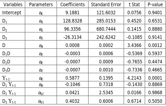
Table (6) : Estimation of parameters

Intercept a0 9.1881 121.6032 0.0756 0.9401

D1 a1 128.8328 285.0153 0.4520 0.6531

D2 a2 96.3356 680.7444 0.1415 0.8880

D3 a3 -26.3134 242.6242 -0.1085 0.9141

D a4 0.0008 0.0002 3.4366 0.0012

D1D a5 -0.0003 0.0006 -0.5369 0.5937

D2D a6 -0.0007 0.0009 -0.7655 0.4474

D3D a7 -0.0007 0.0010 -0.7336 0.4665

Yt-1 a8 0.5877 0.1395 4.2143 0.0001

D1 Yt-1 a9 -0.1046 0.7318 -0.1430 0.8869

D2 Yt-1 a10 0.0421 2.5345 0.0166 0.9868

D3 Yt-1 a11 0.4032 0.6006 0.6714 0.5050

(8)

I

nternational

J

ournal of

I

nnovative

R

esearch in

S

cience,

E

ngineering and

T

echnology

IV. CONCLUSIONS

In the present study a best linear relationship is established using stepwise regression between the dependent variable total population and four independent variables namely number of births, number of deaths, per capita income and total population with one time lag period relating to the data of India, Andhra Pradesh, Kerala and Karnataka independently during the period 2000-2015. Also combining the data of four states a best linear relationship is found out using stepwise regression. Later we applied chow test for testing the shift in total population between the two periods 2000-2007 and 2008-2015 using the corresponding best linear regression within India, Andhra Pradesh, Kerala and Karnataka. Also the same test is applied for testing the shift in total population between the four southern states of India during the period 2000-2015.

Dummy variable approach for testing the shift in total population within India, Andhra Pradesh, Kerala and Karnataka is conducted independently also tested the shift in total population between the four southern states of India.

Using chow test and dummy variable approach it is concluded that there is no shift in the total population within India, Andhra Pradesh, Tamil Nadu and Kerala between the two periods 2000-2007 and 2008-2015, there is no shift in the population between the southern states India during 2000-2015. But using chow test it is observed that there is shift in the total population in Karnataka state between the two periods 2000-2007 and 2008-2015. In particular using dummy variable approach it is observed that there is shift in the period 2008-2015 with respect to intercept per capita income and total population with one time lag period.

APPENDIX

INDIA

year

Population (Lakhs)

No of Births

No of

Deaths PCI Yt-1

2000 10534.81 12946823 3789466 15881 10349.77

2001 10287.37 12993577 3961767 16688 10534.81

2002 10901.89 15645632 4436100 17782 10287.37

2003 11083.70 15290261 4569026 18885 10901.89

2004 11264.19 15777612 4487886 20871 11083.70

2005 11443.26 16394625 4602727 23198 11264.19

2006 11620.88 18121296 5298279 26003 11443.26

2007 11796.86 19469756 5804922 29524 11620.88

2008 11970.70 19993799 5638131 33283 11796.86

2009 12141.82 21292574 5677705 37490 11970.70

2010 12309.84 21430434 5690549 46117 12141.82

2011 12474.46 21836920 5735082 53331 12309.84

2012 12635.90 21951519 5850176 67839 12474.46

2013 12794.99 22482951 6086616 68757 12635.90

2014 12952.92 23001523 6138182 74920 12794.99

(9)

I

nternational

J

ournal of

I

nnovative

R

esearch in

S

cience,

E

ngineering and

T

echnology

ANDHRA PRADESH TAMIL NADU

year

Population (Lakhs)

No of

Births No of Deaths PCI Yt-1

Population (Lakhs)

No of Births

No of

Deaths PCI Yt-1

2000 760.45 933717 350909 15427 754.27 616.00 1114828 356257 18367 626.29

2001 765.42 881256 359615 17195 760.45 621.83 1101376 387451 20367 616.00

2002 777.10 986599 369331 18573 765.42 627.42 1107351 403422 21239 621.83

2003 786.16 913607 374679 19434 777.10 663.32 1088659 420107 21738 627.42

2004 795.02 952629 375521 21931 786.16 638.83 1091016 408799 24087 663.32

2005 803.69 933498 354261 23925 795.02 644.16 1071863 419119 27512 638.83

2006 812.19 1124280 403800 26662 803.69 644.16 1054929 443503 31663 644.16

2007 820.49 1184555 427698 30439 812.19 654.35 1073635 433970 37190 644.16

2008 828.58 1179114 412561 35600 820.49 659.19 1053826 429981 40757 654.35

2009 836.49 1164942 434064 40902 828.58 663.86 1058142 447900 45058 659.19

2010 841.29 1192721 415050 52814 836.49 676.32 1065271 472450 63547 663.86

2011 846.66 1186895 420646 62912 841.29 721.39 1157979 476709 72993 676.32

2012 857.44 1122879 405909 71540 846.66 732.21 1205092 496876 84058 721.39

2013 864.76 722843 248110 72301 857.44 743.19 1185397 507578 98628 732.21

2014 493.87 848883 306618 81397 864.76 754.79 1206850 547579 112664 743.19

2015 513.40 851499 310340 90517 493.87 766.56 1167506 568271 128366 754.79

KERALA KARNATAKA

year

Population (Lakhs)

No of Births

No of

Deaths PCI Yt-1

Population (Lakhs)

No of Births

No of

Deaths PCI Yt-1

2000 317.57 593724 178795 18117 315.3 525.22 1009716 351736 17502 518.18

2001 319.72 579063 182059 20107 317.57 533.21 1017224 365181 18344 525.22

2002 323.03 572847 184597 20287 319.72 539.69 973653 355662 18547 533.21

2003 325.91 549719 194264 22776 323.03 553.27 1001749 359661 19621 539.69

2004 328.75 558933 199017 24492 325.91 559.92 988520 343644 20901 553.27

2005 331.54 555122 204157 27048 328.75 566.47 1007868 364415 26882 559.92

2006 334.26 556326 219094 36276 331.54 572.92 1046531 387604 31239 566.47

2007 336.94 545154 238691 40419 334.26 579.27 1046424 381890 35981 572.92

2008 339.58 535738 221769 45700 336.94 585.52 1082450 372062 42419 579.27

2009 342.16 544348 232020 53046 339.58 591.70 1076383 373290 48084 585.52

2010 344.67 546964 238864 60264 342.16 597.80 1071518 381743 51364 591.70

(10)

I

nternational

J

ournal of

I

nnovative

R

esearch in

S

cience,

E

ngineering and

T

echnology

REFERENCES

[1] Gujarati, Damodar N.(1970a) : Use of Dummy Variables in Testing for Equality between Sets of Coefficients in Two Linear Regressions: A Note”, American Statistician, 24(1):50-52.

[2] Gujarati, Damodar N.(1970b) : Use of Dummy Variables in Testing for Equality between Sets of Coefficients in Two Linear Regressions: A Generalization”, American Statistician, 24(5):18-22.

[3] Chow, G.C. (1960): “Tests of equality between sets of coefficients in two linear regressions”, Econometrica, 28,591-605. [4] Gregory C. Chow. (1983): “Econometrics”, International Edition, McGraw Hill Book Company, SINGAPORE. [5] Norman R. Draper and Harry Smith: Applied regression analysis, Third Edition, Wiley India Pvt. Ltd.

2012 335.52 544388 237615 83725 347.08 609.75 1124490 407015 68053 603.82

2013 337.15 536352 260195 91567 335.52 615.60 1068671 413635 77168 609.75

2014 338.79 534458 248242 103820 337.15 640.55 1087530 411533 89545 615.60