ABSTRACT
JONG, WUCHIEH JAMES. Multicast Access Protocols in an Optical Burst Switched WDM Ring Network. (Under the direction of Professor Harry G. Perros.)
Optical metropolitan area networks are commonly implemented in a ring architecture. In this research, we study various access protocols for multicasting in an optical burst switched (OBS) WDM ring environment. To our knowledge, this is the first detailed study of multicast protocols in an OBS ring architecture. A ring topology is appropriate for multicasting since routing is significantly simplified as compared to a mesh topology. This allows us to forgo complex routing algorithms and focus on performance of various access protocols. We have developed multicast access
protocols that use simple scheduling and coordination schemes, and therefore are easy to implement in hardware. We consider only distributed protocols to avoid having a single point of failure. We study reliable versus unreliable protocols, and collision versus collision-free protocols. Ring nodes are equipped with a single fixed
transmitter and tunable receiver (FT-TR). Signaling is done via a dedicated control wavelength. The performance of the multicast access protocols is analyzed by simulation. We measure the performance of the access protocols in terms of throughput, delay, channel utilization, and fairness. We show that there is a relationship between throughput, delay, and channel utilization. Specifically,
MULTICAST ACCESS PROTOCOLS IN AN OPTICAL
BURST SWITCHED WDM RING NETWORK
by
WUCHIEH JAMES JONG
A thesis submitted to the Graduate Faculty of North Carolina State University
in partial fulfillment of the requirements for the Degree of
Master of Science
COMPUTER SCIENCE
Raleigh 2002
APPROVED BY:
_______________________________ _______________________________
Dedicated to my loving family who made this possible: to my parents, John and Sue, for molding me into who I am, to my siblings, Wuchen and Katherine, for all their encouragements,
BIOGRAPHY
ACKNOWLEDGEMENTS
I would like express my deepest gratitude to my advisor, Dr. Harry Perros, for his guidance in my research thesis. He deserves so much credit for making this a
rewarding, interesting, and challenging learning process. I appreciate all his efforts in supporting my thesis work. I feel honored and privileged to have worked with him.
I would like to thank Dr. George Rouskas and Dr. Douglas Reeves for their advice, professionalism, and service as my committee members. I would like to thank Dr. Carla Savage for her advice and encouragement throughout my graduate studies.
I wish to thank Lisong Xu for his patience in helping me with the simulation. I would like to thank Julie Starr for her cheerful support on the Unix related issues.
Table of Contents
List of Tables...ix
List of Figures ...x
Introduction ...1
1.1 Optical Networks...1
1.2 Wavelength Division Multiplexing ...2
1.3 Motivation ...3
Background and Related Work ...5
2.1 Multicast Communication ...5
2.2 Multicast Support at the WDM Layer ...6
2.3 Topologies for Multicasting ...7
2.3.1 Mesh Networks...7
2.3.2 Ring Networks...8
2.3.3 Broadcast-and-Select Networks ...9
2.4 Related Work...10
2.4.1 Multicasting in Broadcast-and-Select Networks ...10
2.5 Ring and Broadcast-and-Select Networks Comparison ...13
Optical Burst Switching ...14
3.1 Circuit Switching...14
3.2 Packet Switching ...15
3.3 Optical Burst Switching ...16
3.3.1 Control Message...16
3.3.2 Offset ...17
3.3.3 OBS Schemes ...17
System Model ...21
4.1 Ring Architecture ...21
4.2 Node Architecture ...23
4.3 Control Wavelength Operation...25
4.3.1 Control Wavelength and Control Frame Structure...25
4.3.2 Sending and Receiving Burst Information ...25
4.3.3 Control Processing Delay ...26
Multicast Access Protocols...27
5.1 Design Choices...27
5.1.1 Algorithm Complexity...27
5.1.2 Fairness...28
5.1.3 Distributed versus Centralized ...28
5.1.6 Transceiver Tunability...30
5.1.7 Synchronization and Fixed Sized Slots ...30
5.2 Collision Resolution ...31
5.3 Assumptions ...32
5.4 Access Protocols...33
5.4.1 Unreliable ...33
5.4.2 Persistent...35
5.4.3 Unicast Token...37
5.4.4 Multicast Token...40
Numerical Results...43
6.1 Simulation Parameters...43
6.2 Multicast Group Generation ...44
6.3 Traffic Generation ...45
6.4 Simulation Results...46
6.4.1 Effect of Average Arrival Rate...47
6.4.2 Tradeoff between Channel Utilization and Throughput/Delay ...57
6.4.3 Effect of Minimum and Maximum Burst Size ...60
6.4.4 Effect of Number of Multicast Groups...64
6.4.5 Hot Spots ...66
6.5 Summary of Results ...68
Conclusions and Future Research ...70
7.2 Future Research ...71
List of Tables
List of Figures
Figure 1.1: Wavelength Division Multiplexing (WDM)...3
Figure 2.1: Broadcast-and-Select WDM Network (FT-TR) ...9
Figure 3.1: JET Offset ...20
Figure 4.1: Architecture of OBS Ring with N Nodes ...22
Figure 4.2: Architecture of an OBS Node ...22
Figure 6.1: IPP State Transition Model...45
Figure 6.2: Receiver Throughput for N = 10 nodes, G = 9 groups (Uniform)...48
Figure 6.3: Overall Packet Delay for N = 10 nodes, G = 9 groups (Uniform)...51
Figure 6.4: Packet Buffer Loss for N = 10 nodes, G = 9 groups (Uniform) ...51
Figure 6.5: Channel Utilization for N = 10 nodes, G = 9 groups (Uniform) ...53
Figure 6.6: Persistent Retransmissions for N = 10 nodes, G = 9 groups (Uniform) ...53
Figure 6.7: Throughput Fairness Index for N = 10 nodes, G = 9 groups (Uniform)...56
Figure 6.8: Normalized Receiver Throughput from Node 1 to All Other Nodes (Uniform)...56
Figure 6.9: Delay Fairness Index for N = 10 nodes, G = 9 groups (Uniform) ...57
Figure 6.11: Overall Packet Delay for varying TokensNeeded
(Modified Multicast Token) ...59
Figure 6.12: Channel Utilization for varying TokensNeeded (Modified Multicast Token) ...59
Figure 6.13: Receiver Throughput for varying Minimum Burst Size ...60
Figure 6.14: Overall Packet Delay for varying Minimum Burst Size...61
Figure 6.15: Channel Utilization for varying Minimum Burst Size...61
Figure 6.16: Receiver Throughput for varying Maximum Burst Size ...62
Figure 6.17: Overall Packet Delay for varying Maximum Burst Size ...63
Figure 6.18: Channel Utilization for varying Maximum Burst Size ...63
Figure 6.19: Receiver Throughput for varying Multicast Groups...64
Figure 6.20: Overall Packet Delay for varying Multicast Groups...65
Figure 6.21: Channel Utilization for varying Multicast Groups ...65
Figure 6.22: Receiver Throughput for N = 10 nodes, G = 9 groups (Hot Spot) ...67
Figure 6.23: Overall Packet Delay for N = 10 nodes, G = 9 groups (Hot Spot) ...67
Chapter 1
Introduction
1.1 Optical
Networks
During the past decade, the Internet and World Wide Web have experienced tremendous growth in the number of users. The users are always finding more sophisticated and bandwidth-intensive applications for the Internet. The growing bandwidth requirements will soon approach the limits of current electronic networks. Optical networks are the best solution in meeting the bandwidth needs of the future.
network, independent of the higher layer protocol used. The only requirement is that end users use a common protocol to understand each other. Other desirable properties that make optical networks attractive for data communication include low signal attenuation and low power requirements [1,2].
1.2 Wavelength Division Multiplexing
The early generations of optical networks suffered from the electro-optic bottleneck problem. The electro-optic bottleneck problem results from the fact that although fiber provides an enormous amount of bandwidth, the network control processing must be performed electronically. Therefore, an optical network
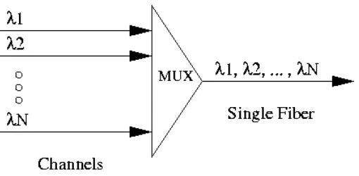
communication link can only run as fast as the highest possible electronic data rate (in the range of gigabits per second). To alleviate the electro-optic bottleneck, wavelength division multiplexing (WDM) has been proposed as a way to efficiently utilize the bandwidth of fiber. In WDM, the tremendous bandwidth of the fiber is divided into multiple non-interfering wavelengths, also known as channels. Each channel is a separate communication link that can be operated at lower electronic speeds. As shown in Figure 1.1, multiple channels can be multiplexed and transmitted simultaneously over a single fiber. In this manner, WDM provides an elegant solution to the electro-optic bottleneck problem. The amount of utilized bandwidth in WDM networks continues to increase as research leads to higher electronic speeds and greater number of available channels. Electronic speeds of 10 gigabits per second (OC-192) are now readily
Figure 1.1: Wavelength Division Multiplexing (WDM)
1.3 Motivation
An increasingly important capability for high-speed networks is the ability to provide multicast communication. In multicasting, a message is transmitted from a single source to multiple destinations. Multicast communication has a variety of applications which include audio/video conferencing, software/audio/video distribution, and
distributed data processing.
This thesis examines the problem of multicasting in an optical burst switched WDM ring network. The motivation is that optical SONET/SDH networks have been widely deployed in rings and used as metropolitan area networks (MANs).
Situations can arise where the simultaneous multiple transmissions on different channels are intended for a single destination receiver. This situation is known as a receiver collision. We examine various protocols for a ring network that address the issue of receiver collisions and evaluate how it affects network performance. The performance of the protocols is measured by simulation.
Optical burst switching is a relatively new switching technique that combines qualities from two well known switching techniques: packet switching and circuit switching. It is intended for use in networks where the traffic can be characterized as bursty. Thus, optical burst switching is suitable for Internet and World Wide Web traffic, which can be characterized as bursty.
1.4 Thesis
Organization
The thesis is organized as follows. In Chapter 2, we introduce multicast communication and the various topologies that implement multicasting. We will also examine some related work that deals with multicasting in a broadcast-and-select
network with a star topology. Chapter 3 provides an overview of optical burst switching. In Chapter 4, we introduce the network model used in our simulations. Chapter 5
Chapter 2
Background and Related Work
In this chapter, we first explore multicasting applications and present some arguments for supporting it at the WDM layer. Next, we introduce the various network topologies considered for multicasting: mesh, ring, and broadcast-and-select. We discuss the benefits of multicasting in a ring and broadcast-and-select network. Then we
examine some recent literature that is related to this thesis. We conclude with the differences between our research and the related work.
2.1 Multicast
Communication
As we have previously noted, multicast communication has many applications which include audio/video conferencing, software/audio/video distribution, and
There has been a tremendous amount of research over the years in the design and analysis of IP multicast protocols [3,4]. The MBone network is an example of an IP multicast implementation [5]. ATM networks have also been designed to provide multicast services with Q.2971 signaling [6].
2.2 Multicast Support at the WDM Layer
Since multicasting has already been developed and implemented in IP and ATM networks, it is reasonable to ask why support for multicast communication in WDM networks is needed. One compelling reason is that since light can be split, it is
advantageous to perform multicasting in the optical domain to avoid the opto-electronic conversion. IP and ATM multicast protocols copy packets/cells in the electronic domain requiring a conversion from optics to electronics back to optics (O-E-O). The O-E-O conversion significantly impacts end-to-end delay. WDM multicast also provides data rate transparency within the network. Another reason is that the WDM layer can acquire knowledge of the physical topology, which allows for more efficient multicast trees. For these reasons, multicasting at the WDM layer can be done cheaper (less equipment required) and more efficiently (lower delay, less number of hops) than at the network layer.
2.3 Topologies for Multicasting
2.3.1 Mesh Networks
Current mesh WDM networks use wavelength-routing. In wavelength-routed networks, transmissions are routed optically along a path from the source to the destination. This path is known as a lightpath. Lightpaths are used for point-to-point communication. An extension of the lightpath, known as a light-tree, is proposed for point-to-multipoint communication in [7]. Multicasting in wavelength-routed networks can be accomplished using multiple lightpaths or a single light-tree.
Research in multicasting for wavelength-routed WDM networks generally focus on efficient multicast routing algorithms. These algorithms are usually complex and the optimal solution has been proven to be NP-Hard [8]. Once the multicast tree is
constructed, then another algorithm is required to efficiently assign wavelengths across each of the links. Wavelength assignment is also a complex problem due to the
wavelength-continuity constraint. This constraint states that a transmission must use the same wavelength along the entire path. For this reason, wavelengths must be assigned so that no two transmissions use the same wavelength along the same link. The effects of the wavelength-continuity constraint can be reduced by using wavelength converters. Wavelength converters are capable of converting an input wavelength to a different output wavelength. However, they significantly add to the cost of the network and must be placed at strategic points in the network. Using wavelength conversion adds
Another multicasting issue in wavelength-routed networks is the optical power budget. A beam of light can only be split a limited number of times before it needs regeneration. This requires optical amplifiers which can significantly add to the cost of the network. Other problems to consider are looping, multiple transmissions, and topology changes. Because of all the above issues, multicasting in wavelength-routed networks is an extremely complex problem.
Mesh topologies are generally considered to be more robust and scalable than ring or broadcast topologies. Thus, mesh networks are well-suited for wide area networks (WANs). As optical technology progresses, they will become less costly and easier to implement.
2.3.2 Ring Networks
In comparison to mesh networks, ring networks have several features that make it more suitable for multicast communication. The primary advantage is that routing in ring networks is much simpler. Each node can assume that a transmitted packet is able to reach all destinations, since all other nodes are located along the ring path. Therefore, multicast algorithms for a ring topology normally require only a small amount of state information to be kept. They also employ simple data structures which are easy to maintain. In fact, for a unidirectional ring, the routing path is fixed and maintenance of a data structure for multicast routing is unnecessary.
unidirectional WDM ring networks for use in MANs. The detailed network model is presented in Chapter 4.
2.3.3 Broadcast-and-Select Networks
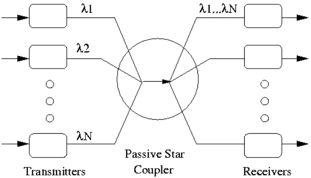
Another optical network well-suited for multicasting is a broadcast-and-select WDM network. In a broadcast-and-select network with a star topology, the nodes are connected together by a star coupler (see Figure 2.1). Each node is configured with a number of transmitters and receivers. In order to reduce cost and complexity, tunability is generally provided only at either the transmitters or receivers. We define a network that has fixed transmitters and tunable receivers as FT-TR. Alternatively, we define a network that has tunable transmitters and fixed receivers as TT-FR.
In a broadcast FT-TR network, a message is simultaneously transmitted to all nodes in the network on a specific channel. Any node can receive the transmission by tuning its receiver to that channel. Because of tuning delays, receivers must know the frequency of the transmitted message before it arrives. Consequently, some coordination between the source and destination is required. Just as in a ring network, multicasting is simplified since a multicast routing algorithm is not required.
Broadcast-and-select networks are difficult to scale and are most frequently implemented in a LAN environment.
2.4 Related Work
Early research on access protocols for optical networks focused on scheduling point-to-point transmissions. In [9], the paper studies access protocols for unicast transmissions over an OBS WDM ring. Our research uses the same general architecture and extends it for point-to-multipoint communication. More recently, there have been studies on scheduling multicast traffic in optical broadcast WDM networks [10-13]. We explore several of those papers below. Research on multicasting in optical burst switched WDM networks is still in its infancy. We discuss a recent paper on multicasting in an OBS WDM network.
2.4.1 Multicasting in Broadcast-and-Select Networks
destinations have received it. Each node is equipped with a tunable transmitter and tunable receiver (TT-TR). Nodes must obtain permission to transmit by sending a request to a centralized scheduler located on the broadcast star. This is done via a dedicated control channel. The scheduler coordinates the transmission by sending messages to the transmitter and receiver on a second dedicated control channel. Throughput performance is increased by introducing random delays between
retransmissions instead of continuous retransmissions. Another improvement studies conflict when a receiver has to choose from multiple messages. It is shown that a receiver algorithm which selects the message with the minimum number of recipients performs better than random selection. We note that the algorithms assume that the transceivers have low (nanosecond range) tuning delays. Large tuning delays would affect the efficiency and performance of the system.
In [12], an algorithm is proposed to minimize the schedule length for multicast transmissions based upon a fixed traffic matrix. Each node is equipped with a fixed transmitter and tunable receiver (FT-TR). The physical receivers are partitioned into a set of virtual receivers, where each physical receiver in the same set behaves identically. The tuning delays of the receivers are assumed to be non-negligible. The proposed solution divides the problem up into two parts. The first part deals with efficient
Another study of partitioning multicast transmissions is [13]. It is shown that the receiver waiting times can be reduced by partitioning and using a simple scheduling algorithm. A comprehensive survey of various protocols and algorithms used in WDM broadcast networks is provided in [14].
2.4.2 Multicasting in Optical Burst Switched WDM Networks
2.5 Ring
and
Broadcast-and-Select Networks Comparison
Chapter 3
Optical Burst Switching
Optical burst switching (OBS) is a switching technique introduced to support bursty traffic in an optical network. The motivation for using OBS is that much of the increased bandwidth demand is due to IP/TCP data traffic, which can generally be characterized as bursty. More specific to our problem, many multicasting applications such as video conferencing and video distribution are very bursty. In this chapter, we examine the problems with current switching techniques (i.e. circuit switching and packet switching) in the context of supporting bursty traffic in optical networks. Then we
discuss optical burst switching in detail. We conclude this chapter by describing various methods of signaling proposed for optical burst switching.
3.1 Circuit
Switching
round trip delay, since all nodes along the path must acknowledge that it is able to support the lightpath. This delay can be significant depending on the distance and number of hops between the source and destination nodes. During the setup delay, the intermediate nodes must reserve enough resources to support the lightpath. After the transmission is completed, the lightpath must be torn down. Due to the lightpath establishment and teardown overhead, circuit-switching results in low bandwidth utilization if the length of communication is short.
We may reduce the setup and teardown overhead percentage by keeping the connection up, and transmitting bursty traffic for a long duration. However, bursty traffic implies that there are a series of ON-OFF periods where the traffic is continuous during the ON periods and no traffic is present during the OFF periods. During the OFF periods, the bandwidth allocated to the lightpath cannot be used by others. This method also results in low bandwidth utilization.
3.2 Packet
Switching
Optical buffering currently consist of loops of fiber known as fiber delay lines (FDLs). FDLs are very costly and therefore infeasible to implement into all routers and switches.
Packet switching is widely used in electronic IP networks. It has proven to be a robust, scalable, and flexible technology. However, it will require decades in developing optical technology to successfully support photonic, packet switched networks.
3.3 Optical
Burst
Switching
Optical burst switching is designed to provide the desired functionality from both circuit switching and packet switching. In OBS, the unit of transmission is a burst. We define a burst as a collection of data packets. Bursts can be of variable length and may contain IP datagrams, ATM cells, or some other arbitrary type of data traffic. Prior to transmitting a burst, the source node sends a control message. This control message performs functions similar to a packet header in packet switching. The source node then transmits the burst shortly afterwards without waiting for an acknowledgement of the control message. Theoretically, a burst can be of indefinite length. In this manner, OBS resembles circuit switching except that lower setup delays are incurred. Bursts can also be very short, which would then resemble packet switching.
3.3.1 Control Message
switching, the control message is signaled out-of-band on a dedicated control channel similar to circuit switching. Currently in optical networks, control information must still be process electronically. A dedicated control channel, which is referred to in literature as a data communication channel (DCC), allows for signaling to be done electronically while the data channels remain completely in the optical domain. We note that a transmitted burst will be dropped if a node cannot fulfill the request due to conflicts.
3.3.2 Offset
In OBS, the period of time between transmission of the control packet and transmission of the burst is defined to be the offset. The purpose of the offset is to allow intermediate and destination nodes to have sufficient time to process the control message and setup the switch fabric prior to the burst arrival. By using the offset, bursts can be switched in the optical domain even though control information is processed
electronically.
3.3.3 OBS Schemes
3.3.3.1 Tell-And-Go (TAG) and Tell-And-Wait (TAW)
In TAG, the burst is sent immediately (i.e. offset is equal to zero) after the control message. Intermediate and destination nodes must buffer the burst using fiber delay lines, while processing the control message. TAG is similar to a method developed in ATM networks called ATM Block Transfer [6]. TAG results in a very short delay. However, burst drop probability is higher in TAG than in other schemes for networks without optical buffers.
We compare TAG with the tell-and-wait protocol, which resembles a circuit setup. In TAW, the source node sends a request and must wait to receive an
acknowledgement from the destination before transmitting the burst. Burst dropping is prevented but the delay is increased to at least the round-trip propagation time between the source and destination nodes. A performance analysis of TAG and TAW is provided in [17].
3.3.3.2 Just-In-Time (JIT) and Just-Enough-Time (JET)
In JIT, the offset is calculated based on an estimate on the number of hops and switching times of the intermediate nodes. The implementation of JIT has many similarities to setting up a circuit including explicit setup/teardown messages. JIT uses signaling acknowledgements, retransmissions, and timers to operate properly and efficiently. However, since bursts are still transmitted before a connection
Setup, Call_Proceeding, Connect, Release, and Release_Complete. The JumpStart and MONET projects are two examples that use JIT signaling [18,19].
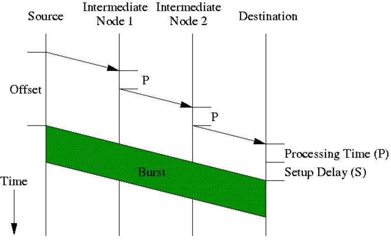
In the JET protocol, the offset is calculated to include the processing delays and setup delay at the intermediate and destination nodes (see Figure 3.1). We define h to be the number of hops and Pi to be the delay incurred in processing a control message for node i. We define S to be the delay in setting up a destination node to receive a burst. The offset calculation for JET is expressed as
) 1 . 3 ( 1
∑
= + = h i i S P offset JETNote that the number of hops, h, is required for calculation of the JET offset. In mesh networks, calculation of the number of hops may be quite complex. However, since we are dealing with ring networks, this calculation is simple. This can be accomplished by numbering the nodes in an ordered traversal around the ring. This information needs to be delivered to a node only once during node setup.
As seen in Figure 3.1, the burst is not delayed at intermediate nodes and
consequently can be delivered to the destination node without any optical buffering. We use the JET offset calculation for our simulations because it offers the shortest offset delay without the use of fiber delay lines.
Figure 3.1: JET Offset
3.3.3.3 Only-Destination-Delay (ODD)
Chapter 4
System Model
4.1 Ring
Architecture
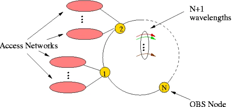
We consider a unidirectional WDM ring network of N nodes interconnected by fiber as shown in Figure 4.1. This ring is considered to be a backbone metropolitan area network, where each node is attached to several access networks. The fiber has the capacity to support C wavelengths where C = N + 1. N wavelengths are reserved for data transmission and the remaining channel is dedicated for transmission of control
information. Each of the N nodes is assigned a unique wavelength that it will use for burst transmissions. As a result, wavelength assignment needs to be performed only once during initial setup. We will denote the assigned wavelength as a node's home
wavelength. Note that the control channel is also on a unique wavelength, but it is shared by all nodes.
Figure 4.1: Architecture of OBS Ring with N Nodes
4.2 Node
Architecture
The architecture of a single OBS node is shown in Figure 4.2. The node's primary operational structures and their primary purpose are listed below.
• Scheduler: selects the next queue for transmission
• Control Module: processes incoming control frames
• Transmit Module: performs burst transmissions
• Receiver Module: operates the tuning of the receiver for reception of a burst
Each node is equipped with a single, dynamic, second-generation optical add-drop multiplexer (OADM). An OADM allows the node to selectively drop or add
wavelengths. Any wavelengths that are not dropped, will bypass the node optically. The control wavelength is always dropped, since each node is required to process every control frame from the control channel. The dropped control wavelength contains control frames that are processed by the Control Module. The operation of the control
wavelength is described in the next section. Once a control frame has been processed, it is reintegrated into the outgoing signal. A wavelength containing data that is destined for this node can also be dropped and processed by the Receiver Module. All other
wavelengths can bypass the node optically, without needing electronic termination. A node's home wavelength is also dropped so that new bursts may be introduced into the signal by the Transmit Module.
ratio is 50:50 [1]. We are dealing with a relatively small number of nodes in a multicast group, so this ratio should not cause any attenuation problems. However, if the optical power budget is limited, splitters with different splitting ratios can be used so that more power is returned to the signal continuing onto the next node.
Each node is also equipped with a pair of transceivers. The first pair is used for data transmission and is comprised of a fixed transmitter and tunable receiver (FT-TR). The fixed transmitter is tuned to the node's home wavelength. Each node is provided a home wavelength in which no other node can transmit on. This prevents collisions from occurring during transmission of a burst. The tunable receiver has the flexibility to tune to any of the data wavelengths. When a node wishes to receive a burst, it tunes its receiver to the transmitting node's home wavelength. The second transceiver pair is a fixed transmitter and fixed receiver that is tuned to the control wavelength.
4.3 Control
Wavelength
Operation
4.3.1 Control Wavelength and Control Frame Structure
Optical burst switched nodes communicate with one another by using the control wavelength. The control wavelength carries a sequence of control frames that
continuously circulate around the entire ring. Each of these control frames are divided into N slots. Each slot contains basic burst information (e.g. destination address, length of a burst, offset) for a particular node. Depending on the protocol used, there may be other specialized fields such as burst identification numbers, sequence numbers, tokens, and acknowledgements. Protocols may choose to use a single control frame for the entire ring or multiple control frames. In our work, we consider the case where the control frames are transmitted back-to-back around the ring. This enables the nodes to have immediate access to the control channel at all times. A drawback to having back-to-back control frames is that each node is required to perform more processing. Since we are implementing simple protocols, the node should be capable of handling the additional processing without much difficulty.
4.3.2 Sending and Receiving Burst Information
When a control frame arrives at a node, it is processed by the Control Module. First, it scans the entire frame to determine whether there is an incoming burst
accept one burst and reject all others. For reliability, some protocols may require that the Control Module insert a negative acknowledgement into the control frame if a burst cannot be successfully received.
Next, the Control Module consults the Scheduler to check if there exists an outgoing burst that is ready for transmission. If so, the necessary information for that burst is written into the appropriate control slot. If there is no burst for transmission, the appropriate control slot can be initialized to indicate no transmission.
4.3.3 Control Processing Delay
With respect to a burst transmission, a particular node may serve one of three roles: source node, intermediate node, and destination node. As a source node, it marks its slot in the control frame, prepares a burst for transmission, and inserts the burst into its home wavelength at the appropriate time. As an intermediate node, it allows the burst to bypass the node without any interference. As a destination node, it terminates the burst by configuring the OADM to drop the wavelength to receive the burst. In our
Chapter 5
Multicast Access Protocols
In this chapter, we examine various access protocols developed for multicasting over an OBS ring. First, we review the decisions made when initially designing the protocols. We then discuss how contention is resolved and any assumptions that were made. A detailed description of each protocol concludes the chapter.
5.1 Design
Choices
5.1.1 Algorithm Complexity
When initially designing the multicast access protocols, our main goal was to develop protocols that used simple algorithms. We wanted to avoid complex data
5.1.2 Fairness
Fairness is an important characteristic of a protocol. Whenever possible, we consciously made decisions that would intuitively create a fair protocol. For example, all the protocols serve their queues in a round-robin fashion. This avoids the issue of
starvation that can occur in priority queue systems. When a collision occurs, a node randomly chooses a burst to receive rather than a priority-type scheme. We note that these decisions may potentially have some negative effects on some performance measures. In [11], it was shown, for a broadcast star WDM network, that selecting the multicast message with the least remaining nodes offered better performance than random selection.
5.1.3 Distributed versus Centralized
We chose to develop only distributed protocols. Distributed protocols are
generally more robust than centralized protocols since there is no single point of failure. A distributed system spreads the processing load out among all nodes. This is
accomplished by having each node run a separate but identical copy of the protocol. The main disadvantage with distributed protocols is that scheduling is generally less efficient. Since each protocol can only operate based upon local information, it is more difficult to avoid collisions when transmitting bursts. For this reason, a distributed protocol may only be able to achieve local optimum points. Protocols may be required to use
5.1.4 Reliability
Another design choice was whether to study unreliable or reliable protocols. We define unreliable protocols as those that do not guarantee successful delivery of a burst. This is similar to best-effort IP or UDP service. However, we note that packets are delivered in-order within our OBS ring architecture. On the other hand, reliable
protocols ensure that a burst will be successfully received by all destinations. Reliability is ensured through use of acknowledgements, retransmissions, and timeouts. This is similar to TCP.
It can be argued that unreliable protocols should be used at the lower layers. If reliability is needed, the higher layer protocols can provide it. The tradeoff is that this dependence on the higher layers will increase the overall delay. Higher layers cannot explicitly know that a packet has been dropped and must depend on timeout mechanisms. In addition to the timeout delay, higher layers incur a larger propagation delay since the dropped packets must be retransmitted from the original source. We investigate both unreliable and reliable protocols in our work.
5.1.5 Preemptive versus Non-preemptive
5.1.6 Transceiver Tunability
Transceiver tunability is an important factor that affects the design of a protocol for WDM systems. Tunability can be provided at either the receivers, transmitters, or both. Systems with fixed transmitters and tunable receivers (FT-TR) must deal with contention when data on different wavelengths are destined for the same receiver. Systems with tunable transmitters and fixed receivers (TT-FR) must deal with collisions when two transmitters wish to transmit on the same wavelength. Systems with tunable-transmitters and tunable receivers (TT-TR) must deal with contention on both sides. Tunable transceivers generally cost more than fixed transceivers [21]. In our
architecture, we use FT-TR.
5.1.7 Synchronization and Fixed Sized Slots
Synchronization is often used in multicast access schemes to improve efficiency. They are popular when scheduling multicasts in broadcast-and-select networks.
5.2 Collision
Resolution
One of the primary responsibilities of access protocols is to resolve issues arising from contention of resources. We refer to this as collision resolution. We identify two types that occur in WDM systems: contention for a wavelength when transmitting a burst, and contention at a destination when receiving multiple bursts that overlap in time. For our purposes, we denote the first type as a transmitter collision and the second type as a receiver collision. We omit a third type, contention for a wavelength during wavelength-routing, because it is not relevant to our OBS ring architecture.
In our OBS ring, transmitter collisions are avoided since each node has a single transmitter and a unique wavelength for transmitting. However, this issue may arise in the case of multiple transmitters and/or sharing of wavelengths (see section on Future Research in Chapter 7).
Since each node is equipped with only a single receiver, receiver collisions may occur quite frequently in our architecture. The problem is magnified when multicasting, since each burst has multiple destinations. Even if a node is equipped with multiple receivers, a receiver collision can still occur whenever the number of wavelengths exceed the number of receivers.
5.3 Assumptions
We have stated that a burst can be comprised of many IP datagrams, ATM cells, or some other type of data traffic. We will assume that there is a method of grouping packets together so that they can be recovered after the burst arrives at the destination. We envision the capabilities to be similar to the Adaptation Layer 2 (AAL2) in ATM networks. See [6] for a description on AAL2.
We realize that any such method will require additional overhead that will affect network performance characteristics such as throughput, delay, and channel utilization. However, since each protocol must incur this overhead, we can still make comparisons on the relative performance of each protocol. In addition, the ratio of the overhead to payload in a burst for our simulations is very small. As a result, the effect of the overhead on performance should be minimal. To ensure that the ratio of overheads to payload in OBS are small, we introduce a parameter known as MinBurstSize. The MinBurstSize specifies the minimum length of a single burst. If a particular transmit queue does not contain enough data to meet the MinBurstSize, the queue is bypassed for service.
We also introduce the parameter, MaxBurstSize, which specifies the maximum length of any burst. When a queue is being serviced, packets are added to the burst until either the queue is empty or the MaxBurstSize is reached, whichever comes first. To further simplify the protocols, we assume that individual packets are not split. That is, no segmentation and reassembly of individual packets occur within the OBS ring. Thus, a packet is excluded from a burst if its addition will result in a burst that exceeds
5.4 Access
Protocols
In this section, we describe the four protocols proposed in this thesis for multicasting in our OBS ring. Three of them (Persistent, Unicast Token, Multicast Token) are reliable multicast protocols and one (Unreliable) is unreliable. The protocols explore two opposing paradigms used in multicasting. One is multicasting by sending only one transmission. Multicast Token, Unreliable, and Persistent are examples of this. These protocols attempt to conserve bandwidth. Another view is that multicasting can be accomplished by sending a separate unicast transmission to each destination. Unicast Token is an example of this.
All of the following protocols are distributed. As a result, each node executes an identical copy of the protocol. For all protocols, the buffer at a node is arranged in logical queues with each queue representing a particular multicast group. Upon entry into an OBS node, packets coming from the access networks are placed into one of these queues. The offset is calculated by using Equation (3.1) for all protocols. Table 5.1 summarizes the attributes of each protocol.
5.4.1 Unreliable
Source Node Operation
Prior to transmission, the scheduler selects the next multicast queue that contains data greater than or equal to the MinBurstSize. When the node's transmitter is available (i.e. not busy transmitting a burst), it waits for the next available control frame. When the control frame arrives, the node marks information about the burst in its own slot. This information includes the multicast address, burst duration, and the offset. The node then waits for a period of time equivalent to the offset value, before transmitting the burst.
After burst transmission, the buffer memory for that burst is freed. The node also performs maintenance of its own control slot by clearing out any information related to previously transmitted bursts.
Destination Node Operation
Whenever a control frame arrives, the node examines the entire frame to determine which slots, if any, contain burst information intended for it. This is performed by determining the multicast address of each slot and checking if it is a member of that multicast group. If the node is the destination of more than one slot, it randomly chooses one of the bursts to receive. The node does nothing if no slots contain information destined for it.
OADM to drop the appropriate wavelength and the receiver to tune to it. If a burst cannot be accommodated, the OADM does not drop the wavelength.
5.4.2 Persistent
The Persistent multicast protocol is designed to provide reliable service.
Reliability is accomplished via retransmissions and acknowledgements. In the Persistent protocol, retransmissions occur until all intended nodes have successfully received the burst. The scheduler services the multicast queues in a round-robin fashion. In the following subsections, we examine the operation of the source and destination node in detail.
Source Node Operation
greater than the last burst. In this fashion, the BIN can be viewed as a sequence number. We assume that the node has simple logic capable of dealing with minor issues such as wrapping and sequence number comparisons. We omit those details here since they do not affect the overall operation or performance of the protocol.
Next, the node waits for a period of time equivalent to the offset value before transmitting the burst. After the burst has been initially transmitted, the node then waits for the control frame containing the same BIN. This duration is equivalent to the round-trip time around the ring, which includes propagation and processing delays, minus the offset duration. When the control frame with the same BIN returns to the node, the array of nack bits are examined. If any nack bits have been set to true (meaning that at least one destination node did not successfully receive the last transmission), the burst is retransmitted using the same multicast address. The nack/retransmission process is repeated until all nack bits return false.
After successful transmission to all nodes, the memory containing the burst may be freed. The node also performs maintenance of its own control slot by clearing out any information related to the previously transmitted burst.
Destination Node Operation
accomplished by comparing the BIN in the slot with the BIN from the last successfully received burst from the source node. If the burst has already been successfully received, the node ignores that slot. Otherwise, the slot is a candidate burst for reception.
If the control frame contains a single candidate, the burst in that slot is selected for reception. If more than one candidate exists, the node randomly chooses one of the slots to receive and sets the appropriate nack bits for all the other candidates to true. If the control frame contains no candidates, the node does nothing.
Once a slot has been selected, the node checks the availability of its receiver during the time period when the burst arrives. This time period is extended to include tuning latency of the receiver. If it can accommodate the burst, the node programs the OADM to drop the appropriate wavelength and the receiver to tune to it. If a burst cannot be accommodated, the OADM does not drop the wavelength and the node sets the nack bit for the slot to true.
5.4.3 Unicast Token
The Unicast Token protocol derives it name from the fact that multicast communication is actually performed via multiple unicast transmissions, one for each destination. In the following subsections, we examine the operation of the tokens, source node, and destination node in detail.
Token Operation
Tokens are carried in control frames which are located in specialized token fields and circulated around the ring. Each node examines every incoming control frame for any available tokens, which are then captured by removing the token from the control frame. The only exception is that a node never captures its own token. Captured tokens are placed in the node's token queue. They are released by writing the tokens back into a control frame. Once the scheduler has serviced a token, it is released immediately after the burst is transmitted.
Source Node Operation
We note that even though Unicast Token performs multicasting as multiple
Prior to transmission, the scheduler selects the next token (representing a single destination node d) from the token queue. Next, the scheduler visits each of the multicast queues that node d is a member of. The packets in each of these queues are copied to a temporary storage area. If the length of the temporary burst is greater than the
MinBurstSize, the burst is scheduled for transmission. Otherwise, the token is released in the next available control frame and the burst is not transmitted.
When the node's transmitter is available, it waits for the next available control frame. When the control frame arrives, the node marks information about the burst in its own slot. This information includes the unicast destination, burst duration, and the offset. The node then waits for a period of time, equivalent to the offset value, before
transmitting the burst.
After every burst transmission, the node releases the serviced token and then attempts to free buffer memory. Memory can only be freed for packets that have been transmitted to all its destinations. To facilitate this, a pointer is kept for each member node in a multicast queue. A pointer for member node n indicates the last packet that was transmitted to node n. Pointers are updated after every burst transmission.
Destination Node Operation
The destination node performs maintenance of the control slot by clearing out any information related to transmissions intended for it.
5.4.4 Multicast Token
The Multicast Token protocol is designed to provide reliable service. Similar to Unicast Token, reliability is accomplished using tokens. In the Multicast Token protocol, each node's receiver is designated with a unique token. These tokens are circulated around the ring from node to node on the control wavelength. A source node must obtain all the tokens for the destination multicast group before transmitting a burst. The
scheduler services the multicast queues in a round-robin fashion.
By gathering all tokens before transmitting, the Multicast Token protocol uses the minimum of one transmission per multicast communication. For this reason, Multicast Token is optimal with respect to channel utilization. In the following subsections, we explain the operation of the protocol in detail.
Token Operation
Tokens are carried in control frames located in specialized token fields and
circulated around the ring. Each node examines every incoming control frame to check if it contains tokens needed for the next multicast transmission. If so, the tokens are
Deadlock Avoidance
Since each node obtains multiple tokens before transmission, Multicast Token must deal with the issue of deadlock. Suppose two nodes, s and t, require the same tokens, A and B, for its next transmission. If node s acquires token A and node t acquires token B, we have a deadlock situation. Both nodes will be waiting for a token that the other node is holding.
Multicast Token uses a simple algorithm to avoid deadlock. All the tokens in the OBS ring are given a logical order. For n tokens, they would be ordered {1,…,n}. We specify that nodes must obtain tokens for a multicast group in-order. For example, if a node needs three tokens numbered {1,4,7} for a multicast transmission, it must first grab token 1, then 4, and then 7. If token 4 appears in a control frame and the node does not already have token 1, the node is prohibited from capturing token 4. Nodes are allowed to obtain multiple tokens from a single control frame. In the previous example, tokens {1,4,7} can all be acquired if they are found within the same control frame.
Source Node Operation
all the required tokens, it can proceed to transmit the burst. All tokens in the node's possession are released after a burst transmission.
Since the tokens guarantee that no collisions will occur, the burst memory can be freed immediately after transmission. The source node also performs maintenance of its own control slot by clearing out any information related to the previously transmitted burst.
Destination Node Operation
Whenever a control frame arrives, the node examines the entire frame to determine which slot, if any, contains burst information intended for it. This is accomplished by determining the multicast address of each slot and checking if it is a member of that multicast group. If so, the node programs the OADM to drop the appropriate wavelength and the receiver to tune to it. Because tokens are used, at most one slot will contain burst information for the node.
Table 5.1: Protocol Summary
PROTOCOL RELIABLE OR UNRELIABLE METHOD OF RELIABILITY TRANSMIT METHOD
Unreliable unreliable none multicast
Multicast Token reliable tokens multicast Persistent reliable nacks/ retransmissions multicast
Chapter 6
Numerical Results
In this chapter, we present our simulation results of the four protocols. First we discuss the simulation parameters, how multicast groups are generated, and the arrival process. We compare the protocols in the following key performance areas: receiver throughput, overall packet delay, channel utilization, and fairness. Performance is measured for varying packet arrival rates.
6.1 Simulation
Parameters
Our simulated ring consists of 10 nodes and 11 channels. The ring utilizes 10 channels for data transmission and one channel for signaling. The nodes are equally spaced around the ring and separated by a distance of 5 km. Each data channel operates at 2.5 Gbps and the control channel operates at 622 Mbps. A single slot in a control frame is 100 bytes in length which is equivalent to a duration period of 1.29
the access networks. We varied the average arrival rate, MinBurstSize, MaxBurstSize, number of multicast groups, and multicast group membership to measure the
performance of the protocols.
6.2 Multicast
Group
Generation
For each simulation run, G multicast groups are generated in the following manner. Each node is assigned a number, pi, in the range (0,1), which represents the probability that a node would be a member of a multicast group. For each multicast group, a random number, r, is generated for each node in the ring. We use a
pseudorandom generator that produces numbers that are I.I.D. and uniformly distributed in the range of [0,1). If r < pi, then that node is included in the multicast group.
Typically, we use the value, pi = 0.5, for all nodes. We refer to this case as having
uniformly generated groups. The multicast groups are static, meaning that membership of a group does not change during the course of the simulation.
Figure 6.1: IPP State Transition Model
6.3 Traffic
Generation
We simulate traffic coming from the access networks into the OBS ring based on a continuous-time distribution known as the Interrupted Poisson Process (IPP) [22]. The state transition model is shown in Figure 6.1. IPP has two states: ON and OFF. During the ON state, packet arrivals occur at a rate of λ. During the OFF state, the arrival rate equals zero (e.g. no arrivals occur). The length of the ON and OFF periods are
exponentially distributed with means of 1/µ1 and 1/µ2 , respectively. The process
alternates between the ON and OFF states.
arrives before the OFF period begins. As a measure of burstiness, we use the c2 of packet inter-arrival times which is calculated by
) 1 . 6 ( ) ( 2 1 2 2 1 1 2 µ µ µ λ + + = c
where λ is the rate of packet arrivals during the ON period, 1/µ1 is the mean time of the
ON period, and 1/µ2 is the mean time of the OFF period. It has been experimentally
shown that the c2 of IPP is very close to the c2 of IPPm [9]. By using the mean packet inter-arrival time, we can derive an expression for the average arrival rate (AAR).
) 2 . 6 ( 2 1 2 µ µ µ γ + × = AAR
where γ is the arrival rate equal to 2.5 Gbps. If we are provided both c2 and AAR, we can solve for µ1 and µ2 from the equations above. Therefore, we can characterize the arrival
process by specifying the parameters c2 and AAR.
In our simulations, each node runs a separate but identical IPPm to generate traffic coming from its attached networks. For all simulations, c2 has been set to 20 and the AAR is varied. Incoming packets are randomly assigned to a multicast group.
6.4 Simulation
Results
6.4.1 Effect of Average Arrival Rate
We examined the effect of the average arrival rate on four performance measures: receiver throughput, overall packet delay, channel utilization, and fairness. In these simulations, we assumed a ring with 10 nodes and 9 multicast groups. The multicast groups are generated uniformly and contain a minimum of 2 to a maximum of 10 members. Although each node runs an identical arrival process, the traffic is heterogeneous due to the variation in multicast group membership.
Receiver Throughput
In Figure 6.2, we plot the receiver throughput of the four protocols for various arrival rates. We define receiver throughput as the number of bits successfully received by a node's tunable receiver over a period of time averaged over all receivers. As seen in Figure 6.2, the Unicast Token protocol achieves the best performance over the range of arrival rates. In fact, it achieves optimal receiver throughput performance for all arrival rates except at 400 Mbps. We define optimal receiver throughput as successfully delivering every incoming packet to all intended destinations. In our network, the optimal receiver throughput per node can be calculated by
0 200 400 600 800 1000 1200 1400 1600 1800 2000
0 100 200 300 400 500
Average Arrival Rate (Mbps)
Receiver Throughput (Mbps)
Unreliable Persistent Unicast Token Multicast Token
Figure 6.2: Receiver Throughput for N = 10 nodes, G = 9 groups (Uniform)
where g represents the number of multicast groups a node is a member of, G is the total number of multicast groups, and N is the number of nodes in the ring. The other protocols suffer as arrival rates increase. In fact, the reliable Multicast Token protocol performs worse than the Unreliable protocol for arrival rates above 150 Mbps. The Persistent protocol performs the second best and achieves optimal receiver throughput with arrival rates up to 300 Mbps.
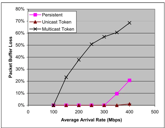
full. All protocols are susceptible to packet buffer loss and the probability of buffer loss increases as the arrival rate increases. We note that the amount of packet buffer loss is related to the average overall packet delay. Delay and buffer loss is discussed in the next section.
Overall Packet Delay
Packets traveling through the OBS ring incur two types of delay. Propagation delay is the amount of time it takes for the burst to travel from the source node to the destination node. Assuming a fixed path, the propagation delay, δp, is the same for all
packets traveling from the same source node to the same destination node. Specifically in our case, the propagation delay is the same for any two messages traveling the same number of hops. This is due to the fact that nodes in our ring are equidistant. Buffer delay, δb, is defined as the amount time a packet spends waiting in a source node's buffer
before it is sent in a burst.
We note a key difference in the delay measurement between the unreliable and reliable protocols. For unreliable protocols, there are no retransmissions and delay is measured regardless of whether the burst was successfully received. For reliable protocols, retransmissions may occur and delay is only measured for packets that are successfully received. Due to multiple transmissions of the same packet, a single multicast packet may experience different buffer delays to different destinations.
In Figure 6.3, we plot the average overall packet delay of the four protocols for various arrival rates. The results for the Unreliable protocol represents a lower delay bound for overall packet delay. That is, no other protocol using the same type of scheduler (round-robin with FIFO queue) can achieve better delay performance.
The Unicast Token protocol offers the best delay performance out of the group of reliable protocols. It compares favorably with the delay performance of the Unreliable protocol for all arrival rates except the highest at 400 Mbps. The Multicast Token protocol has the worst delay performance by far. This result is not entirely surprising, since a node must wait and acquire all tokens before transmitting a multicast burst.
In all the reliable protocols, we see a pattern where the delay is low (< 50
milliseconds) for the lower arrival rates. As the arrival rates approach a certain threshold, the overall packet delay increases dramatically. As shown in Table 6.1, this threshold occurs at different regions for each protocol. We denote this region as the initial area where the protocol can no longer maintain pace with the arrival rate. As seen in Figure 6.4, the threshold indicates the region where packet buffer loss begins to occur.
Table 6.1: Packet Buffer Loss Threshold for Reliable Protocols
PROTOCOL THRESHOLD RANGE
Multicast Token 100-150 Mbps
Persistent 300-350 Mbps
0 100 200 300 400 500 600 700
0 100 200 300 400 500
Average Arrival Rate (Mbps)
Overall Packet Delay (msec)
Unreliable Persistent Unicast Token Multicast Token
Figure 6.3: Overall Packet Delay for N = 10 nodes, G = 9 groups (Uniform)
0% 10% 20% 30% 40% 50% 60% 70% 80%
0 100 200 300 400 500
Average Arrival Rate (Mbps)
Packet Buffer Loss
Persistent Unicast Token Multicast Token
Channel Utilization
We define channel utilization as the percentage of time in which the channel is occupied for burst transmission averaged over all channels.
) 5 . 6 ( 1 1
∑
= × = Ni channel bandwidth fornodei
i node for rate bit r transmitte fixed average N n utilizatio channel
In Figure 6.5, we plot the channel utilization for each protocol at varying arrival rates. The Multicast Token and Unreliable protocols form a lower bound since each sends a multicast transmission only once. However, note that Multicast Token has lower channel utilization than Unreliable for higher arrival rates due to packet buffer loss. The
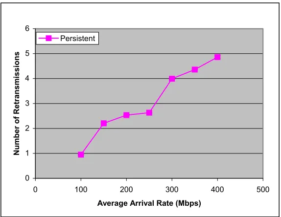
Persistent and Unicast Token protocols have the highest channel utilization, with Persistent having the fastest rate of channel utilization increase. In the Persistent protocol, higher arrival rates increase receiver contention, which results in more retransmissions. This is shown in Figure 6.6, which plots the average number of
Persistent retransmissions for various arrival rates. The increased retransmissions creates a problematic cycle by increasing receiver contention. Unicast Token has a linear
0% 10% 20% 30% 40% 50% 60% 70% 80%
0 100 200 300 400 500
Average Arrival Rate (Mbps)
Channel Utilization
Unreliable Persistent Unicast Token Multicast Token
Figure 6.5: Channel Utilization for N = 10 nodes, G = 9 groups (Uniform)
0 1 2 3 4 5 6
0 100 200 300 400 500
Average Arrival Rate (Mbps)
Number of Retransmissions
Persistent
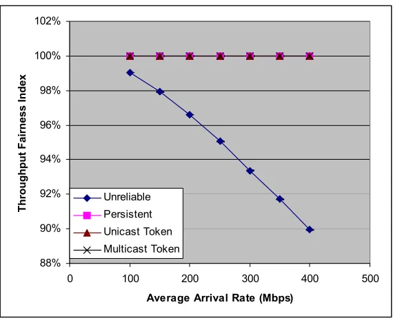
Throughput Fairness
We characterize a protocol as being throughput fair if the receiver throughput from a source node i to a destination node j does not depend on node's j location in the ring. In order to measure throughput fairness, we use the fairness index as proposed in [24]. First, we define the ratio Xij as the normalized throughput from node i to node j as
) 6 . 6 ( )
(fair receiver throughput fromito j ideal j to i from throughput receiver actual Xij =
The ideal receiver throughput from node i to node j is calculated by
) 7 . 6 ( ) ( 1 , 1 i N k k N i k k j g g k to i from throughput receiver g j to i from throughput receiver ideal − × =
∑
∑
= ≠ =where gk represents the number of multicast groups a particular node k is a member of, and N is the number of nodes in the ring. Then, the fairness index for node i can be expressed as ) 8 . 6 ( ) 1 ( , 1 2 2 , 1 × − =
∑
∑
≠ = ≠ = N i j j j i N i jj ij
X N X i node for index fairness
where N is the number of nodes in the ring. The fairness index has a range of [0,1] with a value of 1 (e.g. 100%) being completely fair. It has the desirable properties of being population size independent, scale independent, continuous, and dimensionless.
This results from the increased receiver contention at higher arrival rates. When contention occurs, the burst with the shortest distance between source and destination node has a distinct advantage. We illustrate this with the following example. Suppose node A and node B decide (at the same moment in time) to transmit a burst to node C, which would result in a receiver collision. Assume that node B is closer to C, and thus, has a lower propagation delay. Since the setup message from node B will arrive first, node C will choose to receive the burst from node B. Figure 6.8 shows the normalized receiver throughput from source node 1 to all other destination nodes for the Unreliable protocol (AAR = 400 Mbps). The normalized throughput decreases as the distance between the nodes increases.
Delay Fairness
We use the fairness index as described in the previous section and apply it to measure delay fairness. Here, the delay refers to the amount of time a packet spends waiting in the source node's buffer. We define the normalized delay, Xij , as
) 9 . 6 ( ) 1 ( , 1
∑
≠ = × − = N i j j j i j i j i delay delay N X88% 90% 92% 94% 96% 98% 100% 102%
0 100 200 300 400 500
Average Arrival Rate (Mbps)
Throughput Fairness Index UnreliablePersistent
Unicast Token Multicast Token
Figure 6.7: Throughput Fairness Index for N = 10 nodes, G = 9 groups (Uniform)
0 5 10 15 20 25 30 35 40 45
0 10 20 30 40 50
Destination Node Distance (km)
Normalized Receiver Throughput (Mbps)
Unreliable
80% 85% 90% 95% 100% 105%
0 100 200 300 400 500
Average Arrival Rate (Mbps)
Delay Fairness Index Unreliable
Persistent Unicast Token Multicast Token
Figure 6.9: Delay Fairness Index for N = 10 nodes, G = 9 groups (Uniform)
6.4.2 Tradeoff between Channel Utilization and Throughput/Delay
When comparing the performance of the reliable protocols, it is evident that there exists a tradeoff between channel utilization and throughput/delay. Unicast Token and Persistent both have much higher channel utilization than Multicast Token. They also exhibit superior throughput and delay performance.
tokens greater than or equal to TokensNeeded, or has collected the last required token for the multicast transmission. We refer to this new protocol as Modified Multicast Token. In essence, Modified Multicast Token partitions a multicast transmission into multiple group transmissions. The variable, TokensNeeded, determines the number of recipients (e.g. destinations) in a group transmission. We simulated an OBS ring with 10 nodes, 9 multicast groups, and 4 nodes per group. Figure 6.10 plots the receiver throughput of Modified Multicast Token for varying TokensNeeded from one (representing the unicast case) to maximum (representing the original Multicast Token protocol). Figures 6.11 and 6.12 plot the delay and channel utilization performance. As expected, delay and
throughput performance improves as TokensNeeded is decreased. Also, as a result of more transmissions, channel utilization increases as TokensNeeded is decreased.
200 300 400 500 600 700 800 900 1000
0 100 200 300 400 500
Average Arrival Rate (Mbps)
Receiver Throughput (Mbps)
1 token 2 tokens 3 tokens all tokens
0 100 200 300 400 500 600
0 100 200 300 400 500
Average Arrival Rate (Mbps)
Overall Packet Delay (msec)
1 token 2 tokens 3 tokens all tokens
Figure 6.11: Overall Packet Delay for varying TokensNeeded (Modified Multicast Token)
0% 5% 10% 15% 20% 25% 30% 35% 40%
0 100 200 300 400 500
Average Arrival Rate (Mbps)
Channel Utilization
1 token 2 tokens 3 tokens all tokens