The superposition of discrete-time Markov renewal processes with an application to statistical multiplexing of bursty traffic sources

The Superposition of

Discrete-Time Markov Renewal

Processes

with

an Application

to Statistical Multiplexing of

Bursty Traffic Sources

K. M. Elsayed

H. G.

Perros

Center for Communications

and

Signal Processing

.

Department of Computer Science

North Carolina State University

~/

/TR-94/15

The Superposition of Discrete-Time Markov Renewal

Processes with an Application to Statistical

Multiplexing of Bursty Traffic Sources

*

Khaled M. Elsayed

Harry G. Perras

Department of Computer Science

and

Center for Corrununications

and

Signal Processing

North Carolina State University

Raleigh, NC 27695-8207

Abstract

L~ this paper we introduce a methodology for approximately characterizing the su perpo sition process of J.V ~ 2 arbitrary discrete-time Markov Renewal Processes (MP2). The superposition process is also a ~..,,1RP with a state space that grows expo-nentially with N. We introduce the arbitraryanioff traffic source model as a special caseof the general~.For this special case, we devise an iterative algorithm which can be used to characterize the superposition process in a compact form. Subse-quently, a queueing model for a FIFO finite-buffer multiplexer with arbitrary anioff input sources is analyzed. We provide extensive numerical and validation results for the algorithms introduced in the paper. We also study the effect of some of the statistical properties ofanioff input sources on the multiplexer's performance.

1

Introduction

In this paper, we consider the problem of characterizing the superposition of multiple

discrete-time Markov Renewal Processes (IvfRP). A lot of research has been reported in

the area of characterizing the superposition process of renewal and Markovian processes.

However, to the best of our knowledge characterizing the superposition of MP~'s has not

as yet been adequately addressed.

Non-Markovian processes are more versatile since they can provide realistic models

of arrival processes in an ATMenvironment. However, the analysis of queueing systems

with non-Markovian input is considerably more complex than that with renewal and

Markovian arrival processes.

Cherry and Disney [1] studied the superposition of two continuous-time MRP's. The

structure of the interval process resulting from superposing two independent MRP was

characterized. The resulting stochastic process has a very large number of states which

limits the applicability of the model to two processes.

Korolyuk [6]introduced a mathematical model for the superposition of multiple

inde-pendent continuous-time lv1RP's. The model keeps track of the time each process spends

in the current state. This limits the model's applicability to cases where analytic

expres-sions for the sojourn times between states can be found. The author also introduced the

notion of

phase space lumping/

an aggregation process, in crder to red uce dimensionality

of the MF.P.

Following a similar methodology to the one presentedin [1]and[6],we characterize the

superposition of N

2

2independent discrete-time MRP's. The constructed superposition

is a 11R.P with a state space that grO\VS exponentially with N. Only small values of N

can be handled on a conventional computer. An aggregation method was developed in

the case of onloff processes, where the on and off periods have an arbitrary distribution.

Such a process is hereafter referred to as an arbitrary orr/off process. This aggregation

causes a distortion of the statistical properties of the original superposition. However,

the aoczregation works well in the case of Interrupted Bernoulli Processes. Finally, a

be,

FIFO finite buffer statistical multiplexer with N arbitrary onloff arrival processes was

analyzed. The analysis is non-standard due to the new model of the superposition of the

arrival processes.

Sohraby [8] presented innovative results on the tail beha~ior of a multiplexer with

infinite waiting room shared by multiple arbitrary

ani

off sources. For the case of

geneous sources, the model is valid only in heavy traffic. For the case of homogeneous

sources, the model can be used for all levels of multiplexer utilization. In the

heteroge-neous case, the asymptotic decay parameterisa simple function of the first two moments

of the on and off periods and peak rates. However, our results show that for the case

of a multiplexer with finite buffer, more parameters are needed than just the first two

moments of the on and off period lengths (when peak rate is equal to link speed).

The rest of this paper is organized as follows. In section 2, we first provide a quick

reviewofMarkov renewal processes and present some results from discrete-time renewal

theory. Wethen proceed to describe the methodology for characterizing the superposition

of multiple independent:MRP'

s.

In section 3, we present thearbitrary

onl

off source model.

A step-wise algorithm which uses aggregation in order to obtain a superposition process

ofarbitrary

onl

off sources with a manageable numberof statesisintroduced in section 3.2.

Insection 4, a finite buffer FIFO statistical multiplexer shared by multiple arbitrary on/off

traffic sources is introduced and analyzed. Insection 5, we present extensive validation

results of the algorithms presentedin this paper. Insection 6, we examine the effects of

some of the parameters of an arbitrary orr/offsource on the performance of a statistical

multiplexer. Section 7 gives the conclusions ofthis papero

2

The Superposition of Multiple Independent Discrete-time

Markov Renewal

Processes

2.1

A Revie-w of Discrete-fune Markov Renewal Processes and Some Basic

Results from Renewal Theory

A Markov renewal process GvfRP) is a stochastic process which moves from one state to

another with a random sojourn times which has a distribution that depends on the state

being visited as well as the next state to be entered. The successive states visited by the

MRP form aMarkov chain. Let 3 be the state space of an :tvIRP.

n E Z+I and 0

==

To ::;T_{1 ::;} T2 · · .,isa discrete-time:MRP withstate space

:=:

if

for all T,k E Z+ and z E 3. Let us further assume that (X, T) is time-homogeneous;

that is P {Xn+1

==

y,Tn+1 - Tn

==

kl"-Yn

==

x}

==

G(x,y,k) independent of n. The family

of probabilities G

==

{G(x,y,k): x,y E 3,k E Z+} is called a discrete-time semi-Markov

kernel on 3. The process (X) is called the associated semi-Markov process (S1vfP) of the

11RP (X, T). Whenever appropriate, we would use the termS1vfPinplace of:MRP.

The sum

p(

z ,y)

==

Ek~O G(z ,y, k) is not necessarily equal to one, but

p(

z ,y) ~ 0and

L:

_lIEs p( x , y ) must be equal to one. The p(x,y) are in fact the transition probabilities for some Markov Chain with state space E and probability transition matrix P

==

[p(x,y)].

We now review some basic results from renewal theory that will be used below to

construct the superposition process. Let f(k), 0

<

f(k)

<

1, k ~ 0,be a probability mass

function. Let w

==

~k=O f(k),

a

<

l.k' ~ 1, and

Sf

==

~k==O kf(k). Let F(k) == ~7=o f(l), be

the associated cumulative probability density function of length up to k. The probability

~~:.;-~ssruncrio.. ofthe residual life-timeis given by :

....

[W-F(k-l)]

f(k)=w M ' k=1,2, .. · (1)

Note

that whenw is

equal to

1,we get

the known

results for discrete-time renewal theory

[9].

2.2

Characterization of The Superposition Process of Multiple

Indepen-dent Markov Renewal

Processes

Consider pI

2:

2independent discrete-time}ARP's. Each individual MP,j)iis characterized

in terms ofc.semi-Markov kernel Gi ==

(gi(

z ,y"Ic)]defined over the set of states 1,2,· · ·Nil

N,

>

1. In order to characterize the superposition process, we have to define the states of the process and then for each state find the distribution of the sojourn time between the

state and

any

other directly accessible state of the superposition process.

In [1] the superposition state descriptor is a vector consisting of the current state of

each component process and the time each process has spent in its current state since its

last transition. It is clear that such a characterization results in an enormous state space,

since the time a component process spends in a state can be quite large especially when

some of the functions

s. (

x, y,k )have a long tail.

To show how our superposition is constructed, let us assume for the moment that only

one particular process, say process i, has just experienced a state transition and another

process j, j

#-

i, did not change state at that instant and that it is in state Xj. Let T(xj)

be the time that process j has spent so far in state Xj. Due to the independence of the

two processes, the distribution ofT(xj) will be equal to the distribution of the life-timein

state Xj. The time

T'(xj)

that it takes process j to undergo a state change would have a

distribution equal to the residual time distribution at state Xj.

This is illustrated through the example given in figure 1. At the instant marked

observation Instant,process 1 makes a state transition from state 2 to state 3. The distribution

of time until processes:2 and 3 e.oerience a state transition, T'(

X2)

andT'(

X3)

respectively,

i.3 appro~<i:-n.a.tel)/ equal to the residual life-time distribution in state 2 and state 1 of each

process respectively. Thisis true when we take all possible realization of the above event

and

assuming

that all processes are independent.

We define the superposition state at instants when one or more of the individual

processes experience a state transition. The superposition state is described by the tuple

[(Xl,tl),(X2,t2),···,(XN,tN)]

where Xi E

{1,2,··.,N

i } is the state of process i observed

immediately after a transition occurs, and ti E {O, 1} indicates whether process i has

changed state or not, with ti

==

1iffprocessi has changed state.

The state space E of the superposition process is givenby

Note that ~~1ti =I- 0 because the superposition process is observed immediately after a transition occurs. The number of states in the superposition processisobviously equal to

Ooservalion Instant

2

L

Process1

. . . - - - .I. . . - - - . Process 3

Process2

L

1"(IJ

_ _1_---. :

_---~ I~_

Io....---L---l

2 2

Figure 1: The distribution of residual life-time for a process not experiencing a state change.

In order to fully characterize the superposition process as a MRP, we must obtain the

distribution of the time it takes the :t\,fr.J> to move from a stateu to state v, whereu,v E ::::

and v is directly accessible from u, Let the probability of going from u to v in k slots be

denoted byq(1.£,1),k). ThenQ = [q(U,11, k)

J

isthe semi-Markov kernel of the superposition

process. We now proceed to calculate the functions q(u, v,k).

Let9i(

x,

y,k)be the residual life-time probability mass function associated with

s.

(x,

y,k)

which is calculated using equation 1. Also, let Gi(x,k)

=

:L~~1

:L7=1

9i(X,y,1),be the

cu-mulative distribution function of sojourn time up to slot k in state z for process i, and

G

i (z ,k) = :L~1

:L7=1

9i(z ,

v,

l)be similarly defined for the functions 9i(z ,y,k).

The function q(u,v,k) depends on the values of

(Xi(U),ti(u))

and

(Xi(V),ti(V))

for all

processes i, where

(Xi(S), ti(S))

isthe state of process i when the superposition isin state s.

We assume that the transition from state u to state v would take place in kslots and then

proceed to calculate the probability of this event to occur. Consider an arbitrary process

i, based onthe values of ti(

u)

and

ti(v ),

the following four distinct cases are possible:

1-

ti(

u)

=

ti(

v)

== O. In this case we have

Xi(

u)

==

Xi(

v),

i.e. process i does not change state in either state u orv. The probability of such an event to occur for process i is

approximately given by <p;(u,v,k)

=

1 - G;(x;(u),k), which is the probability that the residual life-time in state Xi(u)is greater than k.

11-

tie

u) =

a

and

tie

v) = 1.Inthis case processi changes state atvbut not atu, Since process

i has not changed state at u, the probability that this event occurs is

1Ji(

u, v,k)

==

9;(X;(u),x;(v),k),which is the probability that the residuallife-tirne in state Xi(U) is

equal to k.

111- ti(

u)

==

1 and ti(

v)

== O. In this case process i changes state at

u

but not at

v.

The probability that this event occurs is <Pi(u,v,k)

==

1 - Gi(x,:(u),k), which is the

probability that the sojourn time in state Xi(u) islonger than k.

IV- ti(U)

==

ti(V)

==

1. In this case process i changes state at both u and v. The

proba-bility that this event occurs is given by cPi(u,v,k)

==

9i(Xi(U),Xi(V),k), which is the

probability that the sojourn time from state Xi( u) to state

Xi(

v)isequal to k slots.

Thus, due to tile in.dependence of the component processes, we have the result

N

q(u,v,k)

==

II

cPi(u,v,k)

i=1

for all u; v E

:=:

and k E Z+~

(2)

We now discuss the computational complexity of the algorithm for constructing the

kernel of the superposition process. Let us assume that the maximum length of the

probability density function tail in any of the kernels {Gi}~lis given by L. The storage space needed for the semi-Markov kernel Q to be generatedis 0

((n~l

N;)2

(2

N -

1?

L).

The computational complexity (number of floating point multiplications) is

o

((nf:l

N;)

(2

N -

1?

_L).

This is due to the fact that for an arbitrary state u, the number ofstates directly accessible from u afterone transition is (2N - 1). Even for a small value

ofN, say N = 5, N,

=

2Vi,and L

=

1000, the storage needed is 0 (220 X 1000 x L) which

is excessively large for implementation on a conventional computer. By using sparse

matrix techniques the storage capacity needed cnnbe reduced to 0

((n~l

Nt)

(2

N - 1)2

L).

Clearly, for a large number of processes, an approximate solution should be sought instead.

The validation of the methodology presented above for characterizing the

superposi-tion process is given in section 5.1. It is shown there that the proposed method is quite accurate.

3

The Superposition of Multiple Arbitrary on/off Sources

3.1

The Arbitrary On/Off Source Model

In this section, we introduce the arbitrary

onl

off traffic source model whichis to be used

throughout the paper. Consider a traffic source that alternates between active (on) and

idle (off) periods. The source always transmits one cell per slot when it is inthe on state,

see figure 2. For traffic source if the length of the on and off periods has an arbitrary

distribu tion. For sourcei, let

ft

n_(k)and

_It!

_{f(k)be the probability that the length of an on}

and off period is k tirne slots respectively.

'The stochastic process describing tile source is L.T).fact art alternating renewal process

with two states which can be described by means of a MRP. Let the two states be 0

and 1 corresponding to the off and on state of the source respectively. The associated

semi-Markov kernelis givenby

_ [ a

ftff(k) ]

Gi(k) -

ft'(k)

a

·

We can now directly apply the results of section 2.2 to characterize the superposition

process of N

2:

2 arbitrary onloffsources. Since N,

=

2, i

=

1,2,'" N, and Xi E {O,1},

the expression for

¢i(

U,v, k) in equation 2is sir.rplified. Pot N sources, the superposition

process has 2N(2N - 1)states.

As discussed in section 2.2, this method is limited to small number of input sources,

since the time and space complexity grows exponentially with the number of sources.

Below, we present an aggregation method for constructing the superposition of arbitrary

orr On

i

I

orr On Off On

Figure 2: The arbitrary

ani

off source model.

3.2

On the Aggregation of States

in

the

Superposition of Multiple

Arbi-trary

on/off Sources

Consider a discrete-time MRP with kernel Q

=

[q(u,v,k)]

and

M

states. This:MRP,

referred to as the

origina111RP,

is to be approximated by an

aggregate

:MRP with kernel

Q

and M

<

J-'1 states which is equivalent in some sense to Q. Let the states of the original

Ml~IJbe numbered as 1,2,·· 3 ,.It;f. Let the state space of the original process be divided

into the clisjcirlt sets Zl)Z2,···,Zif

' where Zi

n

Zj ==

0,

i

i-),

and

IZil

2: 1, Vi,j. All states inset Z;will be represented by a single statei in the aggregate process. The entries

q(i,j,

k) of the kernel

Q

are givenby

(3)

where {7ru}~l is the invariant probability vector of the underlying Markov chain with

probability transition matrix P == [P(u, v)] == [Ell:q(u, v, k)]. It can be shown that the

aggregate MRP

Q

has the same first order characteristics as the original NfRP Q. For

example the fundamental mean(see [7])is the same. For the casewhen the original MP~

is the su.perposition of arbitraryonloffsources, the aggregate process will have the same mean number of arrivals and mean time between instants at which arrivals occur. For

this originalMRP, an intuitive approach to constructing the aggregate F)rocessis to lump

suggests an aggregation scheme in which superposition states

are lumped to a single state c, where 0

:s

c ::; N. In essence we define the sets Z;

{[(Xl, tl),··· (XN, tN)] :

2:f:1

Xi

=

c}, c

=

0,1···N and then use equation 3.

In general, the aggregation is difficult to carry out since it requires to first construct

the superposition process of N arbitrary orr/off processes using the method given in

section 2.2. Time and space complexity limits this superposition to about four arbitrary

ani

off processes. An alternative approach is to construct the aggregate superposition process in a stepwise fashion as follows. First, the aggregate superposition process is

initialized to the MRP of the first orr/off source. Thisisfollowedby an iterative scheme in

which the current aggregate superposition processis superimposed with another orr/off

source using the methodology in section 2.2 at each step. The resulting intermediate

processis then aggregated as described above to provide the new aggregate superposition

process. The i.er ation is repeated.i\T - 1times.

The advantage of this algorithmisthatthe space and time complexityisreducedfrom

an exponential to a polynomial function of the number of superimposed sources. The

algorithm isshown in figure3.

c Let the kernelofthe MRP of sourcei be Gi

o Let Q = G1

o Fori

=

2 to N do

- Let Q = superposition of

Q

with Gi

using the method described in section 2.2

- Aggregate

Q

into

Q

by lumping all states with the same numberof active sources into one state

I

Figure 3: Th.e Step-WL?,2 aggregation alglJritrtffi for constructing the superposition process.

The resulting process has N

+

1 states. TIle largest nurnber of states encountered

is during the last iteration where we superpose a process an orr/off source (2 states)

with a process with N states (aggregate superposition of N - 1 sources). The resulting

o

o

• • •

Finite BufferQueue(B-5)

Traffic Sources

o

1 Slot Service (5 Servers)

Figure 4: The Statistical Multiplexer Model with S servers and B total waiting capacity.

provide the final approximate process withN

+

1 states.

The accuracy of this aggregation scheme depends on the characteristics of the input

traffic sources and the extent of their homogeneity. Theaggregation distorts thestatistical

propertiesofthe original superposition:tvIRP. Eveninthe caseof completely homogeneous

sources, the proposed aggregation scheme may give inaccurate results. However, it is

quite accurate when all the input sources are IBP's. Validation results for the aggregation

algorithm are gi"\len in section 5.3.

4

Analysis of a Statistical Multiplexer with Multiple

Arbi-trary

on/off Input Sources

Consider a FIFO finite buffer multiplexer serving N

2:

2 arbitrary

ani

off sources as

depicted in figure 4. Each sourceis described in terms of the probability density function

of its on and off periods. A source emits cells at each time slot when it is in the on state.

The multiplexer has S ~ 1servers and can accommodate a total of B 2: S cells at any time instant including those in service. The service time for all cells is constant al1dis equal to

one time slot. The multiplexer can serve S cells every time slot. 'rVe assume that N

>

S,

otherwise no queue will ever form in the multiplexer and the problem will be trivial to

handle.

State Transition

Service Completion

k+2 _k+3

Time Slot

Figure 5: Timing of eventsin the early arrival model.

multiplexer's queue. From this we can obtain other measures of interest such as the mean

queue length, the probability of full buffer and the cell loss probability.

Let us first discuss the timing of events in oursystem. We follow an

early arrival

timing

model as definedbyHunt [5]. That is, during an arbitrary time slot, the sequence of events

is as follows: a state transition in the superposition may occur, followed immediately by

cell arrivals (if any), which is followed by service of waiting cells if there are any, and

finally departure of cells that received service. Thisis shown in figure 5. If an arbitrary

cell sees one or more empty servers upon its arrival,it isimmediately admitted to one of

the available servers without waitingtillthe next slot. Hence, the multiplexeriseffectively

of the cut-through type.

The superposition process of the JV sources is first characterized as a MRP. Let M be

the number of states of the MRP, with states numbered O,I,···,M -1 Q

==

[q(x,y,k)]

its semi-Markovkernel with M states numbered 0,1,···, M - 1. The superposition can

be constructed using the method described in section 2.2 or the aggregation method

describedinsection 3.2. Leta(h)

be

the number

of

active sources at stateh E

{a,

1, · · · ,M

-1} of the superposition process.

System State: The system state at any particular slot is described by the pair (n,

h)

where 0 ~ n

<

B - S is the number of cells in the multiplexer buffer at the beginning

of the slot (not counting the cells that are to arrive at this slot) and 0 ~ h ~ M - 1is the

current state of the superposition process. We note here that the process

(n, h)

at successive

time slots does not form a Markov chain. This is due to the non-Markovian nature of the

superposition process. However, by observing the system at instants immediately after

the superposition process experiences a state transition, the states (n, h) at these instants

form an embedded Markov chain since successive states visited by a MRP form a Markov chain.

Solution Method: The probability transition matrix P governing transitions between

all possible states (n, h) is first generated. Then the embedded steady state probabilities

i(

n, h) are calculated. Finally, the arbitrary point probabilities of observing state (n,h),

7r(

n,h), are obtained from ~(n,h). The two fundamental technical difficulties that arise here are generating the matrix P and the calculation of

7r(n,

h)from ir(n,h).

Generation of the Probability Transition Matrix: Consider the queue occupancy

evolu-tion process at the multiplexer. Assume that the superposievolu-tion has just made a transievolu-tion

to state hand that the number of cells in the multiplexer immediately before that transition occurs was

no.

During the time interval at which the superposition process is i11 state h,

a(h) cells arrive at the beginning of each slot. At each time slot, if the number of newly

arrived cells plus the number already in the system is greater than B, then the excess

(2115 are dropped randomly, i.e. independently of which source they originate from. By

the er.d cf a tirr-e slot a maximum of S cells in the multipl-xer (possibly including those

who have just arrived) are served. Assume that the superposition is in state h and that

it makes a transition to state hi in k slots. Also, assume that the number of cells in the

multiplexer when the superposition process made the transition to state hwas no. Then,

the number of cells in the multiplexer after T slots can be calculated using the following

recursive equation:

n; == max (O,min(nr-l

+

a(h), B) - S), T

==

1,2,···

(4)

By applying the above equation k times we can find the number of cells in the multiplexer

k slots after a transition to state hoccurs. By conditioning on the probability that super-position makes a transition from state htostate h'in ksteps, we

increment

the probability of going from state (no, h) to state (nk,h') by q(h,h',k). Note that it is possible that a

specific state _(n',hi) can be visited from state (no,h)for different values of k. For example if no

=

a

and a(h)

=

0, then for all k

2

1, state (0,hi) will be the next visited state of

o Letp[(n, h), (n', h')] == 0for all states. oFor all states (no, h)do

*

For all values of k and h'

*

Find tu; using equation4

*

If q(h, h', k)

=I

0then let p[(no, h),

(n1c,

h')]

==

p[(no, h),

(nk'

hi)]

+

q(h,

i',

k)

Figure 6: The algorithm for generating the probability transition matrix.

probability transition matrixP

=

[p[(

n,h),(n', h')]]'

Once the probability transition matrix P is generated, we solve for the invariant

probability vector ir(n, h) which is the probability of observing the queueing system in

state (n, h)given that the superposition process has just undergone a state transition.

Arbitrary-time Probability Calculation: The key to the calculationofthe arbitrary-time

probability distribution of the queue occupancy is that the system evolution is

determin-istic given a specific state h of the superposition process, an initial queue occupancy level

no,and the number of slots k measured from the instan: when the superposition process

moved to state h.

Let the state of the system at an instant where a transition occurs be (no1h). Let us

assume that the superposition process makes a transition to state h' after k

2::

a

slots with

probability q(h, h', k). Then, all states (nr ,h), 1 ::;T ::; k - 1,where ti; is calculated using

equation 4, will be observed with probability one, conditioned on the initial state (no, h)

and that

a

transition from state hto stateh' occursin I

>

kslots. Probabilities

7r(

n,h)can then be calculated using the algorithm shown in figure 7. Note the essential normalization

step.

Once the arbitrary point probabilities

7\(n,

h)have been found, performance measures

of the multiplexer like the mean queue length and the cell loss probability can be

ob-tained. The mean queue length can be easily obtained from the probabilities :r(n, h). The

probability of loss P( Loss) is calculated as follows:

(5)

whichis equal to the average loss rate divided by the average arrival rate.

oForall states (n,h),let

7r(

n,h)== 0

<>For all states (no, h)do

o For all possible states h'

For all possible values of 1 If

q(

h, h',1)

i-

a

then

for all values of i,

a

<

k

<

1 Find n/c from equation 4

Let

7r(nk'

h)

== 7r(n/c,

h)

+

ir(no, h) q(h, h', k)

<>Let K,

==

I:(n,h)

7r(

n,h)

o For all states (n,h),let1r(n,h) = ....(:,h) (Normalization)

Figure 7: The algorithm for calculating the arbitrary-time probability

5

Validation Results

In this section, numerical results are presented in order to study the accuracy of the

algorithms presented in sections 2.2, 3.2, and 4. The accuracy of these algorithms is

assessed by comparing their results with detailed simulation results. First, we present

results for the approximation method for characterizing the superposition process of

discrete-rime Mr'-t.D's presented in section 2.20 Validation of the statistical multiplexer

model follows. The validation of these two algorithmsiscarried out assuming two :MRP/s

or two onloff sources. The methodology can be used for a small number of processes, say three or four, without running into computational problems. We conjecture that the

methodology should remain accurate for than two processes, however, we do not have

data to support our claim. Finally, we provide results for testing the accuracy of the

stepwise aggregation algorithm for more

ani

off sources.

5.1

Validation of the Superposition of Discrete-time Markov Renewal

Processes

In this section, we report results for testing the accuracy of the approximate

characteriza-tion of the superposicharacteriza-tion process of multiple discrete-time MRP'describedinsection 2.2.

We consider the superposition of two:tvfRP' s with the following structure. Let

g(

i,

k)

be the

probability of going from state i to state j. Then, g(i,j,k) is equal to g(i,k)p(i,j), where

g(i,j, k) is the probability that the sojourn time from statei to statej is of length k.

The first MRP has three states, the distribution of the sojourn time in each state is

truncated geometric with the parameters shown in table 1. The underlying probability

transition matrix is also shown in table 1. The second process has four states, the

distri-bution of the sojourn time in states 0 and 2 is uniform and in states 1 and 3 is modified

binomial. The parameters of the distributions and the underlying probability transition

matrix are shown in table 2. In both tables 1 and 2, the column marked Prob(Len

==

k)

gives the probability that the sojourn time in a particular stateisequal to k.

The approximate superposition process was obtained as described insection 2.2 and

it is characterized by a MRP with 36 states. In order to validate the superposition process

we conducted a long simulation experiment and observed the statistical properties of

the superposition process. In the results shown below, the relative error for a measured . . d f d

I

:r(analytic)-:r:(JJimulation)

I

100 h ( I · ) d (. I . )

quantity x 15 e me as :r:(an-alytic) X , were z ana yttC an z sirrni ai.ioti

is the estimate of z as obtainedbyanalysis and simulation respectively.

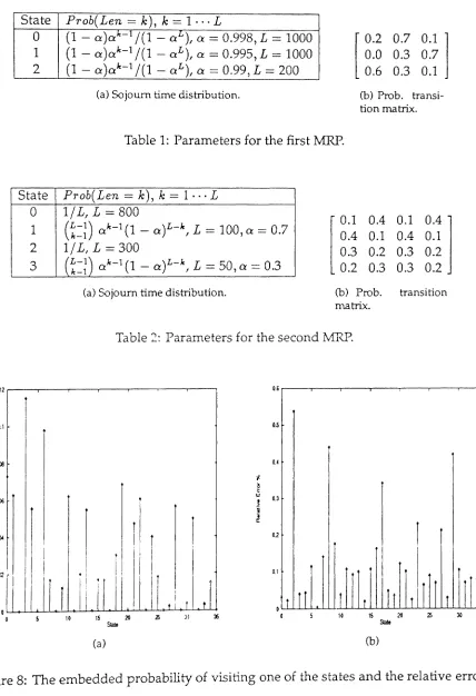
'TJ.-L2 embedded probability of visiting a particular state and the associated rela.:»e

erroris shown in figure 8, the largest erroris 0.53%. We also show the mean sojourn time

in states of the superposition and the associated relative error in figure 9. The largest

relative error is approximately 5.7%. The results in figure 10 show the distribution of

sojourn time between two arbitrary source-destination pairs. The first pair is [(1,1),(1,0)]

and [(1,0),(2,1)], while the second pair is [(0,0),(0,1)] and [(2,1)/(0/0)]. The analytic and

simulation results are almost identical.

The approximation model was observed, in general, to be accurate. We have

experi-mented with other types of distributions and different processes and found the accuracy

to bereasonable. Also, we observed that the more the states' sojourn time distribution

re-sembles a mernor vless distributions, the better the approximation is. This isdueto the fact

thatif all the sojourn time distributions are memoryless the approximate superposition is

State Prob(Len

==

k), k

==

1 ...L

0 _(1- a)a.l.:-1/ (1 - 0:£),a

==

0.998,L

==

1000

1 (1 - a)ak- 1/(1 - o:L),a

==

0.995, L

==

1000

2 (1 - a)ak-1/(1 - aL) , a

==

0.99, L

==

200

[

0.2 0.7 0.1]

0.0 0.3 0.7

0.6 0.3 0.1

(a) Sojourn time distribution. (b) Prob. transi-tion matrix.

Table 1: Parameters for the first MRP.

State Prob(Len

==

k), k

==

1 ... L

0 I/L, L == 800

1 (~=D ci-1(1 - a)L-k, L

=

100,a

=

0.7

2 1/ L, L

==

300

3

(~=D

a k-1(1 - a)L-k, L

=

50,a

=

0.3

(a) Sojourn time distribution.

0.1

0.4

0.1

0.4

0.4 0.1 0.4 0.1

0.3

0.2 0.3 0.2

0.2 0.3 0.3 0.2

(b) Probe transition matrix.

Table'2: Parameters for the second MRP.

0.6 0.5 o.~ i-~ t w _0.3 ~ i

_..

cr:: 0.2 0.1 lS 20 10 • t

!

I I I I t rI

r

r

I

r

, r

I

t r

o o 0.1 0.12 o.~ o.cw o.~ (a) (b)

•

t

•

I

I

1

tiiriltl

30 1S 20

StBtt 10

o~"""""-L...L...L...L-..&...+-J-..L-..4--L-L..L..-L-LL.J~....L...-L..1...-L...-~...L....+-L.L.U o

.,.

~

w

!

i

..

cr:

35 30

25 10

o o 200

(a) (b)

Figure 9: The mean sojourn time in a state and the relative errore

..

_.,.

-,.,

01 '''~d'''''''"11~

o 10 20 jQ J)) 50 &0 70 80 00 100

l&r9~

100 200 ~ ~ 500 600 700 ~

lefYJt\

o~____'I..---'_--L_ _ _ L_ _ _ J __ _..J__~_ _

o

0.00<11

o.~

0.00:115

o0003r---r----,----r----r---.--~--- ...

0.01.»25

-,

+.

0.002 0.003

0.001

(a) ((1,1), (1,0)) -. ((1,0), (2, 1)) (b) ((0, 0), (0, 1)) -. ((2,1), (0, 0))

Figure 10: The distribution of the sojourn time between two arbitrary states.

5.2

Validation of the Statistical Multiplexer Model

In section 4 we presented a stochastic queueing model for the analysis of a finite buffer

FIFO statistical multiplexer whpse input is a MRP which can be the superposition of a

number of independent arbitraryonloff sources. We reportresults from two experiments

that have been carried out. In the two experiments the buffer size B was taken to be

40 and there was only one server (5 == 1) in the multiplexer. Inthe graphs showing the

obtained results, the curves labeled as detailed, aggregate, and simulationdemonstrate the

results obtained by characterizing the superposition process in terms of a l2-state MRP

obtained using the results from section 2.2; by characterizing the superposition process in

terms of a 3-stateMRP obtained by the iterative aggregation algorithm; and by simulation

respectively. We note here that confidence intervals for the simulation results are not

shown because they were very narrow. This is also true for the curves shown in the

remaining sections.

Exan1ple 1:In the first experiment, we let the multiplexer input be two homogeneous

onloffsources, where the on period is deterministic and the off periodishyper-geometric

with parameters given in table 3. The constant on period length is taken from the set

{28, 63, 108,167,251} providing a source throughputor {G.l, 0.2, 0.3, 004, O.S} respectively.

Figure 11 shows the results for this particular model. We again observe here the proximity

of the results obtained by simulation and detailed superposition. The results obtained by

the aggregate superposition model are less accurate.

Mean CV2\

Off period 251 1.5

I

Table 3: Parameters of off period for results in example 1.

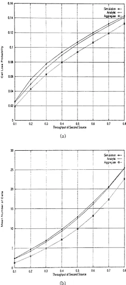
Example 2 -Heterogenous Sources: We tested the effect of source heterogeneity on the

accuracy of the queueing model by studying the case of twoheterogeneous onloffsources with hyper-geometric distribution for the on and off periods with the parameters shown

in table 4(a) and table 4(b). For the second source the mean on period

an

is adjusted such

that the source throughput takes values fromL'1eset {O.l, 0.2,0.3,0.4,0.5,0.6,0.7, O.8}. The

throughput of the first source is fixed to 0.2.

: //,

.f~/

,.:

~;

./.;-! i ..

y

1 ...

····j4~

O~

02r--I---:--t---+---+---.;.---+-~£.J

025r--r--,---r--.,---r---r---~---.

£

~ 0.15r----r----:---~--+---+--,l't-..L---L--J

.8 o

n:

.

.

o

..J

~

o

02 0.3 0.4 0.5 0.6

Uiization 0.7 0.8 0.9

(a)

I i··· ..

: . ' .~'

...~:~_-..:--~-_--.;..---o--~----J

.--':

0.5 0.6 J7

UHzalioo

0.8 0.9

(b)

Figure 11: Validation of statistical multiplexer model. Buffer Size = 40, two input on/off

sources with deterministic on and hyper-geometric off periods. (a) Cell loss probability,

0.16 r---r---r----r---~--.,r---..---Srn~a.licrl -+-~Y':-+­ AW~·8-0.12 ~---.;.----.:..---~//""""'j

/ : ... I

/

.,

.., ~

0.1r---T---:----+-~;.L_+-+---i---+----l

"i

o O.t))r---:-~~~--+---t---t---+---l

?'

~

~

e

~ o.~ r---r---r7~~~---1--~---4---J

.

o

..J

/~/

...-/1 .. "_~/

0.8

0.7 0.3 o.~ 0.5 0.6

Tht0J9~eXSocood~

02

O --""_ _--'--_ _...-_-...L_ _--L._ _..J..._----l

0.1

(a)

Srn~aba1

-+-Wytic~ Atr;e-;ate '8-2) .! "i o '0 ~ 15 E :J Z C l'll 0 ~ 10

2S1 - - - -_{: i} ---~---..I{_.

i

!

---/7r=--····_···_"'-,·

- + - --l---~

. >

~~~

•• ( . / ,

0.8

0.7 0.3 o.~ 0.5 0.6

fu0J9~ri Second So.1rD3

02

o\---_---.l.--~_-...Io..---~-_..oI_-~---..j 0.1

(b)

Figure 12: Validation of statistical multiplexer model. Buffer Size=40, two heterogeneous

detailed model and simulation results are pretty close, while the aggregate superposition

model is less accurate. The results are shown in figure 12. In example 1 the aggregate

model provided higher values than simulation, whereas in this case, it provides values

that are lower than simulation. It is not clear which parameters of the input sources

make the aggregation model give higher or lower values than the simulation results. We

observed the same behavior in the case of more than two input sources, discussed in

section 5.3.

Mean CV2

On period 62.5000 5.0

Offperiod 250 1.5

(a) Firs t source parameters

Mean CV2 On period 011, _5.0

Offperiod 250 1.5

(b)Second source parameters

Table 4: Parameters for example 2.

5.3

Valid ation of the Iterative Aggregation Algorithm

In sec:i~Jn3.2, we introduced an iterative algorithm based on the notion of aggregation to characterize the superposition process of N ~ 2arbitrary orr/off source. We study the accuracy of this algorithmbyexamining the following three examples.

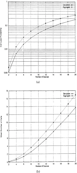
Example 1: We consider a finite buffer multiplexer with buffer size equal to 40 and one

server. All input sources are homogeneous and the on and off periods are hyper-geometric

with parameters shown in table 5. The throughput ofa single source is equal to 0.0385.

The number of input sources was increased from 2 to 20. The simualtion and analytic

results for the cell loss probability and the mean number of cells in the multiplexer queue

are shown in figure 13.

iV-lean CV2 On period 10.0 5.0

Off period 250.0 1.5

Table 5: Parameters of on and off periods.

These results indicate that the aggregation method does not have a good accuracy.

results. For this particular example, the iterative aggregation method seems to smooth

out the original superposition process bymaking it less bursty and less correlated. This

effect is magnified as the number of sources increases, because of the errors introduced

at each stage of the aggregation method. The aggregate superposition, however, still

captures the first order characteristics of the real superposition process and hence the

multiplexer witnesses a longer queue buildup and a larger cell loss probability as the

number of sources increases.

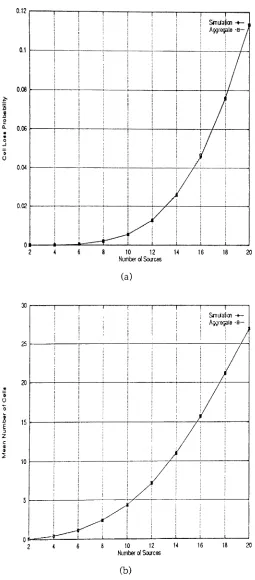
Example2:We consider the same multiplexer parameters and we let the

ani

off source

have a deterministic on period with length equal to 50 and a geometric off period with

mean equal to 1101.484. The throughput ofasingle sourceisequal to 0.0434. The number

of input sources was increased from2to20. The simualtion and analytic results are shown

in figure 14. We observe a similarbehavior as in the first example. However, in this case

the analytic results are doser to the simulation data than in the first example and they

provide

an upper

bound of the cell loss probability and the

mean

number of cells.

Exam.pIe 3:Weconsider a finite buffer multiplexer with buffer size equal to 60 and one

server. PJlinput sources are homogeneous and the on and off periods are geometric with

means11.77and2:3.23respectively. The throughput of a single sourceisequal to0.05. The

number of input sources was increased from 2 to 20. The results are shownin figure 15.

We note that the aggregation method is accurate in the case of Interrupted Bernoulli

Processes. We can then conclude that the inaccuracy in the previous cases is not due to

the successive iterations but mainly due to the aggregation process which distorts the

statistical characteristics of the original superposition process. Inthe case of heterogenous

IBP'5, the accuracy of the aggregation is acceptable if the ratio of maximum to minimum

squared coefficient of variation of the inter-arrival time is small, as demonstrated in [3].

6

Studv of

.,;

the Effect of Traffic Parameters on Queueing

Per-formance

In this section, we conduct a study of the effect of various traffic parameters on the

_. ..

-: Agg'~ -~

I

i ;_i i_I

i _i

1----I i

,

, ~ ~ .----: : ; I

: l ...

-.

,

~~.

..' : :

/: I . i - » :~ I : : : :

/ i .>:.(1. i i I

/ .tr··· _{! ! !} j !

./

.... j _i I i

I i

i

0.001 i I ! i j

: 1 : : : I

:

j : :

: :

! !

i ! \

i

:

I

!

I _{i i i}

O.COOl

2 10 12 1. 16 18 20

NumOOfclSxrces (a) 20 18 16

!

.~

,

10 12

NumCe" cJSxrces 12r l ---r----r--r-~----,.----,r---...--.,...---.! "i o '0

!

E :J Z c

"

~ ~ (b)

Figure 13: Validation of the iterative method. Buffer Size=40. All sources are identical and

have a hyper-geometric distribution for the on and off periods. (a) Cell loss probability, (b) Mean number of cells.

0.1 ~

s

~ 0 Il:

..

0 .J "i o 0.01

...

_.l-···_··t·_~

I / .

! /

/ " -I· " / ; : : ; : :

: I : :

: : /

"ll

i i i

, t

Sinuaioo

-+-A~r~~.•

?.:

Rt' ,': ...• 1

::I

1~ 12 .! ~ o '0 10

2

E :l Z C a:! ~ :i ..,~ i f.···· 20 18 16 10 12 14

NUffiOOfciSxrces

o~_~_--..L--_--..&..._--"'---"'----_.-.-_-"--_.-...._---l

2

(b)

Figure 14: Validation of the iterative method. Buffer Size = 40. All sources are identical

with a deterministic on period and a hyper-geometric off period. (a) Cell loss probability,

20

18

16

10 12 14

NumwolSxrces

y

y

~

!: !I l

: i .

j i !

.

:

: ! l ocs ~ :8 ] 0 n: 0.00

·

·

0 ..J i o 0.04 0.12 r--~-.,---.---,---,--~----.---(a) 18 16

10 12 14

NumbefdSxrces I 1 , _! , SrnLiaboo -+-A9J(EIjOlle

-8-I

Y

V

y

/

:

rr:

I :

i

:

I

i l l

:

---' o 2 20 15 10

·

i o o Z E ::l Z c as Q :l (b)

Figure 15: Validation of the iterative method. Buffer Size

=

60. All sources are identical

with a geometric on and off periods. (a) Cell loss probability, (b) Mean number of cells.

6.1

Effect of the Distribution of the On and Off Periods on the

Multi-plexer's

Pe.rforrnarice

In this section, we study the effect of the distribution of the on and off periods on the

multiplexer's behavior. In the literature, it is common to approximate the distribution of

sojourn times in a stateby a geometric or a hyper-geometric distribution. The geometric

distribution characterization requires only the first moment, while the hyper-geometric

distribution characterization requires the first two moments. The question that usually

arises is whether these approximations are accurate. We consider an extreme case where

the original input source is correlated and then study how the multiplexer's performance

would change if the source is replaced by an IBP (sojorun times are geometric) or by

a source with hyper-geometric on and off periods. Note that in these two models the

inter-arrival times are uncorrelated. We consider a single server multiplexer with two

homogeneous input sources and abuffer size taken from the set{l O, 20, 30,40,50,60}.

The distribution of the on and off periods of the original input source is a mixture of

tvo deterministic distributions. The inter-arrival time lag-1 correlation is equal to 0.048.

The parameters of the pdf of the on and off periods are shown in table 6. The throughput

of a single source is equal to 0.296, the mean on and mean off periods are 50 and 119

respectively, and the CV~ and the C~2ff are 2.332 and 13.150 respectively. Given these

values we can approximate the original source by an IBP source and a source with a

hyper-geometric on and hyper-geometric off periods.

On period Offperiod

Length Prob. Length Prob.

1 0.708333 20 0.95

169 0.291667 2000 0.05

Table 6: Parameters of the pdf of the on and off periods.

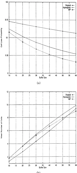
In figure 16 we plot the mean number of cells and cell loss probability for the

orig-inal source, the single-moment approximation by an IBP source, and the two-moment

approximation by a source with the hyper-geomtric on and off periods. The IEP model

underestimates the cell loss probability and overestimates themean number ofcells

(ex-cept when the buffer size increases above 52). This suggests that the rBPisnot a faithful

Sohraby [8] introduced a model for handling general on/off sources. The model

gives an approximate upper bound for the cell loss probabilityasa function of the first

two moments of the on and off periods assuming multiplexer with an infinite buffer

size. This suggests that only the first two moments of the one an off periods affect the

performance. However, the results in figure 16, demonstrate the inaccuracy of the

two-moment approximation when the buffer sizeisfmite. The approximate source model with

two-moments matching provides an underestimationofthecellloss probabilityandmean

number of cells. This shows that the two-moment approximation may not be accurate in all cases.

6.2

Effect of the Interrival-time Correlation of Traffic Sources on the

Mul-tiplexer's Performance

For an arbitrary onloffsource, the lag-l correlation coefficient of the inter-arrival timeis

gi\renby Calmes[4]:

fI

=

1on(1) -

~

1

+

C~2jf - ~

where

f

on(l) is the probability that the on periodis of length 1,

on

is the mean on period,

and

CV;}f

f is the squared coefficient of variation of the off period length. We have been

able to identify some distributions for which the value of ¢>l is non-negligible. The key

to obtaining such distributions is to concentrate a large portion of the probability mass at

length 1 of the on period distribution, i.e. make

fon(l)

as large as possible while satisfying

some of the other source characteristics (e.g. given values of

on

and/or CV~.) One

such distribution is the

mixture of two deterministic distributions

whichisa distribution that

can be of length L₁ or ~ with probabilities p and 1 - p respectively. Wefix one of the

deterministic lengths to be equal to 1and let the other be of a variable length L. Given a

particularvalueof

an

and~ andtheoffperioddistribution, we canfind valuesforpand L

which would satisfy the given values ofo1l, and ¢>l using a simple enumerative algorithm.

To study the effect of the inter-arrival time correlation on the multiplexer behavior, we consider the case of two input homogeneous sources where the off period of a source

I Ori~r}aI-+­ iHyp«gocm

-+-I

I~P

'8-I

!

I

i

I

i

I

".s. ..i: i··· i

·'t··

'.

• 110"• • • •

0.1r---~--:~~---+----T---+--+--~-~----I

~

s

]

o

cl:

.

.

o

-'

~

o

·~····~····t

·_···-·L...

i i

I !

i :

j i

45 SO 55 60

l) as 40

Bufter Size 2S

15

o~_'---'~-"'_--I._--L_---I.._--..L.._--!.._-L_...J 10

(a)

12

r--~.---,r----y---r-~-~---r---..,....----.

CKi9rlaJ-+-iHypa-QOOTl

-+-; lap ·8·-I

!

10 15 25 3) as 40

Buffer Size

45 50 55 60

(b)

Figure 16: Effect of the distribution of the on and off periods on the multiplexer's

Sin~atiQ1

-+-

~ytic-+-I

0.15

E

:8 / '

~ ~/

2

Q.

.

_0.1 , /

tl

0 .J

~

o

0.05

0.45

0.4 02 0.25 0.3 0.35

Lag-l Caelation Coefficient 0.15

O'"-_--A-_ _~_ _ _ L_ ____L__ _.L..__ __L_ ___l

0.1

(a)

12

10

r _! 1 I _!

i i Sin~atio1

-+-:

i

I

r~ -+-!

!

I

_~

----!

:

o

Ql 0.15 02 0.25 0.3 0.35

Lag-I Caetltion Ccefficient

0.4 0.45

(b)

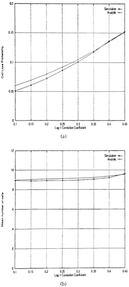
Figure 17: Effect of correlation on the multiplexer's performance. Buffer Size = 40, two

input onloffsources with hyper-geometric on and off periods. (a) Cell loss probability,

(b) Mean number of cells.

is fixed at 50, making the source's throughput equal to 0.35. Using the mixture of two

deterministic distributions for the on period, we vary

4>t

so that it takes values from the

set {O.lO, 0.15,0.20,0.25,0.30,0.35,0.40, 0.45}. The value ofp and L satisfying the given

parameters is then calculated. The cell loss probability and the mean number of cells in

the multiplexer queue are shown in figure 17.

We note that by increasing the lag-l correlation, the cell loss probability and the mean

number of cells increase. As it can be seen from figure17,the cell loss probability increases

more sharply than the mean number of cells with the increase of the correlation coefficient.

The mean number of cells is almost constant and increases very slowly with the increase

of the correlation coefficient.

6.3

Effect

of the Squared Coefficient of Variation of the on and off periods

on the Multiplexer's Performance

Using the versatile hyper-geometric distribution we studied the effect of the squared

coeffident of variation of the on and off periods, respectively CV;. and cvo~f' on the

multiplexer's performance. Byspecifying the mean and squared coefficient of variation of

the period length, itispossible to fit a hyper-geometric distribution given some conditions

are metbythe specified mean and coefficient of variation ( see [2]for more details).

We considered two input sources each with a throughput fixed at0.4. The mean on and

off periods were fixed at 100 and 150 respectively. CV;. andCVo

2

f! take values from the set

{l.O, 5.0, 10.0,15.0.20.0}. The results obtained from simulation and detailed superposition

are shown in figure 18. Note that by increasing the CV~, while CVo~f is kept constant,

both the cell loss probability and mean number of cells increase (see parts (a) and (b) of

figure 18). Also, note that the rate of increase of the mean number of cells and cell loss

probability whenCV;. E [1,5]islarger thanfor the rest of the values. Moreover, for larger

values of CV;ff' the rate of increase of cell loss probability and mean number of cells

as a function ofCV;. is relatively slower than for smaller values of

cV;J

J. A surprising

result is observed when varying C~2ffwhile CV~ is kept constant (see parts (c) and (d)

of figure 18). As CV;ffincreases, the cell loss probability

increases

while the mean number

17

-y---

_

~ orr CV2 - 1

... orr CV2 - 5

...- orr CV2 - 10

•••~•... orr CV2 - 15

... orr CV2 - 20

20 15 10 .

...

~.~ ~

...•...

~

.

.

-

..

-.,... D ••· · · - · · · ·

~./.

". o::

:::~

·

/

r:-:;.··:::::·:·_···-/ ..~P:::"~·

A/;~~~~~;::::~····

~

....

o 15

13

12-t---r----~---

...

- - - . . : I

~

o

20

--...- orr CV2 - 1

•• - .... _. OrT CV2 - 5

._..,..._. OrT CV2 - 10

•• _,;r._'OrT CV2 - 15

.•-..,..._. orr CV2 - 20

0.1'70 0.165 0.160 >. +oJ orl ~ 0.155 ~_e ~ 0.150

..

'" S 0.1.t5 ~ ~ u 0.140 0.135 0.130 0

OM CV2 OM CV2

(a) (b)

0.1& - , - - - 1&

-r---20 ····0-..·ow CV2 - 1.0

····0--· C)II CV2 - 15

.0' • .,. __ ' 0If CV2 - 20

• • • • • • • _ . ()tlI CV2 - 5

o

12-+- -....

---J

15

..

.... ...._~ tJ ~ 0 ~ ₁₄

i

:z: ~ :i 13 20

- . . . . - OM CV2 - 1 . -. . . _- OM CV2 - 5

._••• _ - OM CV2 - 1. 0

._~o---OM CV2 - 1.5

.-...,._- ow CV'2 - 20

o

O.1..t

O.1~

0.13-+--+---1

orr CV2 orr CV2

(c) (d)

Figure 18: Effectofthe squared coefficient of variation of the on and off periods on

mul-tiplexer's performance. Buffer Size

=

40, two input

ani

off sources with hyper-geometric

on and off periods. (a) Cell loss probability vs. CV;'. (b) Mean number of cells vs. CV;'.

(c) Cell loss probability vs. CV;ff' (d) Mean number of cells vs. CV;ff'

7

Conelusions

In this paper we presented a new approximation method for characterizing the

superposi-tion of multiple independent Markov Renewal Processes. The presentasuperposi-tion here focused

on discrete-time processes, but the methodology is readily applicable to continuous-time

processes with little modification. The model developed for characterizing the

superpo-sition can be directly applied to the area of tele-traffic engineering and statistical

multi-plexing. One special case of this model is the arbitrary

onl

off source that was used in this

paper. We have presented a queueing model for the analysis of a statistical multiplexer

whose inputis a :rvfRP representing the superposition of multiple traffic sources.

The advantage of our methodology is that it provides a uniform framework in which

a variety of models of traffic sources can be handled. The basic limitation is the huge state

space and the computational complexity of the algorithms. These disadvantages can be

overcomeifan elegant state aggregation scheme is found such that the resulting aggregate

process has a number of states which is preferably a linear function of the number of

sources while still preserving the characteristics of the real superposition process. We

introduced an aggregation scheme for reducing the dimensionality of the superposition

process. However, during the aggregation, the statistical properties of the original process

may be distorted and may subsequently lead to inaccurate results for the multiplexer's

performance metrics.

The work presented here introduces many challenging issues. An important problem

that is yet to beconsidered is the characterization of the departure process from a

mul-tiplexer with multiple arbitrary orr/off input sources, or in general, with an :rvfRP input.

Characterizing the departure process of one of the input sources isev~nmore challenging.

The methodology presented here introduced a new versatile modeling device for arrival

processes which can be called the Batch Semi-Markov Arrival Process (B-SMAP). This is

a semi-Markov process with as many states as necessiated by the physical source being

modeled, and in which the sojourn times in states are arbitrarily distributed. This process

is analogous to the well-known BMAP. However, it is more flexibile than a BMAP but

References

[1] W. P. CherryandR. L.Disney. The Superposition of Two Independent Markov Renewal

Processes. Zastosowania Matematyki,17:567-602, 1983.

[2] T.E. Eliazov, V. Ramaswami, W. Willinger, and G. Latouche. Performance of an ATM Switch: Simulation Study. In Proceedings of theIEEEInfocom, pages 644-659, 1990.

[3] K. M.Elsayed andH. G.Perras. AComputationally Efficient Algorithm for

Character-izing the Superposition of Multiple Heterogeneous Interrupted Bernoulli Processes. Submitted for publication, 1994.

[4] S. Calmes. Analysis of On-Off Processes With Independent Arbitrary Distributions. Unpublished technical report, North Carolina State University, 1992.

[5] J. Hunter. Mathematical Techniques of Applied Probability. Volume2: Discrete TimeModels: Techniques and Applications,chapter 9. Academic Press, 1983.

[6] V. S. Korolyuk. Superposition of Markov Renewal Processes. Cybernetics, 17:556-560, 1981.

[7] M. F. Neuts. Matrix-Geometric Solution in Stochastic Models: An Algorithmic Approach.

John Hopkins Univ. Press, 1981.

[8] K. Sohraby. On the Theory of General On-Off Sources With Applications in High-Speed Networks. In Proceedings of the IEEE Infocom, pages 401-410, 1993.