INVESTIGATION
Rapid and Robust Resampling-Based
Multiple-Testing Correction with Application
in a Genome-Wide Expression Quantitative
Trait Loci Study
Xiang Zhang,*,†,1Shunping Huang,†,1Wei Sun,‡,§and Wei Wang†,2 *Department of Electrical Engineering and Computer Science, Case Western Reserve University, Cleveland, Ohio 44106, and Departments of†Computer Science,‡Biostatistics, and§Genetics, University of North Carolina, Chapel Hill, North Carolina 27599
ABSTRACTGenome-wide expression quantitative trait loci (eQTL) studies have emerged as a powerful tool to understand the genetic basis of gene expression and complex traits. In a typical eQTL study, the huge number of genetic markers and expression traits and their complicated correlations present a challenging multiple-testing correction problem. The resampling-based test using permutation or bootstrap procedures is a standard approach to address the multiple-testing problem in eQTL studies. A brute force application of the resampling-based test to large-scale eQTL data sets is often computationally infeasible. Several computationally efficient methods have been proposed to calculate approximate resampling-basedP-values. However, these methods rely on certain assumptions about the correlation structure of the genetic markers, which may not be valid for certain studies. We propose a novel algorithm,rapid andexact multiple testing correction by resampling (REM), to address this challenge. REM calculates the exactresampling-basedP-values in a computationally efficient manner. The computational advantage of REM lies in its strategy of pruning the search space by skipping genetic markers whose upper bounds on test statistics are small. REM does not rely on any assumption about the correlation structure of the genetic markers. It can be applied to a variety of resampling-based multiple-testing correction methods including permutation and bootstrap methods. We evaluate REM on three eQTL data sets (yeast, inbred mouse, and human rare variants) and show that it achieves accurate resampling-based P-value estimation with much less computational cost than existing methods. The software is available athttp://csbio.unc.edu/eQTL.
G
ENOME-WIDE studies of expression quantitative trait loci (eQTL) have been widely used to dissect the genetic basis of gene expression and molecular mechanisms underly-ing complex traits (Bochner 2003; Rockman and Kruglyak 2006; Michaelsonet al. 2009). In a typical eQTL study, the association between each expression trait and each genetic marker [e.g., single-nucleotide polymorphism (SNP)] is as-sessed separately, which leads to a huge number of correlated tests. Appropriate multiple-testing correction is crucial for eQTL studies. The resampling-based test using permutation or bootstrap (Good 2005) has been widely used formultiple-testing correction across multiple genetic markers for each phenotype (Barrettet al.2005; Purcellet al.2007) by simu-lating the null distribution using permuted or bootstrapped phenotype values (Westfall and Young 1993; Churchill and Doerge 1994; McClurg et al. 2007). More specifically, the
phenotype values are randomly shuffled and reassigned to individuals with or without replacement (i.e., bootstrap and permutation, respectively). For each resampled phenotype a whole-genome scan is performed tofind the maximum test statistic among all SNPs. The correctedP-value is the propor-tion of the resampled phenotypes where the maximum test statistics are greater than the maximum test statistic in the original data. We refer to such a corrected P-value as the
resampling-based P-value. The resampling-based test
pre-serves the correlation structure of the SNPs and does not require any distribution assumption on the test statistic.
Another level of multiple-testing problem in eQTL studies is the multiple tests across tens of thousands of gene
Copyright © 2012 by the Genetics Society of America doi: 10.1534/genetics.111.137737
Manuscript received December 11, 2011; accepted for publication January 8, 2012 Supporting information is available online at http://www.genetics.org/content/ suppl/2012/01/31/genetics.111.137737.DC1.
1These authors contributed equally to this work.
2Corresponding author: Department of Computer Science, University of North Carolina,
expression traits (Kendziorski and Wang 2006). One standard solution isfirst to estimate the resampling-basedP-value (of the most significant association) for each expression trait and then to determine a threshold for the corrected P-values across all expression traits by controlling the false discovery rate (FDR) (Benjamini and Hochberg 1995; Storey 2003).
Although this approach is ideal for eQTL studies, its intensive computational burden has greatly limited its practical use. For example, supposing that a corrected P -value threshold of 0.01 is needed to control the FDR, up to 100,000 permutations/bootstraps may be needed to esti-mate such a resampling-based P-value accurately. Consider a typical scenario where there are 500,000 SNPs and 20,000 expression traits. The total number of tests is 500,000 · 20,000 · 100,000 = 1015. A brute force implementation of the resampling-based test is clearly not practical. Compu-tationally efficient methods are highly desirable.
To tackle the computational challenge, several methods have been proposed to approximate the resampling-basedP -values. One approach is to estimate the effective number of independent tests from the eigenvalues of the correlation matrix of the SNPs (Cheverud 2001; Nyholt 2004; Li and Ji 2005; Gaoet al.2008; Moskvina and Schmidt 2008; Pe’er
et al.2008). Previous studies have shown that these meth-ods may yield inaccurate results (Salyakinaet al.2005; Han
et al. 2009). Another approach, relying on the assumption
that the test statistics over multiple SNPs asymptotically follow a multivariate normal distribution (MVN), calculates the permutation P-values by directly sampling from the MVN distribution (Lin 2005; Seaman and Müller-Myhsok 2005; Conneely and Boehnke 2007; Hanet al.2009). Both the“effective number of independent tests”and MVN meth-ods cannot be directly applied to genome-wide association studies when the number of SNPs is much larger than the sample size. A common strategy is to divide all the SNPs into contiguous blocks, to apply these two methods to each block of SNPs, and then to combine the results across the SNP blocks. This partition–ligation approach implicitly assumes that the SNPs between two blocks are weakly correlated. From a different perspective, an approximation method based on a geometric interpretation of permutationP-values has been proposed in Sun and Wright (2010). This method does not require any asymptotic distribution of the test sta-tistics, but it assumes a Markov type of dependency among the markers. Another method has been developed to correct very significant P-values in disease association studies by importance sampling (Kimmel and Shamir 2006). This method is designed for binary phenotypes and cannot be directly applied to quantitative expression traits.
Despite the success of the aforementioned approximation methods, their accuracies rely on the validity of the following assumption: the nearby SNPs are correlated whereas the distant SNPs are not. This assumption may not be valid. Please refer to supporting information, File S1 for further discussion on the assumptions of the existing approximation methods.
For the resampling-based test, the total computational time is equal to the average time needed to calculate each test statistic multiplied by the total number of tests. Several algorithms have been developed to speed up the exhaustive resampling-based test by calculating each test statistic more efficiently. For example, if the phenotype is binary, compu-tational efficiency can be improved by efficient computation of contingency tables (Browning 2008) or by bit arithmetic operations (Pahl and Schafer 2010). For eQTL studies, a summation tree can be utilized to compute the test statis-tics incrementally (Gattiet al.2009). Note that these meth-ods are specifically designed for permutation tests and are not applicable to bootstrapping. In this article we tackle the computational challenge of the exhaustive resampling-based test from another perspective. That is, we try to reduce the number of test statistics that need to be calculated. We pres-ent an algorithm,rapid andexactmultiple testing correction by resampling (REM), which prunes the search space and performs tests only on a small proportion of the SNPs. This is achieved by constructing a two-layer indexing structure that groups SNPs on the basis of their genotypes. The SNPs in one group share a common upper bound on the test statis-tics. Actual tests are performed only in the groups whose upper bounds are greater than a certain threshold. REM is
guaranteed to find the exact resampling-based P-values. It can be applied to a variety of resampling-based methods, including permutation (Westfall and Young 1993; Churchill and Doerge 1994) and bootstrap (McClurget al.2007). We evaluate the performance of REM on yeast segregants, mouse inbred strains, and human rare variants data. The results demonstrate that REM not only returns the exact resampling-based P-values, but also runs orders of magni-tude faster than alternative methods.
Materials and Methods
Problem formulation
We consider binary genotype data. The binary genotype may appear in haploid organisms, such as yeast, inbred diploid organisms, such as inbred mice, or rare variants where the genotype of a homozygous rare allele is unlikely to occur and is collapsed with a heterozygous genotype if it does occur. Without loss of generality, we denote the common and rare genotypes by 0 and 1, respectively.
The permutation test based on the maximum test statistic across all SNPs was originally described in Westfall and Young (1993) and applied to a genome scan in Churchill and Doerge (1994). This approach preserves the correlation structure of the SNPs and requires a much smaller number of permutations than the procedures that first compute point-wise P-values and then apply adjustments (Nettleton and Doerge 2000). The weighted bootstrap approach (McClurg
Let {X1,. . .,XN} be the SNPs and {Y1,. . .,YM} be the gene expression traits. Let T(Xn, Ym) denote the test statistic be-tweenXn(1#n#N) andYm(1#m#M). LetTYmbe the maximum test statistic forYm. Suppose that we resample the phenotype K times. For a resampled phenotypeYk
m, we de-note its maximum test statistic asTYk
m. Fork= 1,. . .,K, let
Ak¼
(
1 if TYm,TYmk 0 if TYm$TYmk:
The resampling-basedP-value ofYmis defined as
PresðYmÞ ¼
PK
k¼1Akþ1
Kþ1 :
To calculate the resampling-based P-value of expression traitYm, thecomputational problemis to determine, for every
Yk
mð1# k #KÞ, whether its maximum test statistic TYk m is larger thanTYm. A brute force solution to this problem is that, for everyYm;k we perform a complete scan of all SNPs tofind the maximum test statistic and compare it to TYm. This ap-proach has been adopted in most existing exhaustive methods that calculate the exact resampling-basedP-values. Next, we discuss how our algorithm, REM, can efficiently compute the solution without calculating the test statistics for all SNPs. General idea of the proposed method
The key idea of the proposed algorithm is as follows. We partition SNPs into different groups on the basis of their allele frequencies. For each group of SNPs, we can find an upper bound on the test statistics. If the upper bound is lower than a certain threshold, there is no need to calculate the test statistics for this group of SNPs. The actual tests are performed only for the groups of SNPs whose upper bounds are larger than the threshold.
The groups of SNPs are organized into a two-layer indexing structure. Utilizing indexing structures for efficient computation has been a longstanding research focus of the database management and theoretical computation research communities. The idea of indexing SNPs and exploring the upper bound on test statistics was originally investigated in epistasis detection in a genome-wide association study (Zhanget al.2009, 2010). In this article we apply this gen-eral methodology to the problem of multiple-testing correc-tion in eQTL studies.
Next wefirst introduce the two-layer indexing structure that groups SNPs on the basis of allele frequencies. Then we discuss how to use this indexing structure to obtain the upper bound on the test statistics for each group of SNPs and thus dramatically reduce the number of test statistics to be calculated.
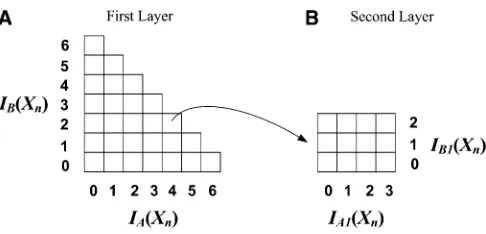
The indexing structure
First layer:Suppose that there areSindividuals {I1,I2,. . .,IS} in the study. We partition the individuals into two subsets:IA= {I1, I2,. . .,I⌊S/2⌋} and IB = {I⌊S/2⌋+1, I⌊S/2⌋+2,. . .,IS}. Note
that the partition of individuals is random and only done once for the entire data set.
For a SNPXn, we use |IA(Xn)| and |IB(Xn)| to denote the numbers of rarer genotype (i.e., the number of 1’s) in par-titions IA and IB, respectively. We can group the SNPs by their (|IA(Xn)|, |IB(Xn)|) values and index them in a two-dimensional (2D) array. The SNPs with the same (|IA(Xn)|, |IB(Xn)|) values will fall into the same entry in the array.
For example, suppose that there areS= 12 individuals in our study. We can partition them into two subsets, each having 6 individuals. Figure 1A shows thefirst layer of the 2D index-ing structure. The SNPs havindex-ing the same (|IA(Xn)|, |IB(Xn)|) value fall into the same entry in the 2D array. In this example, the possible values of |IA(Xn)| and |IB(Xn)| are {0, 1, 2,. . ., 6}. Recall that 1 denotes the rarer genotype, and thus the number of 1’s in any SNP is no greater than
⌊
S/2⌋
; i.e., |IA(Xn)| + |IB(Xn)|#⌊
S/2⌋
. Therefore, the indexing struc-ture has entries only below the diagonal, as shown in Figure 1A. Later we show that the SNPs in the same entry [i.e., with the same (|IA(Xn)|, |IB(Xn)|) value] share a common upper bound on their test statistics.Second layer:Applying a similar idea, we can build a second layer indexing structure for each entry in thefirst layer. For a group of SNPs in the same entry in the first layer, we further partition individuals inIAinto two subsets:IA1= {I1,
I2,. . .,I⌊S/4⌋} andIA2= {I⌊S/4⌋+1,I⌊S/4⌋+2,. . .,I⌊S/2⌋}. Sim-ilarly, we partition IBinto two subsetsIB1andIB2of similar sizes. Note that these partitions are random and done only once for the entire data set. For any SNPXn, we use |IA1(Xn)|, |IA2(Xn)|, |IB1(Xn)|, and |IB2(Xn)| to denote the number of 1’s ofXninIA1,IA2,IB1, andIB2, respectively. The group of SNPs in the same entry in the first layer is further partitioned by its (|IA1(Xn)|, |IB1(Xn)|) values. The SNPs with the same (|IA1(Xn)|, |IB1(Xn)|) values fall in the same entry in the second layer indexing structure.
Following the previous example where there are 12 individuals, its first layer indexing structure is shown in Figure 1A. For a particular first layer entry (|IA(Xn)|, |IB(Xn)|) = (4, 2), its second layer indexing structure is shown in Figure 1B. It is easy to see that the maximum value that |IA1(Xn)| can take is min{|IA(Xn)|,
⌊
S/4⌋
}, and themaximum value that |IB1(Xn)| can take is min{|IB(Xn)|,
⌈
S/4⌉
}. This is reflected in the following example: the maximum value of |IA1(Xn)| is min{4, 3} = 3, and the maximum value of |IB1(Xn)| is min{2, 3} = 2.Similar to thefirst layer, the SNPs in the same entry in the second layer also share a common upper bound on their test statistics. We will show that this bound is tighter than (or at least as tight as) the bound derived from thefirst layer.
Upper bound on the test statistics
In this subsection, we give a common upper bound on the test statistics for the SNPs in the same entry in the indexing structure. An intuitive explanation is as follows. For SNPXnand a resampled phenotype Yk
m, letY1 represent the sum of the phenotype values of the individuals with rarer genotypes (i.e., whenXn= 1). It can be shown that many statistics are convex functions ofY1(seeFile S1for details). If we can determine the range ofY1, we can easily derive an upper bound of the statis-tics. It can be shown that the SNPs in the same entry have the same range forY1 and hence share a common upper bound.
Next, wefirst discuss how to obtain the upper bound for a SNP group in thefirst layer, and then we show that tighter bounds can be achieved for the groups in the second layer.
First layer:Recall that when building thefirst layer index-ing structure, we partition the individuals into two subsets,
IAandIB. The indexing structure groups SNPs on the basis of their (|IA(Xn)|, |IB(Xn)|) values,i.e., the numbers of rarer genotypes in the two subsets of individuals. For a resampled phenotype vectorYk
m, we useYmkðIAÞ ¼ fy1k;y2k; . . .; yk⌊S=2⌋g and Yk
mðIBÞ ¼ fyk⌊S=2⌋þ1;y⌊kS=2⌋þ2; . . .; ykSg to denote the phenotype values of the individuals inIAandIB, respectively.
Letyk
Að1Þ#yAkð2Þ#⋯#ykAðjIAjÞrepresent the ordered phenotype values in Yk
mðIAÞ and ykBð1Þ#yBkð2Þ#⋯#ykBðjIBjÞ represent the ordered values inYk
mðIBÞ. ForanySNPXnin thefirst layer entry (|IA(Xn)|, |IB(Xn)|), we have that
XjIAðXnÞj i¼1 y
k AðiÞþ
XjIBðXnÞj i¼1 y
k BðiÞ
|fflfflfflfflfflfflfflfflfflfflfflfflfflfflfflfflfflfflfflfflfflfflfflfflfflffl{zfflfflfflfflfflfflfflfflfflfflfflfflfflfflfflfflfflfflfflfflfflfflfflfflfflffl}
RL
#Y1; (1)
wherePjIAðXnÞj
i¼1 yAðiÞ is the sum of the smallest |IA(Xn)| phe-notype values of individuals inIA, and
PjIAðXnÞj
i¼1 yBðiÞis the sum of the smallest |IB(Xn)| phenotype values of individuals inIB. Recall that |IA(Xn)| + |IB(Xn)| is equal to the number of rarer genotypes and Y1 is the sum of the phenotype values of individuals with rarer alleles. Clearly, the inequality holds. We useRLto represent the left-hand side of inequality (1).
Similarly we have that
Y1#XjiI¼jAjI
Aj2jIAðXnÞjþ1y k AðiÞþ
XjIBj
i¼jIBj2jIBðXnÞjþ1y k BðiÞ
|fflfflfflfflfflfflfflfflfflfflfflfflfflfflfflfflfflfflfflfflfflfflfflfflfflfflfflfflfflfflfflfflfflfflfflfflfflfflfflfflfflffl{zfflfflfflfflfflfflfflfflfflfflfflfflfflfflfflfflfflfflfflfflfflfflfflfflfflfflfflfflfflfflfflfflfflfflfflfflfflfflfflfflfflffl}
RU
: (2)
We useRUto represent the right-hand side of inequality (2). For a given resampled phenotype vectorYk
m, inequalities (1) and (2) give us the range ofY1. That is, for any SNPXnin
the entry (|IA(Xn)|, |IB(Xn)|) of the first layer indexing structure, we have thatY1 2 ½RL;RU.
The maximum value of any convex function is attained at the boundary of its convex domain (Boyd and Vandenberghe 2004). Therefore, for the SNPs in the entry (|IA(Xn)|, |IB(Xn)|), the upper bound on test statistics is attained whenY1¼RL or
Y1¼RU.
Second layer:Similarly, we can obtain an upper bound on the test statistics for the SNPs in an entry of the second layer. We partition the values in the resampled phenotype vector
Yk
m into four groups, each across individuals in IA1, IA2, IB1, andIB2,respectively. LetfY
k A1ðiÞg;fy
k A2ðiÞg,fy
k
B1ðiÞg, andfy
k B2ðiÞg
represent the ordered phenotype values in the four groups. We have the following two inequalities:
XjIA1ðXnÞj i¼1 y
k A1ðiÞþ
XjIA2ðXnÞj i¼1 y
k A2ðiÞþ
XjIB1ðXnÞj i¼1 y
k B1ðiÞþ
XjIB2ðXnÞj i¼1 y
k B2ðiÞ |fflfflfflfflfflfflfflfflfflfflfflfflfflfflfflfflfflfflfflfflfflfflfflfflfflfflfflfflfflfflfflfflfflfflfflfflfflfflfflfflfflfflfflfflfflfflfflfflfflfflfflfflfflfflfflfflfflfflfflfflfflfflfflfflfflfflffl{zfflfflfflfflfflfflfflfflfflfflfflfflfflfflfflfflfflfflfflfflfflfflfflfflfflfflfflfflfflfflfflfflfflfflfflfflfflfflfflfflfflfflfflfflfflfflfflfflfflfflfflfflfflfflfflfflfflfflfflfflfflfflfflfflfflfflffl}
R9L
#Y1;
(3)
Y1# P
jIA1j
i¼jIA1j2jIA1ðXnÞjþ1
ykA1ðiÞþ P
jIA2j
i¼jIA2j2jIA2ðXnÞjþ1
ykA2ðiÞ
þ jP
IB1j
i¼jIB1j2jIB1ðXnÞjþ1
yk B1ðiÞþ
P
jIB2j
i¼jIB2j2jIB2ðXnÞjþ1
yk B2ðiÞ:
(4)
LettingR9LðR9UÞbe the left (right)-hand side of inequality (3) [inequality (4)], thenY12 ½R9L;R9U. The upper bound on the test statistics is attained whenY1¼R9LorY1¼R9U. It is easy to show that RL#R9L and R9U#RU. Therefore, we can get a tighter (or at least an equally tight) upper bound by uti-lizing the second layer indexing.
The REM algorithm
Given the SNPs and gene expression traits, REM returns the significant traits whose resampling-based P-values are no greater than a user-specified thresholdPt. IfPt= 1, REM returns the resampling-based P-values for all expression traits. The number of permutations/bootstraps is an input parameter provided by the user. The pseudocode of the al-gorithm is outlined inFile S1.
For every phenotypeYm, REMfirst scans all SNPs tofind the maximum statistic TYm. Then REM calculates a variable
count, which records the number of resampled phenotypes
whose maximum test statistics are greater thanTYm, as fol-lows. For each Yk
m, REMfirst checks the entries in the first layer of the indexing structure. It goes to the second layer only if the upper bound of afirst layer entry is greater than
TYm. If the upper bound of the second layer entry is still greater thanTYm, REM will perform actual tests on the SNPs in the second layer entry; otherwise this group of SNPs will be skipped because their test statistics are guaranteed to be no greater thanTYm.
for a resampled phenotype vectorYk
m, as long as wefind any SNP whose test statistic is greater than TYm;we know its maximum test statistic TYk
m will also be greater than TYm: Therefore, there is no need to scan the remaining SNPs. The other pruning strategy is based on the significance threshold
Pt. For an expression traitYm, once we have already exam-ined enough resampled phenotype vectors such that its cor-rectedP-value is greater thanPt, there is no need to examine the remaining resampled phenotype vectors. The detailed analysis of the time complexity of REM is given inFile S1.
REM can be applied to various resampling methods. For example, in addition to the permutation and bootstrap methods (Westfall and Young 1993; Churchill and Doerge 1994; McClurg et al. 2007) that preserve the correlation structure of SNPs, a resampling method that preserves the correlation structure of the expression data was proposed in Breitling et al.(2008). When generating resampled pheno-type vectors, this approach permutes the individual labels so that each individual is assigned the genotype of another random individual, while the expression profile of this in-dividual is unchanged. When the mapping is repeated on these permuted data, the correlation structure of gene ex-pression is maintained. These methods differ in how they generate the resampled phenotype vectors,i.e., line 4 inFile S1, Algorithm S1. REM willfind the exact resampling-based
P-values for the resampling method adopted by the user. Note that REM can be easily modified to identify multiple SNPs that are significantly associated with a gene expression trait. One naive approach is to apply REM to each of the top
T SNPs that are significantly associated with the gene
ex-pression trait. Since we compare the test statistic of thet-th most significant association with the maximum test statistics from the resampled data, the estimate of the resampling-basedP-value is conservative. However, as long asTis much smaller than the total number of SNPs, the bias of the esti-mate is small. A drawback of this naive approach is the computational burden increases linearly withT. An alterna-tive, and more sophisticated approach is to directly calculate the desired percentile of the maximum test statistic. For example, suppose that the desired significance level isa= 0.05, and thus we aim to estimate the 95th percentile of the maximum test statistic from 1000 permutations/bootstraps. In other words, we want tofind the 50th largest maximum test statistics among the 1000 maximum test statistics. We
can first carry out 50 permutations/bootstraps and record
the corresponding 50 maximum test statistics without prun-ing. Then we carry out the following permutation/boot-straps with pruning by keeping track of the largest 50 maximum test statistics and using the value of the 50th one as the threshold for pruning.
Results
We evaluate the accuracy and computational efficiency of REM and several representative existing methods. For approximation methods, we choose SimpleM (Gao et al.
2008) to represent the approaches of estimating the number of independent tests, and SLIDE (Hanet al.2009) to repre-sent the approaches using the MVN framework. These two methods have been shown to be superior to other alterna-tives within their classes. We also study the performance of the method in Sun and Wright (2010), which we call GeoP. For exhaustive methods, we study the performance of PLINK (Purcell et al.2007) and FastMap (Gattiet al.2009). Note that these two methods are designed to speed up only per-mutation test but not bootstrapping. Other approaches, such as the approximation method RAT (Kimmel and Shamir 2006) and exhaustive methods PRESTO (Browning 2008) and PERMORY (Pahl and Schafer 2010), are applicable only to binary phenotypes and therefore are not applicable to eQTL mapping. We evaluate the performance of the selected methods on three eQTL data sets: inbred mouse strains, yeast segregants, and human rare variants.
Inbred mouse strains
We use the hypothalamus eQTL data of inbred mice from McClurg et al.(2007). There are 32 mouse strains in the data set. The total number of SNPs is 156,525. The missing values are imputed by the algorithm in Robertset al.(2007). There are 36,182 probes on the gene expression array. Here we refer to the gene expression captured by each probe as an expression trait. Following the samefiltering method as in Gattiet al.(2009), we dropped any expression trait whose expression values are all,200 or whose largest difference in expression across the 32 mouse strains is less than three-fold. There are 3,672 expression traits left afterfiltering.
Accuracy evaluation: Due to the population structure of these inbred mouse strains, some strains are more similar to each other than other strains, and thus a direct application of a permutation test is not appropriate (Fei et al. 2006; McClurget al.2007; Churchill and Doerge 2008). We adopt the weighted bootstrap approach proposed by McClurget al.
of resamplings to be 1 million for SLIDE. The number of resamplings is also set to be 1 million for GeoP. SimpleM is not a resampling-based method and we use its default setting. Following a similar approach as in Han et al.
(2009; Pahl and Schafer 2010), we construct a 95% confi-dence interval to cover the sampling error of REM.
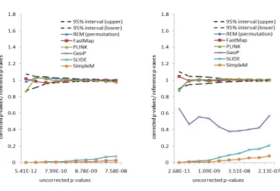
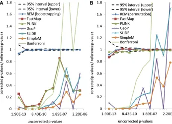
Figure 2A depicts the ratios between the correctedP -val-ues and the reference P-values for the selected methods. A method is accurate if its ratio is close to 1. As shown in Figure 2A, there is discrepancy between the bootstrap and the permutation test (as implemented in PLINK and Fast-Map). This reflects the effect of the population structure of the inbred mouse strains. The permutation test is anticon-servative compared to the weighted bootstrap method. The approximation methods, which are designed to estimate the permutation P-values, are shown to be anticonservative compared to both the bootstrapping and the permutation test. This indicates that these approximation methods are not replacements for exhaustive permutation tests. The cor-rectedP-values from the widely used Bonferroni correction are also shown in Figure 2A. It can be seen that the Bonfer-roni correction can be either conservative or anticonserva-tive for different uncorrectedP-values. Thus it is not an ideal approach for multiple-testing correction in eQTL studies.
For comparison purposes, in addition to the weighted bootstrap method, we also apply the permutation test using REM. The basic experimental setting is similar to that in the weighted bootstrap method. We estimate the reference permutationP-values of the 10 expression traits by 100 mil-lion permutations. The reference permutation P-values range from 0.00018 to 0.053. For the three exact methods, REM, FastMap, and PLINK, we use 1 million permutations to estimate the correctedP-values.
Figure 2B shows the ratio between the correctedP-values and the reference permutation P-values. The corrected P -values generated by the three exact methods fall in the confidence region of the reference P-values. In contrast, the three approximation methods, GeoP, SLIDE, and Sim-pleM, do not estimate the permutation P-values accurately. Thus these approximation methods cannot replace the exact permutation test. Further comparison between the exhaus-tive permutation test and the approximation methods will be conducted in yeast segregants and human rare variants data.
Using the genotype data of these 32 mouse inbred strains, we also study the accuracy of the selected methods for three synthetic phenotypes whose values follow standard normal, exponential, and uniform distributions. The approx-imation methods are shown to be anticonservative. Please see File S1for further details.
Computational efficiency evaluation: We evaluate the computational efficiency of the three selected exact resam-pling methods, REM, FastMap, and PLINK. The approxima-tion methods are usually very fast but do not provide accurateP-value correction. They are not considered in the computational efficiency evaluation. All experiments in this subsection are performed on a single CPU of a 2.6-GHz PC with 8 G memory running the Linux operating system.
Table 1 shows the runtime of the three methods when applied to the entire eQTL data set with 3600 phenotypes. As can be seen, with 100,000 resamplings, REM canfinish within 1 day if we set the threshold to be 1. If wefind only the expression traits that have significant associations, REM
canfinish within a few hours. FastMap and PLINK will take
a much longer time.
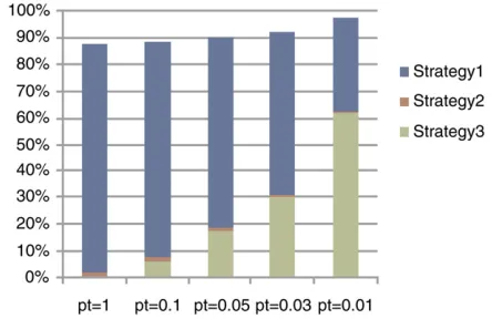
Figure 3 shows the percentage of the SNPs that are pruned by REM under different significance levels. The pruned SNPs are the ones on which we do not perform any test. If we calculate the corrected P-values for all expression traits,
.80% of SNPs are pruned. In most cases, we are interested only in the traits whose correctedP-values are less than a cer-tain threshold. At a significance level of 0.01,.97% of SNPs are pruned, which means that we need to calculate test sta-tistics only for ,3% of SNPs. This dramatically reduced search space explains the improved computational efficiency of REM. Recall that REM has three pruning strategies to re-duce the search space. They are (1) pruning by the upper bound, (2) pruning by the maximum statistic (lines 13–16 inFile S1, Algorithm S1), and (3) pruning by the significance
threshold (lines 23–25 inFile S1, Algorithm S1). Figure 3 also shows the breakdown of which pruning strategy is used to prune the search space. Strategy 2 provides 0.4–2.1% pruning ratios across different significance levels. When the signifi-cance level is set to be 1, the pruning strategy 1 alone prunes
.80% of the search space. Strategy 3 plays a more important role for smaller significance levels. This is reasonable since, for smaller significance levels, more phenotypes will not be examined once we know they will not become significant. Please refer to File S1 for more results on computational efficiency evaluation.
Yeast segregants
The original yeast data set consists of 112 yeast segregants generated from two parent strains (Brem and Kruglyak 2005; Brem et al.2005). Expression levels of 6229 genes and genotypes of 2956 SNPs were measured in each of the segregants. After removing SNPs with.10% missing values and combining SNPs with the same genotype profiles, there are 1017 distinct genotype profiles.
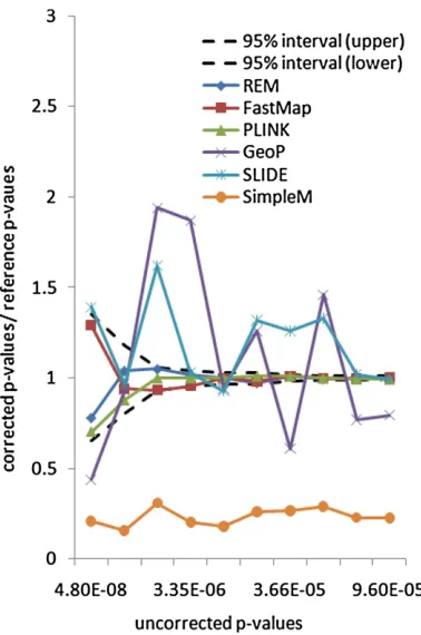
Since this data set only has a very small number of SNPs, the exact methods FastMap and REM can bothfinish within a few hours for 1 million permutations. To evaluate the accuracy of the selected methods, we use the same ratio measurement as in the inbred mouse data set. Figure 4 shows the ratios between the 10 corrected P-values and the referenceP-values (calculated by 100 million permuta-tions) for the selected methods. The uncorrectedP-values of the gene expression traits range from 4.8 ·1028to 9.6 · 1025. After correction, theP-values range from 0.000016 to 0.046. As expected, the corrected P-values of the exact methods all fall into the confidence region. Both GeoP and SLIDE provide overall unbiased permutation P-value
esti-mates. This is because the underlying correlation structure assumption of these approximation methods is appropriate in this yeast data set, as illustrated inFile S1, Figure S1.
Human rare variants
Individual rare variants provide little power for association studies because of their low minor allele frequencies. A commonly used approach is to collapse nearby rare variants and use these collapsed rare variants for association studies (Li and Leal 2008). In this study, we generated a data set of collapsed rare variants on the basis of genotype data from 65 HapMap Yoruba in Ibadan (YRI) samples (Frazer et al.
2007). Specifically, the genotype data of .2 million SNPs were downloaded from the HapMap Web site. Wefirst chose the markers with minor allele frequency,0.05, and no miss-ing values, and then collapsed them within a movmiss-ing window of 50 kb that shifts 10 kb each time. The final data set includes 143,000 collapsed SNPs. We downloaded expression data of these 65 samples (measured by RNA-seq) from the Pritchard laboratory’s Web site (http://eqtl.uchicago.edu/) (Pickrellet al.2010).
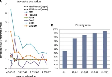
Figure 5A shows the ratios between the correctedP -val-ues and the referenceP-values for the selected methods. The uncorrected P-values of the gene expression traits range from 4.9 · 10210 to 7.1 · 1027. After correction, the P -values range from 8·1026to 0.046. The correctedP-values of the exact methods still fall into the confidence region. For the approximation methods, SLIDE and SimpleM are con-servative for small P-values but become more accurate for
Table 1 Runtime of REM, FastMap, and PLINK on the entire inbred mouse hypothalamus eQTL data
No. resamplings REM (Pt= 0.01) REM (Pt= 0.05) REM (Pt= 1) FastMap PLINK
1,000 2.3 min 4.6 min 13 min 1.2 hr 21 days
10,000 0.3 hr 0.7 hr 2 hr 10 hr 211 days
100,000 2.8 hr 6.7 hr 0.9 day 4 days 5.8 yr
1 million 1.2 days 2.8 days 8.6 days 40 days 58 yr
The data set contains 150,000 SNPs and 3600 gene expression traits over 32 strains. The runtimes.10 days are estimated from smaller-scale experiments.
larger ones. GeoP estimates are overall unbiased but with largefluctuations.
Figure 5B shows the percentage of the SNPs that are pruned by REM under different significance levels. Note that, at significance level 0.01, .95% SNPs are pruned, and only ,5% SNPs need to be examined for their tests values. Compared to FastMap, REM speeds up the process by 20–30 times.
Applying REM to a large sample study through meta-analysis
The computational efficiency of REM comes from the indexing structure. For each entry in the index structure, REM performs a single computation to calculate a bound of the test statistics of all SNPs in this entry. If the number of samples is large, the number of entries in the indexing structure will also be large. This may impair the computa-tional efficiency of the algorithm. This problem may be alleviated by meta-analysis (Munafo and Flint 2004). In contrast to direct analysis of pooled individual-level data, meta-analysis combines the summary statistics from differ-ent studies.
We apply REM to a large sample data set (with 1000 samples) through meta-analysis. The samples are parti-tioned into groups of equal size. For each group, we apply REM to calculate the resampling-based P-values for 1000 simulated phenotypes. For each phenotype, a combined P -value is computed by applying Fisher’s method to the group
P-values (Fisher 1925). The combinedP-values and original
resampling-basedP-values (when using all samples) are al-most perfectly correlated. Specifically, the correlations are 0.99, 0.98, and 0.96 when we partition the samples into 2, 5, and 10 groups, respectively. Therefore, for large sample studies, we can apply REM to groups and combine the P -values by using meta-analysis. The combined P-values are robust estimations of the original resampling-based P -val-ues. More detailed discussion on applying REM to a large sample study through meta-analysis can be found inFile S1.
Discussion
The resampling-based test is widely used to address the multiple-testing correction problem in genetic association studies. Its main disadvantage is the intensive computa-tional burden. In eQTL studies, the computacomputa-tional problem becomes more severe since one needs to correct theP-values for tens of thousands of gene expression traits. In this article, we present a rapid and robust algorithm, REM, that dramat-ically speeds up the process of the exact resampling-based test. It builds a two-layer indexing structure that groups SNPs by their genotypes. By estimating the upper bound of the test statistics for all SNPs within one group, REM prunes away most of the SNPs. Moreover, since usually we are interested only in the expression traits whose corrected
P-values are less than a certain significance level, REM can
further improve the computational efficiency byfiltering out the insignificant expression traits in early stages. Most im-portantly, REM guarantees that we find the exact resam-pling-based P-values even if it performs the actual tests on only a small number of SNPs. REM can be applied to a wide range of resampling procedures. It provides theflexibility to the user to determine the appropriate resampling strategy for the data set under consideration. We use three eQTL data sets to evaluate the performances of several selected algorithms and demonstrate that REM produces accurate estimates of resampling-basedP-values with much less com-putational cost than other alternatives.
We have shown that the performances of approximation methods vary for different data sets with no method being consistently superior to other methods. The approximation methods achieve higher accuracy on the yeast data set than the other two data sets since the correlation structure in the yeast data set matches the assumptions of the approxima-tion methods. However, in inbred mice and human rare variants data sets, nearby markers do not have higher correlations and the heat maps do not show clear banding correlation structure among SNPs (File S1, Figure S1). Therefore, the correlation assumption of the approximation methods is not valid, which leads to their poor performance. Association studies of the low-frequency/rare variants have recently attracted much research attention (Bodmer and Bonilla 2008; Manolio et al. 2009). With the advance of sequencing techniques, we expect in the near future that rare variants will be used in most association studies. Multiple-testing correction for rare variants association is of great research
interest. Since a single rare variant has little power to detect an association signal, a common approach is to collapse the rare variants at a locus so that 1/0 indicates the presence/ absence of any rare variant (Li and Leal 2008; Morris and Zegginic 2010). The collapsed rare variants often do not have strong correlations among nearby loci, which violates the assumption underlying most approximation methods for permutation P-value estimation. To the best of our knowl-edge, this article is the first effort to address the multiple-testing correction problems of rare variant association and our REM algorithm provides an accurate and computation-ally efficient solution for this problem.
There is room to improve the REM algorithm. In this article, we have focused on the cases where genotype data are binary. The general principle used in REM can also be applied to the situation where one marker may have three possible genotypes, which is among our future research directions.
In summary, the REM algorithm provides an efficient solution to calculate the exact resampling-basedP-values for a variety of statistical tests in eQTL studies. It has been demonstrated to be much faster than recently developed methods. The software is implemented in C++ and is pub-licly available athttp://csbio.unc.edu/eQTL. The algorithm can be easily parallelized, for example, by parallelizing the computation for each gene expression trait.
Acknowledgments
This work was partially supported by Environmental Pro-tection Agency grant RD-83382501; National Science Foun-dation awards IIS0448392 and IIS0812464; and National Institutes of Health awards U01CA105417, U01CA134240, and MH090338.
Literature Cited
Barrett, J., B. Fry, J. Maller, and M. Daly, 2005 Haploview: anal-ysis and visualization of LD and haplotype maps. Bioinformatics 21(2): 263–265.
Benjamini, Y., and Y. Hochberg, 1995 Controlling the false dis-covery rate: a practical and powerful approach to multiple test-ing. J. R. Stat. Soc. B 57(1): 289–300.
Bochner, B. R., 2003 New technologies to assess genotype–phenotype relationships. Nat. Rev. Genet. 4: 309–314.
Bodmer, W., and C. Bonilla, 2008 Common and rare variants in multifactorial susceptibility to common diseases. Nat. Genet. 40 (6): 695–701.
Boyd, S., and L. Vandenberghe, 2004 Convex Optimization. Cam-bridge University Press, CamCam-bridge, UK/London/New York. Breitling, R., Y. Li, B. M. Tesson, J. Fu, C. Wuet al., 2008 Genetical
genomics: spotlight on QTL hotspots. PLoS Genet. 4(10): e1000232. Brem, R. B., and L. Kruglyak, 2005 The landscape of genetic com-plexity across 5,700 gene expression traits in yeast. Proc. Natl. Acad. Sci. USA 102(5): 1572–1577.
Brem, R. B., J. D. Storey, J. Whittle, and L. Kruglyak, 2005 Genetic interactions between polymorphisms that affect gene expression in yeast. Nature 436(7051): 701–703.
Browning, B. L., 2008 PRESTO: rapid calculation of order statistic distributions and multiple-testing adjusted P-values via permu-tation for one and two-stage genetic association studies. BMC Bioinformatics 9: 309.
Cheverud, J. M., 2001 A simple correction for multiple compar-isons in interval mapping genome scans. Heredity 87: 52–58. Churchill, G., and R. W. Doerge, 2008 Naive application of
permu-tation testing leads to inflated type I error rates. Genetics 178: 609– 610.
Churchill, G. A., and R. W. Doerge, 1994 Empirical threshold values for quantitative trait mapping. Genetics 138: 963–971. Conneely, K., and M. Boehnke, 2007 So many correlated tests, so
little time! Rapid adjustment of P values for multiple correlated tests. Am. J. Hum. Genet. 81(6): 1158–1168.
Fei, Z., Z. Xu, and T. Vision, 2006 Assessing the significance of quantitative trait loci in replicable mapping populations. Genet-ics 174: 1063–1068.
Fisher, R., 1925 Statistical Methods for Research Worker. Oliver & Boyd, Edinburgh.
Frazer, K., D. Ballinger, D. Cox, D. Hinds, L. Stuveet al., 2007 A second generation human haplotype map of over 3.1 million SNPs. Nature 449(7164): 851–861.
Gao, X., J. Starmer, and E. Martin, 2008 A multiple testing cor-rection method for genetic association studies using correlated single nucleotide polymorphisms. Genet. Epidemiol. 32(4): 361–369.
Gatti, D. M., A. A. Shabalin, T.-C. Lam, F. A. Wright, I. Rusynet al., 2009 FastMap: Fast eQTL mapping in homozygous popula-tions. Bioinformatics 25(4): 482–489.
Good, P., 2005 Permutation, Parametric and Bootstrap Tests of Hypotheses. Springer-Verlag, New York.
Han, B., H. Kang, and E. Eskin, 2009 Rapid and accurate multiple testing correction and power estimation for millions of corre-lated markers. PLoS Genet. 5(4): e1000456.
Kendziorski, C., and P. Wang, 2006 A review of statistical meth-ods for expression quantitative trait loci mapping. Mamm. Ge-nome 17(6): 509–517.
Kimmel, G., and R. Shamir, 2006 A fast method for computing high-significance disease association in large population-based studies. Am. J. Hum. Genet. 79(3): 481–492.
Li, B., and S. Leal, 2008 Methods for detecting associations with rare variants for common diseases: application to analysis of sequence data. Am. J. Hum. Genet. 83(3): 311–321.
Li, J., and L. Ji, 2005 Adjusting multiple testing in multilocus analyses using the eigenvalues of a correlation matrix. Heredity 95(3): 221–227.
Lin, D., 2005 An efficient Monte Carlo approach to assessing sta-tistical significance in genomic studies. Bioinformatics 21(6): 781–787.
Manolio, T., F. Collins, N. Cox, D. Goldstein, L. Hindorff et al., 2009 Finding the missing heritability of complex diseases. Nat. Genet. 461(7265): 747–753.
McClurg, P., J. Janes, C. Wu, D. Delano, J. Walker et al., 2007 Genomewide association analysis in diverse inbred mice: power and population structure. Genetics 176: 675–683. Michaelson, J., S. Loguercio, and A. Beyer, 2009 Detection and
interpretation of expression quantitative trait loci (eQTL). Meth-ods 48(3): 265–276.
Morris, A., and E. Zegginic, 2010 An evaluation of statistical ap-proaches to rare variant analysis in genetic association studies. Genet. Epidemiol. 34(2): 188–193.
Moskvina, V., and K. Schmidt, 2008 On multiple-testing correc-tion in genome-wide associacorrec-tion studies. Genet. Epidemiol. 32 (6): 567–573.
Munafo, M., and J. Flint, 2004 Meta-analysis of genetic associa-tion studies. Trends Genet. 20(9): 439–444.
Nettleton, D., and R. W. Doerge, 2000 Accounting for variability in the use of permutation testing to detect quantitative trait loci. Biometrics 56(1): 52–58.
Nyholt, D. R., 2004 A simple correction for multiple testing for single-nucleotide polymorphisms in linkage disequilibrium with each other. Am. J. Hum. Genet. 74(4): 765–769.
Pahl, R., and H. Schafer, 2010 PERMORY: an LD-exploiting per-mutation test algorithm for powerful genome-wide association testing. Bioinformatics 26(17): 2093–2100.
Pe’er, I., R. Yelensky, D. Altshuler, and M. Daly, 2008 Estimation of the multiple testing burden for genomewide association studies of nearly all common variants. Genet. Epidemiol. 32(4): 381– 385.
Pickrell, J., J. Marioni, A. Pai, J. Degner, B. Engelhardt et al., 2010 Understanding mechanisms underlying human gene ex-pression variation with RNA sequencing. Nature 464(7289): 768–772.
Purcell, S., B. Neale, K. Todd-Brown, L. Thomas, M. Ferreiraet al., 2007 PLINK: a tool set for whole-genome association and pop-ulation-based linkage analyses. Am. J. Hum. Genet. 81(3): 559– 575.
Roberts, A., L. McMillan, W. Wang, J. Parker, I. Rusyn et al., 2007 Inferring missing genotypes in large SNP panels using fast nearest-neighbor searches over sliding windows. Bioinfor-matics 23(13): i401–i407.
Rockman, M. V., and L. Kruglyak, 2006 Genetics of global gene expression. Nat. Rev. Genet. 7: 862–872.
Salyakina, D., S. R. Seaman, B. L. Browning, F. Dudbridge, and B. Müller-Myhsok, 2005 Evaluation of Nyholt’s procedure for multiple testing correction. Hum. Hered. 60: 19–25.
Seaman, S. R., and B. Müller-Myhsok, 2005 Rapid simulation of P values for product methods and multiple-testing adjustment in association studies. Am. J. Hum. Genet. 76(6): 399–408. Storey, J. D., 2003 The positive false discovery rate: a Bayesian
interpretation and the q-value. Ann. Stat. 31(6): 2013–2035. Sun, W., and F. A. Wright, 2010 A geometric interpretation of the
permutation p-value and its application in eQTL studies. Ann. Appl. Stat. 4(2): 1014–1033.
Westfall, P. H., and S. S. Young, 1993 Resampling-Based Multiple Testing: Examples and Methods for P-Value Adjustment. Wiley, New York.
Zhang, X., F. Pan, and W. Wang, 2009 Efficient algorithms for genome-wide association study. ACM Trans Knowl Discov Data 3(4): 19.
Zhang, X., F. Pan, Y. Xie, F. Zou, and W. Wang, 2010 COE: a gen-eral approach for efficient genome-wide two-locus epistasis test in disease association study. J. Comput. Biol. 17(3): 401–415.
GENETICS
Supporting Information
http://www.genetics.org/content/suppl/2012/01/31/genetics.111.137737.DC1
Rapid and Robust Resampling-Based
Multiple-Testing Correction with Application
in a Genome-Wide Expression Quantitative
Trait Loci Study
Xiang Zhang, Shunping Huang, Wei Sun, and Wei Wang
Assumption of Existing Approximation Methods for Multiple Testing Correction
Figure S1 illustrates the correlation structures of genotype data in yeast segregants (BREMet al.2005) (Figure
S1(a-b)), mouse inbred strains (MCCLURGet al.2007) (Figure S1(c-d)), and rare variants in human population (FRAZER
et al.2007) (Figure S 1(e-f)). More details of these three datasets have been discussed in the Results Section. The
yeast segregants data is a typical genetic dataset from a cross of inbred strains where markers within a chromosome are
highly correlated (Figure S1 (a)) and form an approximate banding structure (Figure S1 (b)). Thus this dataset satisfies
the assumptions needed for the approximation methods. In contrast, we do not observe such correlation structure in
the data of mouse inbred strains and human rare variants. Both mouse inbred strains and human rare variants data are
commonly encountered in genetic studies. The insufficiency of the approximation methods for these datasets motivates
the recent development of theexhaustivemethods that calculate the exact resampling-basedP-values.
(a) (b)
(c) (d)
(e) (f)
Figure S1: Difference between correlation structures in the yeast [(a) and (b)], inbred mouse [(c) and (d)], and human rare variant [(e), (f)] data sets. (a), (c), (e) compare the correlation density for marker pairs within and between chromosomes. (b), (d), and (f) are the heat maps of correlation matrices in chromosome 12 of the three data sets.
Convexity of Commonly Used Statistical Tests
It has been shown that most of the commonly used statistical tests in eQTL studies, such as Pearson’s correlation,
Student’s t-test, analysis of variance (ANOVA F-test), and likelihood ratio test are equivalent for binary genotype data
(GATTIet al.2009). Without loss of generality, we show that the ANOVA F-test is a convex function ofY¯1. Recall
thatY¯1is defined as follows: for SNPXn and a resampled phenotypeYmk,Y¯1 represents the sum of the phenotype
values of the individuals with rarer alleles (i.e., whenXnequals to 1).
The ANOVA F-test partitions the total sum of squares SST into a between-group sum of squares SSB and a
within-group sum of squaresSSW. The F-statistic isF =cSSB/SSW, wherecis a fixed constant for a particular
study. LetSST be the total sum of squares. We have thatF =cSSB/SSW =cSSB/(SST −SSB). For a given
resampled phenotype vectorYk
m, the F-statistic is a monotone function ofSSB. From now on, we will useSSBas our
test statistic. For SNPXnand resampled phenotype vectorYmk,
SSB(Xn, Ymk) =
¯ Y2
0 S0
+ ¯ Y2
1 S1 −
¯ Y2
S ,
whereY¯0andY¯1are the sums of the phenotype values inYmk whenXnequals to 0 and 1, respectively,S0andS1are
the numbers of 0’s and 1’s inXn, respectively,Y¯ is the sum of all phenotype values inYmk, andSis the total number
of individuals. Clearly,Y¯0+ ¯Y1= ¯Y,S0+S1=S, and thus we can rewriteSSBas
SSB(Xn, Ymk) =
( ¯Y −Y¯1)2 S−S1
+ ¯ Y2
1 S1
−Y¯2
S . (1)
Clearly,SSB(Xn, Ymk)is a convex function (more specifically a quadratic function) ofY¯1.
Accuracy Evaluation using Synthetic Phenotypes
To further study the accuracy of the selected methods on the inbred mouse data set, we generate three synthetic
phe-notypes whose values follow standard normal, exponential, and uniform distributions. For each synthetic phenotype,
we use the selected methods to correct theP-values. The uncorrectedP-values ranges from1.2×10−9to5.4×10−7
(normal),5.4×10−12to7.6×10−8(exponential), and2.7×10−11to2.1×10−7(uniform). After correction (by
100M permutations), theP-values range from 0.00039 to 0.052 (normal), 0.00044 to 0.053 (exponential), and 0.00026
to 0.05 (uniform). Then we apply different methods to estimate the correctedP-values.
Figures S2(a), S2(b), and S2(c) show the results when using the permutationP-values as reference. From these
figures, we can observe a similar trend using the three synthetic datasets to that using the real expression traits data. The
approximation methods are anti-conservative. Moreover, they do not provide accurate estimation for the permutation
P-values. Their performances vary for phenotypes with different distributions. GeoP does not work for exponentially
distributed phenotypes (with all correctedP-values being 0), though it performs better than SLIDE and SimpleM on
the other two distributions. This demonstrates that the distribution of the phenotypes plays an important role in the
performances of the approximation methods.
(a) Synthetic normally distributed trait
(b) Synthetic exponentially distributed trait (c) Synthetic uniformly distributed trait
Figure S2: Accuracy evaluation of selected methods on synthetic gene expression traits using inbred mouse data set. (Each line represents the ratio between the correctedP-values and the referenceP-values for a method. The reference
P-values are obtained using 100M permutations. An accurate method should yield a ratio of 1. In this figure, the referenceP-values are estimated by permutation test.)
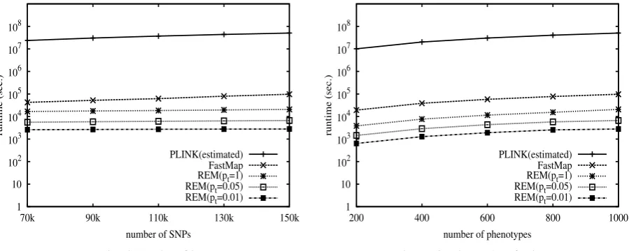
Computational Efficiency Evaluation when Varying the Size of the Data Set
We randomly sample 1K real gene expression traits for the evaluation. Unless otherwise specified, the default
exper-imental setting is as follows: number of SNPs = 150K, number of traits = 1K, and number of resamplings = 100K.
PLINK is not computationally efficient enough for this setting. However, since its runtime is linear to the number of
resamplings, we estimate its runtime for 100K resamplings by first running it with 100 resamplings, and then
multi-plying the runtime by 1000. We examine the runtimes of REM for three different thresholds of correctedP-values, 1,
0.05, and 0.01. When the threshold is set to be 1, REM will find the correctedP-values for all traits. Otherwise REM
automatically finds the traits whose correctedP-values are less than the threshold. As shown in Figure S3, FastMap
is about two orders of magnitude faster than PLINK. REM further improves the computational efficiency by about
two orders of magnitude. The computational efficiency of REM is dramatically improved when the correctedP-value
threshold decreases, because REM can filter out insignificant traits in a very early stage of the process.
1 10 102 103 104 105 106 107 108
70k 90k 110k 130k 150k
runtime (sec.)
number of SNPs
PLINK(estimated) FastMap REM(pt=1) REM(pt=0.05) REM(pt=0.01)
(a) Varying the number of SNPs
1 10 102 103 104 105 106 107 108
200 400 600 800 1000
runtime (sec.)
number of phenotypes PLINK(estimated)
FastMap REM(pt=1) REM(pt=0.05) REM(pt=0.01)
(b) Varying the number of traits
Figure S 3: Efficiency evaluation of three exact methods, PLINK, FastMap, and REM, when varying the number of SNPs and the number of traits in the mouse data set. The y-axis (runtime) is in logarithmic scale. The runtime of PLINK is estimated based on small scale experiments. See text for more details.
Pseudo Code of the REM Algorithm
Algorithm S1: REM - Rapid and Exact Multiple testing correction by resampling
Input: SNPs{X1, X2,· · ·, XN}, gene expression traits{Y1, Y2,· · ·, YM}, number of resamplesK, and desired resampling-basedP-value thresholdpt.
Output: Significant gene expression traits, i.e., the ones whose resampling-basedP-values are no greater than pt.
index SNPs{X1, X2,· · ·, XN}by the two-layer indexing structure;
1
foreveryYm(1≤m≤M)do
2
scan all SNPs to find maximum statisticTYm;
3
generate resampled phenotype vectors{Ym1, Ym2,· · · , YmK};
4
count= 0;
5
pres(Ym) =countK+1+1;
6
foreveryYmk (1≤k≤K)do
7
foreverye1i(e1iis a first layer entry)do
8
ifub(e1i)>TYmthen
9
foreverye2j(e2jis a second layer entry ofe1i)do
10
ifub(e2j)>TYm then
11
foreveryXnin entrye2jdo
12
ifT(Xn, Ymk)>TYmthen
13
count=count+ 1;
14
pres(Ym) =countK+1+1;
15
goto line 23;
16
end
17
end
18
end
19
end
20
end
21
end
22
ifpres(Ym)> ptthen
23
goto line 2;
24
end
25
end
26
returnYmas significant;
27
end
28
Time Complexity of REM
Supposed that we haveSindividuals,N SNPs,M Phenotypes, andKPermutations/bootstrapps. In Line 1 of
Algo-rithm S1, the overall time complexity for indexing the SNPs isO(N S). In Line 9, the total number of upper bounds
in the first layer we need to check is(S/2)2/2. The complexity of each check isO(1). So the overall time complexity
for searching the first layer isO(KM S2). In Line 11, in the worse case, each first layer entry hasO(S2)second layer
entries. However, the total number of secondary entries cannot be larger than the total number of SNPsN. Thus, the
worst case time complexity for searching the second layer isO(KM N). Moreover, in practice, for a first layer entry,
a second layer indexing is only needed when its number of SNPs is larger than the possible number of second layer
entries. Only a small portion of the first layer entries will actually have the second layer indexing. The overall time
complexity of REM isO(N S+KM S2+KM N).
Note that the complexity analysis only provides an asymptotic description of the worst case performance of the
algorithm. The actual performance of the algorithm heavily depends on the tightness of the upper bound, which has
been demonstrated by extensive experimental evaluation.
Applying REM to Large Sample Study through Meta-Analysis
REM can be effectively applied to large sample study through meta-analysis. In a meta-analysis, the samples are
partitioned into several groups. The resampling-based P-values within each group are calculated using REM. The
P-values are then combined by applying Fisher’s method (FISHER1925).
We simulate data sets of large samples to demonstrate the efficacy of REM. We use SNPs in chromosome 22 of
1000 randomly selected individuals from the genome-wide association study of Schizophrenia (SHIet al.2009). At
each locus, the heterozygous genotype is combined with the homozygous genotype of major allele. There are 6,679
SNPs of MAF no less than 0.05. The phenotypesY are simulated by a linear model:Y =Xb+ϵ, whereX is the
genotype of a SNP,bis the coefficient, andϵis the residual error. In our experiments,bvaries from 0.3 to 0.7, andϵ
follows a standard Gaussian distribution.
The square of Pearson’s correlation, R2, is used as the test statistic. We denote the maximumR2 of the
origi-nal phenotype to ber02. The permutationP-value across the 1000 individuals is calculated as the proportion of the
permutations with maximumR2larger thanr20.
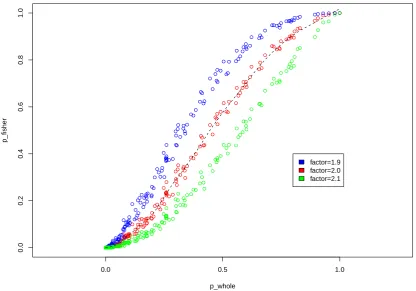
For meta-analysis, we randomly partitioned the data into two groups, each of which has 500 samples. In each
group, we calculated the permutationP-value as the proportion of the permutations whose maximumR2are larger
thanf r2
0, wheref is a constant. We then apply Fisher’s method to combine the permutationP-values of every group
to obtain the meta permutationP-value.
We repeat the above simulation 1000 times and compare the permutationP-values from the whole group (the 1000
individuals) to the meta permutationP-values. Figure S4 depicts that they are highly correlated. Specifically, when
the factorf equals to 2.0 (red points in the figure), the correlation is 0.99.
Meta-analysis using 5 and 10 groups are also performed. The results are similar to that of 2 groups. In particular,
the correlation is 0.98 for 5 groups, and 0.96 for 10 groups.
The nearly perfect correlation between the permutation P-value (of the whole group) and the meta permutation
P-value enables us to apply REM to studies with large samples effectively. Specifically, we first partition the samples
into smaller groups and apply REM to get the permutationP-values for each group. We then combine theseP-values
by the Fisher’s method to get a meta permutationP-value. Finally, we map the meta permutation P-value to the
original permutationP-value following the estimated relationship (e.g., the line corresponding to factor 2 in Figure
S4) between these two values. Note that the relationship between the original permutation P-value and the meta
permutationP-value can be estimated by using a small number (e.g., tens) of phenotypes.
The exact value of the factorfis not essential to the success of our method. This is because, for any given factorf,
we can always estimate the relationship between the meta permutationP-value and the original permutationP-value.
For example, the three lines in Figure S4 correspond to three different values off. Any one of them can be used to
map between the twoP-values. In theory, however, it is interesting to investigate whether there exists an optimalf
value that gives the highest correlation between the twoP-values. This is among our future research directions.
0.0 0.5 1.0
0.0
0.2
0.4
0.6
0.8
1.0
p_whole
p_fisher
factor=1.9 factor=2.0 factor=2.1
Figure S4: Relationship between the combinedP-values and the originalP-values
LITERATURE CITED
BREM, R. B., J. D. STOREY, J. WHITTLE, and L. KRUGLYAK, 2005 Genetic interactions between polymorphisms
that affect gene expression in yeast. Nature436(7051):701–703.
FISHER, R., 1925 Statistical Methods for Research Worker. Oliver and Boyd (Edinburg).
FRAZER, K., D. BALLINGER, D. COX, D. HINDS, L. STUVE, R. GIBBS, J. BELMONT, A. BOUDREAU, P.
HARD-ENBOL, S. LEAL, and OTHERS, 2007 A second generation human haplotype map of over 3.1 million SNPs.
Nature449(7164):851–861.
GATTI, D. M., A. A. SHABALIN, T.-C. LAM, F. A. WRIGHT, I. RUSYN, and A. B. NOBEL, 2009 FastMap: Fast
eQTL mapping in homozygous populations. Bioinformatics25(4):482–489.
MCCLURG, P., J. JANES, C. WU, D. DELANO, J. WALKER, S. BATALOV, J. TAKAHASHI, K. SHIMOMURA,
A. KOHSAKA, J. BASS, T. WILTSHIRE, and A. SU, 2007 Genomewide Association Analysis in Diverse Inbred
Mice: Power and Population Structure. Genetics176(1):675–683.
SHI, J., D. LEVINSON, J. DUAN, A. SANDERS, Y. ZHENG, I. PE’ER, F. DUDBRIDGE, P. HOLMANS, A.
WHIT-TEMORE, B. MOWRY, A. OLINCY, F. AMIN, C. CLONINGER, J. SILVERMAN, N. BUCCOLA, W. BYERLEY,
D. BLACK, R. CROWE, J. OKSENBERG, D. MIREL, K. KENDLER, R. FREEDMAN, and P. GEJMAN, 2009
Com-mon variants on chromosome 6p22.1 are associated with schizophrenia. Nature460(7256):753–757.
![Figure S1: Difference between correlation structures in the yeast [(a) and (b)], inbred mouse [(c) and (d)], and humanrare variant [(e), (f)] data sets](https://thumb-us.123doks.com/thumbv2/123dok_us/1563716.1192175/13.595.124.484.94.635/figure-difference-correlation-structures-inbred-mouse-humanrare-variant.webp)