Distributed Formation Control for Ground Vehicles with Visual Sensing Constraint

(1)

University of Windsor University of Windsor

Scholarship at UWindsor

Electronic Theses and Dissertations Theses, Dissertations, and Major Papers

1-1-2019

Distributed Formation Control for Ground Vehicles with Visual

Sensing Constraint

Jie Tang

University of Windsor

Follow this and additional works at: https://scholar.uwindsor.ca/etd

Recommended Citation Recommended Citation

Tang, Jie, "Distributed Formation Control for Ground Vehicles with Visual Sensing Constraint" (2019). Electronic Theses and Dissertations. 8181.

https://scholar.uwindsor.ca/etd/8181

This online database contains the full-text of PhD dissertations and Masters’ theses of University of Windsor students from 1954 forward. These documents are made available for personal study and research purposes only, in accordance with the Canadian Copyright Act and the Creative Commons license—CC BY-NC-ND (Attribution, Non-Commercial, No Derivative Works). Under this license, works must always be attributed to the copyright holder (original author), cannot be used for any commercial purposes, and may not be altered. Any other use would require the permission of the copyright holder. Students may inquire about withdrawing their dissertation and/or thesis from this database. For additional inquiries, please contact the repository administrator via email

(2)

Distributed Formation Control for

Ground Vehicles with Visual

Sensing Constraint

by

Jie Tang

A Thesis

Submitted to the Faculty of Graduate Studies

through the Department of Electrical and Computer Engineering in Partial

Fulfillment of the Requirements for

the Degree of Master of Applied Science

at the University of Windsor

Windsor, Ontario, Canada

2019

c

(3)

Distributed Formation for Ground Vehicles with Visual Sensing Constraint

by

Jie Tang

APPROVED BY:

M.J.Ahamed

Department of Mechanical, Automotive and Materials Engineering

B.Balasingam

Department of Electrical and Computer Engineering

X.Chen, Advisor

Department of Electrical and Computer Engineering

(4)

Author’s Declaration of Originality

I hereby certify that I am the sole author of this major paper and that no part of this

major paper has been published or submitted for publication.

I certify that, to the best of my knowledge, my major paper does not infringe upon

anyone’s copyright nor violate any proprietary rights and that any ideas, techniques,

quotations, or any other material from the work of other people included in my major

paper, published or otherwise, are fully acknowledged in accordance with the standard

referencing practices. Furthermore, to the extent that I have included copyrighted

material that surpasses the bounds of fair dealing within the meaning of the Canada

Copyright Act, I certify that I have obtained a written permission from the copyright

owner(s) to include such material(s)in my major paper and have included copies of

such copyright clearances to my appendix.

I declare that this is a true copy of my major paper, including any final revisions, as

approved by my major paper committee and the Graduate Studies office, and that

this major paper has not been submitted for a higher degree to any other University

(5)

Abstract

Formation control combined with different tasks enables a group of robots to reach

a geographical location, avoid a collision, and simultaneously maintain the designed

formation pattern. The connection and perception are critical for a multi-agent

for-mation system, mainly when the robots only use vision as a communication method.

However, most visual sensors have limited Field-of-view (FOV), which leaves some

blind zones. In this case, a gradient-based distributed control law can be designed

to keep every robot in the visible zones of other robots during the formation. This

control strategy is designed to be processed independently on each vehicle with no

network connection. This thesis assesses the feasibility of applying the gradient

de-scent method to the problem of visual constraint vehicle formation.

(6)

Dedication

(7)

Acknowledgments

I would like to take this opportunity to thank my supervisor, Dr. Xiang Chen, for

his elaborate guidance through every stage of this research paper. His support and

feedback helped in transforming this paper into a more meaningful one. His immense

passion for teaching and research have further inspired me to pursue this path in the

future.

I would also like to thank my committee members, Dr. Balakumar Balasingam and Dr.

Jalal Ahamed, for their constructive comments, valuable feedback, positive criticism

and their time in reviewing my work.

I would like extend my gratitude to my lab colleagues, Tong Zhang and Youying Hua,

in the Graduate Control and Robotics Lab, for their friendship, support, their constant

involvement, and their valuable feedback.

Finally, I would like to thank my family and friends who continuously aid me in my

research. My parents, Jun Tang and Wenhui Zhang, support me both mentally and

financially, and my friend Zichun Zhao helped me do the experiments on weekends

(8)

List of Tables

5.1 Parameters Used in the Experiment . . . 38

5.2 Parameters Used in the Experiment . . . 40

5.3 MAE of relative positions before turning. . . 45

5.4 MAE of orientations before turning . . . 45

5.5 MAE of relative positions after turning. . . 45

(12)

List of Figures

1.1 A Leader-follower Control Strategy[1] . . . 4

1.2 The Virtual Structure Control Strategy[2] . . . 5

2.1 Fixed Point Rotation Convention . . . 10

2.2 Non-holonomic vehicle model . . . 11

2.3 Camera model transform point from 3D to 2D . . . 14

2.4 The transformation from world frame to camera coordinate . . . 15

3.1 Relative angle between vehicle i and vehicle j . . . 17

3.2 Transition zone used in Jv(s) . . . 20

3.3 Multi-vehicle Formation System with Visual Constraint . . . 22

3.4 The control structure for each vehicle . . . 22

4.1 Project Architecture . . . 25

4.2 The Sketch of Omnidirection Wheel Vehicle . . . 26

4.3 PID Control of Vehicle Base Chassis . . . 27

4.4 The Hardware Structure of Vehicle . . . 28

4.5 The photo of vehicle . . . 29

4.6 The Marker Box Illustration . . . 30

4.7 The Mount of Cameras . . . 31

4.8 The Photos Captured from Two Cameras . . . 31

(13)

LIST OF FIGURES

4.10 Checkerboard Borad for Calibration . . . 34

5.1 The indoor environment with 4 vehicles . . . 36

5.2 A General Setup of the Formation System . . . 36

5.3 A Predefined Formation Pattern Target . . . 37

5.4 Experiment of Different Initial Poses . . . 38

5.5 Path of the Experiment in Fig5.4.(c) . . . 39

5.6 Experiment of formation turning test . . . 40

5.7 Trajectories of all the Vehicles . . . 41

5.8 Orientation of vehicles during the experiment . . . 42

5.9 Velocity of vehicles during the experiment . . . 42

5.10 (a)(b) Formation Error of X and Y Directions before Turning, (c)(d) Formation Error of X and Y Directions after Turning . . . 44

5.11 Relative angle between different vehicles (a) vehicle1&2 (b) vehicle1&3 (c) vehicle1&4 (d)vehicle3&1 (e)vehicle3&2 (f) vehicle3&4 . . . 46

5.12 Final Formation Pattern . . . 47

A.1 The Nvidia TX2 . . . 52

A.2 The Micro-controller . . . 53

A.3 The Camera Module . . . 53

A.4 The Inertia Measurement Unit . . . 54

(14)

List of Abbreviations

FOV Field of View

HD High Definition

IMU Inertial Measurement Unit

MAE Mean Absolute Error

MATLAB Matrix Laboratory

MCU Micro Controller Unit

NVIDIA NVIDIA Corporation

PID Proportional, Integral, and Derivative

PnP Perspective-n-Point

ROS Robot Operation System

UAV Unmanned Aerial Vehicle

(15)

Chapter 1 Introduction

A group of robots needs cooperation when fulfilling a certain task. It has

numer-ous reasons to let robots work cooperatively. Not only efficiency, redundancy, and

flexibility can be improved dramatically, but also, some tasks single robot impossibly

performed are feasible with multi-robots. Although the prospect is attractive, there

are still some scientific and technological challenges. One can imagine the control of a

group of robots, the method of communications among multi-robots, dealing with

un-stable and constraint communicating, etc. These kinds of challenges will be discussed

in following sections, section.1.1 and section.1.2. Also, some popular control

strate-gies of multi-robots cooperation, particularly formation control, will be introduced in

section.1.3.

1.1 Vision-based Formation of Ground Vehicles

Formation control generally refers to the control approach to accomplish a specific

pattern with a group of robots. It is the foundation of autonomous cooperative control

with multi-robots, which can be widely used in surveillance, distributed manipulation,

mapping of unknown environments, and transportation of large objects[3]_{. Formation}

(16)

CHAPTER 1. INTRODUCTION

fusion, embedded systems, and distributed systems.

Meanwhile, depending on whether there is any central controller doing motion

plan-ning and making decisions for all the vehicles, a formation control can be classified

to the central or distributed controller. Distributed control strategy means that the

robots give a response mainly relay on the local information and decisions. The

central operator may exist but only fulfill the supervisory control. Excepting with

the feature of full autonomy, the distributed system also has the following benefits:

(1)The computing can be done parallel. (2)The system will be more robust without

the central controller. (3)The increase of total agent numbers will not dramatically

rise the computing power.

One of the critical aspects of a robotic system is perception. It determines how robots

senses the environment and extract useful information, which usually means the

es-timation of robots’ pose for the formation problem. Vision has long been considered

as one of the most intuitional and powerful means of perception. Visual sensing can

provide sufficient information to perform control tasks. However, the challenge will

come with the fact that real-time control will require a lot of computing power,

espe-cially with distributed onboard computation. Also, the limitation of field of view is

another challenge, which will be discussed later in the next section.

In the 2D case, the ground vehicles can be chosen as an appropriate research

ob-ject. Most of the ground vehicles have nonholonomic kinematics, which constrains

the movement along the side direction. The nonholonomic constraints should also be

(17)

1.2 Field of View Constraint

It is well-known that every sensor has a limitation with the working range and field.

As for vision sensors, the field-of-view (FOV) defines the area of inspection captured

by the camera. It restricts the horizontal and vertical angle as a boundary for

vi-sual sensors. Under the condition of limited FOV constraint, the vivi-sual connection

between every two robots may be unstable during the formation. In some sensing

and communication constraint cases, one of the tasks could be maintaining visibility

among all the vehicles.

In some particular scenarios, the robots need to see all each other simultaneously.

For example, a group of UAVs or robots with bidirectional full vision connections can

prepare defense when any vehicle in formation is getting attacked by the enemy or

invader. Keeping visibility is meaningful for defense-purposed surveillance.

1.3 Literature Review

In recent years, our society has developed an ever-growing interest in autonomous

cooperative agents. Specifically, formation problem has been attracting the most

attention in the multi-agent research field. Based on various criteria, some control

architectures have been constructed in the past few years, such as leader-follower[1,4,5],

virtual structure[2,6,7], behavioural-based[8] etc.

In the leader-follower approach[1]_{, the leader and follower relationships between two}

vehicles are defined. The leaders track the predefined or on-line planned trajectories,

and the followers track leaders based on the relative pose of their nearby leaders.

(18)

com-CHAPTER 1. INTRODUCTION

pared with the followers. Concurrently, the first follower will attempt to maintain

the distance and the orientation with the leaders. Meanwhile, the second follower

will try to track the first follower in the front . The leader-follower approach is easy

to implement and understand. Besides, when leaders are disturbed by external

en-vironments, the formation can still maintain the objective pattern. However, in the

leader-follower approach, the leader vehicles do not have the feedback information

from follower vehicles. A general illustration of the leader-follower approach is shown

in Fig.1.1.

Figure 1.1: A Leader-follower Control Strategy[1]

In[2] a concept of virtual structure is introduced. The author uses virtual structure

to force an ensemble of robots to behave as if they form a rigid body. The control

strategy for virtual structure can be illustrated as a bi-direction control. The

mo-bile robots can be controlled by applying a virtual force field to the whole structure;

also the position and shape of the virtual structure is determined by the action of

each mobile robots. Many considerable works based on virtual structure have been

done in the past few years. In[6]_{, Norman and Hugh decrease the formation error by}

using motion synchronization to modify the trajectory. In[7], formation feedback is

used to improve the robustness of virtual structure formation. The advantage of this

approach is that it is easy to maneuver robots with group behaviour. However, it is

challenging to do extra applications when the formation needs to maintain the virtual

(19)

keep precise formation patterns. A brief illustration of the virtual structure method

is shown in Fig.1.2

Figure 1.2: The Virtual Structure Control Strategy[2]

A behavior-based approach is introduced by considering of doing various tasks, such

as avoiding an obstacle, tracking neighbor vehicles, and formation keeping,

simulta-neously during the formation. Tucker, and Ronald[8] _{used the gain factors to balance}

the importance of different objectives. The combined behavior was generated by

multiplying the outputs of each fundamental objective by its weighting gain, then

summing and normalizing the results. In[9]_{, the initial formation problem combined}

with the navigation task was solved by extending the behavior-based approach with

a navigating algorithm. It is natural to use a behavior-based approach to describe

a formation problem with multiple objectives; however, this approach has

disadvan-tage because the behavior-based approach makes it difficult to analyze the inherent

mathematical properties and prove the stability and convergence.

One of the main challenges for real-time visual-based formation control is the

local-ization of other vehicles. . Locating robots has been an active research topic in recent

years[10] [11] [12]. There are currently two ways for 6D vision-based pose estimations.

The first is solving PnP (Perspective-n-Point) problems[13], which is a traditional way

for visual . The second is deep learning methods[14] _{also become popular in recent}

(20)

for localization.

1.4 Research Objective

The main goal of this thesis is to design a distributed formation system that can

be work with visual constraints. The overall design primarily consists of the vision

localization and distributed local controller.

Three performances will be used as the primary evaluation criteria that will be tested

in the thesis:

1. objective velocity and handing orientation synchronizing,

2. formation pattern convergence and maintenance, and

3. avoidance of blind zones.

1.5 Thesis Outline

This thesis begins with an introduction to the visual-based formation tasks and field

of view (FOV) constraints in chapter 1. Section 1.3 gives some popular formation

control strategies.

Chapter 2. talks about the theoretical foundations used in this thesis. Section 2.1

introduces some basic geometry knowledge that will help to characterize the

forma-tion problem. Secforma-tion 2.2 gives two widely used vehicle dynamic models. Secforma-tion 2.3

presents a brief introduction of graph theory, which is used to describe multi-agent

(21)

will be used to solve the related formation problem in this thesis. Section 2.5 shows

the camera model and visual-based pose estimation method that facilitate

localiza-tion between vehicles.

Chapter 3 introduces the design of distributed formation control system. Section

3.1 outlines the problem formulation of visual constraint formation task . Potential

function design, including visual constraint Cij and formation pattern Vij, and local

controller design are the main components of section 3.2. Section 3.3 presents a

con-trol structure of each vehicle.

Chapter 4 focuses on the details of implementing a formation control system. Section

4.1 presents the general structure of a distributed formation system , and section 4.2

shows the configuration of the vehicles used in the experiment, including the

kinemat-ics, physical performance, and localization method. Software and the library package

used in the project are shown in section 4.3.

Chapter 5 shows the experiment setups and analysis of the results. Introductions

of the experimental environments are given in section 5.1, while random initial pose

conditions are used in section 5.2 to test the convergence ability for different initial

states of the system. In section 5.3, the detailed analysis of experiments is illustrated,

which includes the trajectory, speed, orientation, and relative angles.

(22)

Chapter 2 Theoretical Foundations

To support the some of the mathematical definitions and technical concepts this

thesis utilizes, this chapter will give a brief review of geometry definitions, dynamic

models of vehicle, graph theories, and gradient control. The chapter also introduces

the camera model and pose estimation method.

2.1 Geometry

2.1.1 Euclidean Distance

The Euclidean distance is the most obvious way of representing the distance between

two points in a metric space. The distance between two points X = (x1, x2, ..., xn)

and Y = (y1, y2, ..., yn) in n-dimensional Euclidean space is defined as:

kX−Yk=

v u u t

n X

i=1

(xi−yi) 2

(2.1)

2.1.2 Inner Product

On <2_{, a Euclidean vector is a geometric object that possesses both a magnitude and}

(23)

CHAPTER 2. THEORETICAL FOUNDATIONS

arrow points to. The magnitude of a vector ais denoted by kak. The inner product

of two Euclidean vectors a and b is defined by

a·b =kakkbkcosθ (2.2)

Where θ is the angle betweena and b. It also can be calculated by

θ= arccos a·b

kakkbk (2.3)

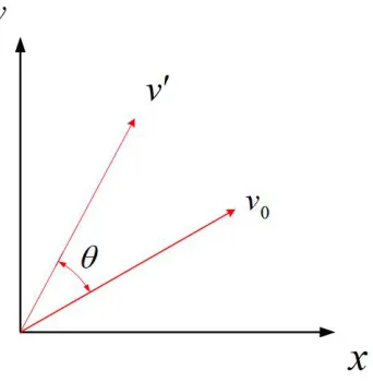
2.1.3 Rotation Matrix

A rotation matrix R in Euclidean n-space is a n×n real orthogonal matrix, whose transpose is its inverse,i.e. RT = R−1,and it determinant det(R) = 1. The product of two rotation matrices is still a rotation matrices. On <2_{, the standard rotation}

matrix has the following form:

R(θ) =



 

cosθ −sinθ

sinθ cosθ





 (2.4)

whereθmeans that a vector has a counterclockwise rotation through angleθ. A given vector v0 = [x, y] rotated by a counterclockwise angleθ in a fixed coordinate system

can be represented by:

v0 =R(θ)v0 (2.5)

Which is also shown in the Fig.2.1.

(24)

Figure 2.1: Fixed Point Rotation Convention

2.2 Dynamic Model of Vehicles

The dynamical model of vehicles plays a crucial role in the formation control

prob-lem. In real world vehicle systems, there are different types of vehicle models, like

holonomic model, nonholonomic vehicle model, Euler-Lagrange vehicle model, and

high-order dynamic model[15]_.

In holonomic vehicle systems, the motion of a vehicle in every axis is independent with

each other. Thus, the vehicles can directly go to any position without constraints.

The general expression of a holonomic vehicle is

˙

pi =vi, v˙i =ui, i∈ {1, . . . , N} (2.6)

Where pi, vi ∈ <n ,n ∈ {2,3}, are the position and the velocity vectors of vehicles. ui

(25)

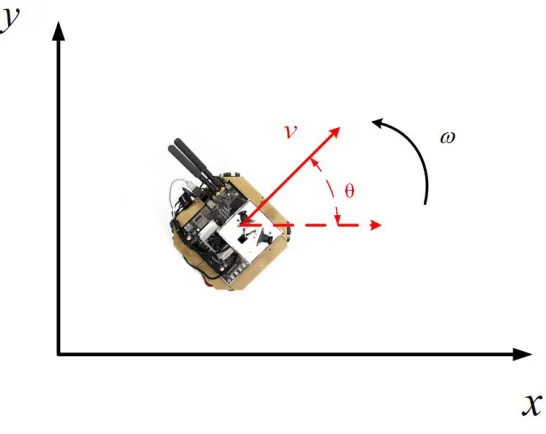
For nonholonomic models, the model on<2 _{is generally given by}

     

    

˙

xi =vicosθi

˙

yi =visinθi

˙

θi =ωi, i= 1, . . . , N

(2.7)

Where the vi, θi and ωi are linear velocity, handing direction and angular velocity

respectively. The vehicle position in world frame is presented by pi =|xi, yi| >

∈ <2_.

A general illustration of nonholonomic vehicle model is shown in Fig.2.2

Figure 2.2: Non-holonomic vehicle model

2.3 Graph Theory and Terminology

Basic concepts of graph theory can be found in any graph theory books[16] [17]. In this

section, it will introduce the modeling of multi-vehicle systems by using graph theory.

(26)

1,2...N. Where theV ={1,· · · , N}andE ={(i, j)|j ∈Ni, i, j ∈V, i6=j}represent

the vertex and edge sets of graph G separately. Each vehicle is an element included

in the vertex set V. Also, the edge set represent connections among the vehicles.

The connections can be direction or undirected connection. For example, if the

connections between two vehicles 1 and 2 is undirected, it means both the vehicle

1 and 2 can receive the information from each other. A neighbor set Ni is used to

characterizing the connection with vehicle i. The graph set,Gf _{= (}_V_,_Ef_{), is used to}

represent desired formation patterns and relation shapes.

2.4 Gradient Formation Control

Gradient formation controllers are based on the gradient descent optimization

algo-rithm, which can find the minimum of a function by using iteration methods. For

a general formation control case, consider the formation of n vehicles with typical

holonomic dynamic 2.6 and a graph pattern G. Between arbitrary two vehicles has

an edge Eij where a corresponding potential function (cost function)Vij can be

con-structed. When these two vehicles are at the desired relative position, the potential

function Vij gets the global minimum value. A typical potential function Vij could

have the following conditions[18] _.

Vij :Rm →R≥0 is continuously differentiable (2.8)

Vij = 0⇐⇒ kpi−pjk=dij (2.9)

∇piVij = 0⇐⇒ kpi−pjk=dij (2.10)

Where the dij is the desired relative position between the vehicle iand vehiclej. ∇x

is defined as∇x ,

h ∂ ∂x1, . . . ,

∂ ∂xm

iT

, in 2D case∇pi = h ∂ ∂xi, ∂ ∂yi iT

(27)

edges inside the graph, the potential function can be defined as :

V = X

(i,j)∈E(t)

Vij (2.11)

Thus, a gradient descent controller for each vehicle can be defined as:

ui =−∇pi X

(i,j)∈E(t)

Vij (2.12)

It has been proved in[19] [20] _{that the formation will finally converge to the desired}

patternGf. If all the conditions (2.8),(2.9),(2.10) are satisfied.

Sometimes developing the potential functions is a kind of art. Different functions are

needed according to various scenarios and tasks.

2.5 Camera Model and Pose Estimation

There are different types of camera models. Take the most common pin-hole cameras

for example. A camera model can be divided into intrinsic and extrinsic parts. The

intrinsic parameters characterize the pin-hole camera model and lens distortion. The

extrinsic matrix includes the translation and rotation of cameras respect to the world

frame[21]_.

The camera model can characterize transformations from a 3D world frame to a 2D

image plane. Here using K to represent the intrinsic matrix[22]_{. Where [}_p

(28)

translation vector which indicates the offset of 2D points in a image plane.

      xpix ypix 1       =K       Xc Yc Zc      

, W hereK=      

fx 0 px

0 fy py

0 0 1

     

| {z }

intrinsic matrix

(2.13)

Where [xpix, ypix]T represents a point in camera image planes (pixel coordinates),

[Xc, Yc, Zc]T represents a point in 3D camera coordinates.

Figure 2.3: Camera model transform point from 3D to 2D

Distortion caused by optical components in the camera is another problem in real

world image systems. The distortion of an image can be characterized by using a

mapping function D, [xdistorted, ydistorted]T =D([xideal, yideal]T) :

xdistorted =xideal(1 +k1?r2+k2?r4+k3?r6)

ydistorted =yideal(1 +k1?r2 +k2?r4+k3?r6)

(2.14)

Where [xdistorted, ydistorted]T represents the point in distorted images, [xideal, yideal]T

means the point in ideal images. rexpresses the distance to the image center,k1, k2, k3

are distortion factors, which respect to different camera and lens.

(29)

is represented by the rotation matrixRand translation vector t. The transformation

from world frames Pw to camera coordinates Pc is shown in(2.15) and Fig.2.4.

Figure 2.4: The transformation from world frame to camera coordinate

Pc= [R|t]Pw (2.15)

Combining the (2.13),(2.14),(2.15), the transformation from world coordinates to

im-age planes can be established in (2.16).

      xpix ypix 1      

=D(K       xc yc zc      

)=D(K[R|t]          Xw Yw Zw 1          ) (2.16)

In (2.16), the intrinsic parameters, D, and K can be identified by doing camera

calibration and the Pw can be known by using prior designed artificial features.

(30)

Chapter 3 Distributed Formation System

Design

This chapter will include the mathematical expression of visual constraint formation

problems, the solution to such a problem, and a control system designed to solve

these problems.

3.1 Problem Statement

The overall objective of this thesis is to create a distributed formation system working

under visual field constraint, with no network information exchange. To express the

visual field constraint, arelative angle γij between the vehicleiand jis introduced

based on (2.3).

cosγij ,f(pi−pj, θj) = 

 

−cosθj

−sinθj    T ·   

xi−xj

yi−yj   

−cosθj

−sinθj

xi−yj

(31)

CHAPTER 3. DISTRIBUTED FORMATION SYSTEM DESIGN

Figure 3.1: Relative angle between vehicle i and vehicle j

Where thepi = [xi, yj]T represents the position of vehicle i in the world coordinate,θj

expresses the heading direction of vehicle j. An illustration of relative angle is shown

in the Fig.3.1. A blind angle α dividing blind zone equally is imported for the sake of simplicity.

It is obvious that when cosγij < cosα, γij > α. It means vehicle i is outside

the blind zone of vehicle j. So the neighbor set of vehicle i is expressed by Ni = {j ∈V|cos (γji)<cos(α),kpj −pik< Rs, j 6=i}. This neighbor set Ni indict the

robot j within the visible zone of robot i.

Thus, two objectives are established, which are keeping the visibility among all

vehi-cles and driving the vehivehi-cles to a desired formation set. The corresponding expressions

are shown:

Objective 1 The restrict {cosγij < cosα,kpj−pik < Rs, j 6= i} holds for all

(32)

camera.

Objective 2The lim

t→∞||(pi−pj)−(hi−hj)|| →0, and θi →θf satisfied fori, j ∈Gf.

Where thehi−hj is the desired relative position in world coordinate for vehicle i and

j.

3.2 General Solution

Based on the section 2.4 and 3.1, one of an appropriate way to solve the

forma-tion control problem is finding a suitable potential funcforma-tion under the given scenario

constraint. In[23]_{, a potential function with visibility constraint has been proposed.}

3.2.1 Potential Function

The potential function were divided into two parts in the paper[23],Vij andCij, which

is shown in (3.2). The Vij focuses on the formation pattern convergence, and the Cij

represents the task of visibility maintenance. kc and kv are two weighting factors to

balance the Cij and Vij

J =

N X

i=1

(kc X

(i,j)∈_E(t)

Cij +kv

X

(i,j)∈_Esub(t)

Vij) (3.2)

Where Esub(t) means a sub edge set, which vehicle i and j inside it is in a visible zone within the distance r . r is a design factor given by Rs−r

(33)

max{||hi−hj||}. The expression of Esub(t) are shown in below.

1.Esub(0) =E(0)∩Ef

2.Esub(t+) =Esub(t−)∪ {(i, j)| kpi(t)−pj(t)k ≤r ,cos (γji(t))<cos(α), i, j ∈V)}

(3.3)

The cost function Vij is presented

Vij =   

 

k(pi−pj)−(hi−hj)k2

kpi−pjk2 ,kpi−pjk ∈(0,khi−hjk] k(pi−pj)−(hi−hj)k2

(Rs−kpi−pjk)2 ,kpi−pjk ∈(khi−hjk, Rs)

(3.4)

It is obvious that the equation(3.4) satisfies the requirements, (2.9), and (2.10). More

over it also has lim

kpi−pjk→0Vij(pi−pj) = +∞and kpi−limpjk→RsVij(pi−pj) = +∞, which

prevent the vehicle i collision with vehicle j or excess visibility distance.

The cost functionCij is represented byCij =ρ(kpi−pjk)Jv(γji), whereρ(kpi−pjk)

is a smooth function to avoid effects ofJv(γji), when a sudden change ofG(t) happen.

Jv(γji) is used to drive vehicles goes out the blind zone(3.5).

Jv(s) =           

0, s > β

Rs β

cosβ−cos(τ)

cos(α)−cos(τ))3dτ, s∈(α, β]

Rs

β ∞, s ∈[0, α]

(3.5)

In the (3.5), a transition zone is defined by usingαandβ. Whenγij is in the transition

(34)

Figure 3.2: Transition zone used inJv(s)

The ρ(kpi−pjk) is given by

ρ(kpi−pjk) =           

1, kpi−pjk ∈[0, r)

1 2

1 + cosπkpi_Rs−pj₋k−_r r, kpi−pjk ∈[r, Rs]

0, kpi−pjk ∈[Rs,∞)

(3.6)

3.2.2 Local Controller

The controller designed by (2.12) can only be directly used in the vehicle having

holonomic kinematic model. Thus, a method convert the gradient to linear and

angular velocity need to be proposed[23].

vi =−sgn

∂J ∂xi

cos (θi) +

∂J ∂yi

sin (θi)

k∇iJk+v0

ωi =

∂J ∂xi

sin

θi+θf

2 − ∂J ∂yi cos

θi+θf

2

v0

−sin

θi−θf

2

(35)

Where ∇iJ = [_∂xi∂J,_∂yi∂J]T. And sgn(s) is a signum function defined as:

sgn(x) :=

          

−1 if x <0

0 if x= 0

1 if x >0

(3.8)

The convergence ability of the proposed local controller in (3.7) is proved in[24] _by

Lyapunov method and a detail derivation is given in the page57 Appendix C. It is

obviously that

∂J ∂xi

= ∂J

∂yi

= 0 → vi =v0 (3.9)

And when _∂xi∂J = _∂yi∂J = 0 & θi =θf the ωi = ˙θi = 0.

3.3 System Design

3.3.1 Distributed Multi-vehicle System

Due to the communication is restricted, and each vehicle is seen as an individual

unit. Thus, a distributed system are constructed to verify the control algorithm. In

a distributed environment each vehicle perceives environments and makes decisions

independently. All the setup related with the experiments are predefined inside in

each vehicle include relative positions, desired velocity, handing, etc.

A general illustration of the multi-vehicles formation system is shown in the 3.3. With

N vehicles included, the system can be established to test the effectiveness of

(36)

Figure 3.3: Multi-vehicle Formation System with Visual Constraint

3.3.2 Embedded System Design

Based on (3.7), a local controller can be designed to maintain the formation pattern

which only relay on the information explored by itself. Thus, we can focus on design

control for each vehicle individually.

Figure 3.4: The control structure for each vehicle

Combining the previous results with a real word sensing environment scenario,

(37)

illustra-CHAPTER 3. DISTRIBUTED FORMATION SYSTEM DESIGN

tion of control structure is shown in Fig3.4 . The whole structure can be divided into

three parts (1) Percetion (2)Planning (3)Control. In the percetion section,the IMUs

are used to get the heading direction of themselves, and cameras are used to resolve

the relative pose between vehicles. In the planning part, based on the pre-processing

information from last step, the _∂xi∂J and the _∂yi∂J are are calculated. In the flow chart

the Cij is given by (3.5)and(3.6), Vij is given by (3.4) respectively. As long as the

robot j is detected by the robot i, we calculate Cij and only when (i, j)∈Esub(t) the

Vij is included in the cost function. The control part is responded for regulation the

(38)

Chapter 4 Implementation Detail

This chapter will introduce the setup of experiment equipment and the development

of software.

4.1 Overview of Vehicle Setup

It is a comprehensive work to design an embedded system including variety of

dif-ferent architecture, such as software and hardware, which need cooperation to get

decent performance. According to needs of visual formation, the primary task of the

project is setting a platform with appropriate hardware and open-source software that

can be used to test formation algorithm in indoor environments. Priority is give to

the object recognition and pose estimation. It is essential to the existing formation

framework in section 3.3 for on-board autonomous control .

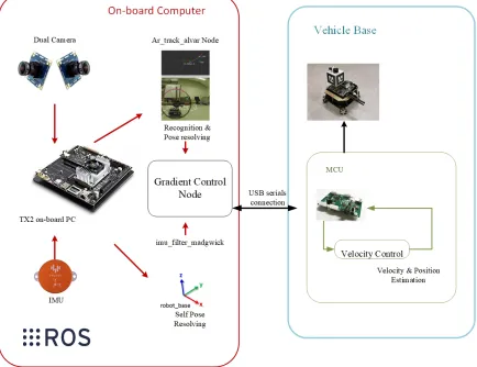
Fig.4.1 is a general architecture that briefly illustrate the main components used in

this project. The main program runs on NVIDIA TX2 with Linux system. Robot

Operation System[25] _{(ROS) are used to fulfill high-level action which finally send the}

(39)

CHAPTER 4. IMPLEMENTATION DETAIL

motors control. The detailed features will be talked in the following sections.

Figure 4.1: Project Architecture

4.2 Configurations of the Vehicle

Each vehicle is seen as one basic unit for the formation system. It is necessary to

consider the kinematics and some on-board sensor performance of the vehicle.

4.2.1 Vehicle Kinematics and Control

Nowadays, there are several of different kinematic models for vehicles, such as,

differ-ential two wheels, omnidirectional, ackerman, mecanum, etc. In this experiment, four

(40)

omnidirectional wheel vehicles is shown in Fig.4.2. With the φ = 45◦ in graph.4.2, the wheels are orthogonal. The forward and inverse kinematic models[26] _{of the}

om-nidirectional vehicles are shown below (4.1),(4.2):

Figure 4.2: The Sketch of Omnidirection Wheel Vehicle

Vr =            vx vy ω            = 1 4      

−√2 −√2 √2 √2

√

2 −√2 −√2 √2 1 L 1 L 1 L 1 L                        v1 v2 v3 v4                  (4.1)

Vw=                  v1 v2 v3 v4                  =         

−√2 2

√ 2 2 L −√2

2

−√2 2 L √

2 2

−√2 2 L √ 2 2 √ 2 2 L                     vx vy ω            (4.2)

WhereVw = [v1 v2 v3 v4]T,v1 v2 v3 v4 are the wheel velocities in the active direction. Vr = [vx vy ω]T,vx and vy are the translational velocities of the robot center, ω is

(41)

this thesis, we only use the vx as linear velocity and ω as angluar velocity to control

the vehicle. There is no vy included in high-level control part.

For the velocity control of chassis, four PID controllers are used to track the desired

linear and angular velocities by controlling four motor drives. An illustration of the

low-level velocity control is shown in 4.3.

Figure 4.3: PID Control of Vehicle Base Chassis

4.2.2 Vehicle Specifications

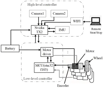
The hardware structure of vehicles are shown in Fig.4.4. The control units of vehicles

are divided to two parts: (a) Master Controller used as a High-level controller (b)

Servo controller used as a low-level controller. The low-level controller is a customized

board based on STM32f103RCT6, which is used to drive the motors according to the

linear and angular velocities sent from high-level controller, meanwhile, resolve the

real-time linear and angular velocity based on encoder data. The NVIDIA TX2

de-veloper board is used as the High-level controller. All computing power consuming

programs are calculated on TX2, like image processing and motion planning.The

NVIDIA TX2 controls the vehicle just by sending linear and angular velocity to the

(42)

including two cameras and IMU. The laptop is used to control all vehicles start/stop

or trigger special event, like changing heading direction.

Figure 4.4: The Hardware Structure of Vehicle

A picture of the omnidirectional vehicles used in this thesis is designed and

con-structed as illustrated in Fig.4.5. Each side of the vehicle is 260mm, the height of the vehicle is 340mm, and the motor drives and controller are placed in the space between the platform and ground. With the selected motor and arrangement mechanism, the

vehicles have maximum linear and angular velocity 1.2 m/s and 5.3 rad/s respectively.

(43)

Figure 4.5: The photo of vehicle

4.2.3 Localization System

Localization system here means both the vision capture method and the features used

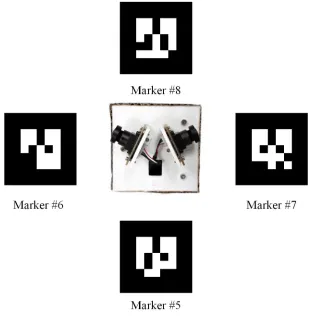
for recognition. This vehicle equipped a marker box with four markers mounted on

the top, which is used as the artificial features to identify different vehicles and do

the localization as shown in Fig.4.5. By using four orthogonal markers, the vehicle

can be detected in any direction An illustration can been found in Fig.4.6.

Each marker forms 90 degree angles with two adjacent markers. Also, the markers on

every surface are unique for the convenience of identification the nubmer and heading

of the vehicles. As shown in Fig4.6, taking vehicle 2 for example, the marker 5 is on

the back of the marker box. When other vehicles get the relative handing of marker

(44)

Figure 4.6: The Marker Box Illustration

To mimic a super wide angle fish-eye camera, two cameras are mounted in opposite

direction with a 170◦ horizontally angle of view and the rotation angle θl =θr = 60◦

which leaves an angle of 70◦ for blind zone as shown in Fig.4.7. In Fig.4.7, the green

areas represent visible zone, the red represent the blind zone. The resolution for each

camera is full HD 1920*1080 and support 30 fps at 1920*1080 mode. A demonstration

of the photo captured by two cameras mounted on the vehicle is shown in Fig.4.8.

The green areas in Fig.4.8 represent the overlap area captured in both two cameras

(45)

Figure 4.7: The Mount of Cameras

(46)

4.3 Software Environments

This section will introduce the software environments and the packages or libraries

used in the thesis will be introduced.

4.3.1 ROS

ROS is the abbreviation of RobotOperatingSystem and ROS is a distributed

frame-work for developing and testing robotics software or algorithms[27]. It provides bunch

of services, including hardware abstraction, low-level device control, implementation

of commonly-used functionality, message-passing between processes, and package

management. ROS has a distributed developing and running structure. By Using

the publish-subscribe mechanism, each node (program or process) can subscribe to

so-called topics and push message to others. ROS also provide the data recording

package named rosbag. By using rosbag, it is easy to record different types message

data for late analyzing like, image and odometer. Hence, the control of autonomous

vehicle is mainly developed and ran on ROS.

4.3.2 Ar_track_alvar

Ar_track_alvar is a package in ROS based on ALVAR library. ALVAR is a

suite of SDKs and products that help researchers and engineers to create augmented

reality applications[28]_{. In} _{Ar_track_alvar}_{, it provides the fast object recognition}

and tracking through fiducials. The fiducials or markers can be also generated with

Ar_track_alvar, which looks like QR-code. The markers with several features help

to be detected, such as clear border and unique pattern. Combined with the prior

knowledge, the size of markers and camera intrinsic matrix, the 2D image plane will

be transformed to 3D world frame. Thus, a 6 DoF pose estimation can be realized in

(47)

Figure 4.9: A Visualization Demo of Ar_track_alvar

Fig.4.9

4.3.3 Camera Calibrator

Camera_calibrator is a camera calibration tool in ROS based on OpenCV camera

calibration library[29]_. _{Camera_calibrator} _{allows easy calibration of monocular or}

stereo cameras using a checkerboard calibration target. A demo of using checkerboard

to calibration is show in Fig.4.10.

4.3.4 MATLAB

Matlab(matrix laboratory) is one of the most widely used numerical computing

envi-ronment. In this thesis, Matlab is used for reading and analyzing the data recorded

(48)

Figure 4.10: Checkerboard Borad for Calibration

4.3.5 Other Libraries and Packages

Some libraries and packages used in the project are briefly introduced in the following.

Gscam[30]based on gstreamer library is used as camera driver in the project. Rosbag[31]

is a set of tools for recording from and playing back to ROS topics. A remote control

node, udp_server, is programmed with universal UPD protocol to receive command

from the laptop. Imu_complementary_filter[32] is imported to fuses angular

ve-locities, accelerations, and (optionally) magnetic readings from a generic IMU device

into a quaternion. Rosserial[33] is a set of library used to communication between

(49)

Chapter 5 Experiments and Result Analysis

In this chapter, the procedure of experiment will be introduced and results will also

be analyzed. In order to test the performance and effectiveness, some different initial

poses, heading directions, and desired velocity conditions are configured during the

experiments. The stability, visual constraint and the synchronization of linear and

angular velocity will be evaluated as the system performance.

5.1 Indoor Environment

All the experiments are finished in the indoor environment with no global localization

information can be used. In Graduate Control and Robotics Lab shown in Fig5.1, it

shows the environment to test the convergence ability and another long range turning

experiment for testing visual constraint using the aisle on the 1st floor in Center for

Engineer Innovation (CEI).

A general setup can be seen in the Fig.5.2. With the number of N vehicles in the

system, each vehicle is set to run independently. By using the UDP protocol, the

laptop computer is only used to send command to start, end the experiment and

(50)

CHAPTER 5. EXPERIMENTS AND RESULT ANALYSIS

Figure 5.1: The indoor environment with 4 vehicles

direction.

To test the system, a set of random initial poses are chosen to only test the

con-vergence and a set of neat initial patterns are chosen to analysis several kinds of

performance. However, the initial pose for G(0) should be connected.

(51)

The desired formation pattern in these two experiments are setting to be a

parallel-ogram shape, which satisfy the visual constraint. A sketch of the desired formation

pattern is shown in the Fig.5.3. The relative position for two experiments in world

frame are set toh1 = [0 0]T, h2 = [0.7 0.4]T,h3 = [1.4 0]T,h4 = [2.1 0.4]T.

Figure 5.3: A Predefined Formation Pattern Target

5.2 Random initial position

In order to test the convergence ability, several sets of initial positions are chosen

which can be seen in Fig.5.4. Some parameter used in the experiments are listed in

the Table5.1. The video containing whole process of three different initial poses is

upload on the following website address.

https://youtu.be/Tp5egQl2Bg0.

In Fig.5.4, it also shows some screen shots in this video with corresponding time.

In Fig.5.4(a), Fig.5.4(b) and Fig.5.4(c), the experiments are using 3 different inital

poses.Form the video and Fig.5.4, it can be notice that, in the most of case, the

formation can converge to the desired pattern within 10 seconds. And a path record

(52)

α

(factor indicate the bland zone)

35

◦

k

_c

(weight factor of

C

_ij

)

0.12 k

v

(weight factor of

V

ij

)

0.2

v

(boundary of transition zone)

0.5 R

s

(maximum visual distance)

5m

r(design factor of range)

3m

θ

_f

(desired heading angle)

90

◦

v

0

(desired velocity)

0 .

2 m/s

Table 5.1: Parameters Used in the Experiment

(53)

Figure 5.5: Path of the Experiment in Fig5.4.(c)

5.3 Long Range Turning Test

In this experiment, the vehicles will change to different heading direction to test the

visual constraint and the influence under disturbance of changing objective target.

Considering the convenience of analysis the performance, a set of straight line initial

position z1 = [0 0 90◦]T,z2 = [0.5 0 90◦]T,z3 = [1 0 90◦]T,z4 = [1.5 0 90◦]T is chosen.

In the experiment, vehicles begin with an objective heading direction θf1 = 90◦ first.

After all robots converged into the desired formation and direction, we change the

objective handing direction to θf2 = 135◦ . All parameters used in the experiment

are listed in the Table.5.2.

The full experiment process can be seen at

https://youtu.be/5x1tOIw7TJc

(54)

α

(factor indicate the bland zone)

35

◦

k

_c

(weight factor of

C

_ij

)

0.08 k

v

(weight factor of

V

ij

)

0.12

v

(boundary of transition zone)

0.5 R

s

(maximum visual distance)

5m

r(design factor of range)

3m

θ

_f₁

(heading before turning)

90

◦

θ

f2

(heading after turning)

135

◦

v

0

(desired velocity)

0 .

2 m/s

Table 5.2: Parameters Used in the Experiment

(55)

5.3.1 Result Analysis

The result are retrieved from the odometer of each vehicle separately. By adding the

initial offset, the trajectories of all the vehicles are collected together in Fig.5.7. And

the orientations and velocities of four vehicles are illustrated in Fig.5.8 and Fig.5.9

separately.

(56)

Figure 5.8: Orientation of vehicles during the experiment

(57)

From the Fig.5.8 and Fig.5.9, it can be noticed that the orientation angles of all

ve-hicles fluctuate around the desired handingθf1 = 90◦ before turning, and around the

θf2 = 135◦ after changing desired heading direction. And the velocity of all vehicles

fluctuate around the desired velocityv0 = 0.2m/sboth before and after changing the

objective handing angle.

The Formation errors corresponding with the desired pattern are shown in the Fig.5.10.

Fig.5.10(a),(b) are the formation errors of X and Y axis with world coordination

(58)

(a) (b)

(c) (d)

Figure 5.10: (a)(b) Formation Error of X and Y Directions before Turning, (c)(d) Formation Error of X and Y Directions after Turning

From table5.3 to 5.6, it collects all the mean absolute errors of relative positions and

orientations in steady states both before and after the turning action.

In Fig.5.11, the relative anglesγij are illustrated in the view of vehicle 1 and 3. All

rel-ative angles are larger than 35◦ during the whole formation procedures which means

(59)

Mean Absolute Error

Position[m]

Vehicle#

1&2

2&3

3&4

X

0.0126

0.0684

0.0077

Y

0.0429

0.0552

0.0530

Table 5.3: MAE of relative positions before turning.

Orientation[

◦

]

Vehicle#

1

2

3

4 Yaw

1.1758

0.7120

1.5396

1.0856

Table 5.4: MAE of orientations before turning

Mean Absolute Error

Position[m]

Vehicle#

1&2

2&3

3&4

X

0.0137

0.0418

0.0456

Y

0.0622

0.0246

0.0863

Table 5.5: MAE of relative positions after turning.

Orientation[

◦

]

Vehicle#

1

2

3

4 Yaw

1.0761

0.7887

0.9335

0.8803

(60)

(a) (b)

(c) (d)

(e) (f)

(61)

A final pattern of the relative position is shown in the Fig5.12, which is coincident

with the objective pattern.

Figure 5.12: Final Formation Pattern

5.4 Conclusion

From these two experiments, it can be seen the formation can converge to and

main-tain a desired pattern with the connected initial graph. In section 5.3 The velocities

and orientation angles of all vehicles can also synchronize to the objective valuev0 and

θf. During this process, the visual constraint also can be satisfied and no collisions

occur among the vehicles. Overall this distributed system can solve the restriction

formation problem.

From the experiment results in graph Fig.5.8 to Fig.5.11, we can notice there are some

(62)

from several places. The fluctuation may from the residual of gradient at the global

minimum of potential function, and insufficient control frequency. The stabilizing

error may mainly from the visual system error, recording error of odometer, and

(63)

Chapter 6 Conclusion

6.1 Overall

A gradient-based control method for formation problem has been developed which

converges well, provides synchronized orientations and velocities, while keeps visual

connections. This provides a base upon which can develop some high-level

applica-tions like surveillance, multi-agent cooperation.

Currently, the algorithm shows that it is feasible for a distributed multi-agent system

to fulfill self-driving formation under visual restriction. Moreover, a part of nature in

this thesis is to give a generalized framework to solve a series of these problems, which

is an optimization task under the special restriction or some certain constraints. A

basic conceptualization will be introduced in the Section6.2.5.

The major implementation drawback is the steady error and fluctuation. Improving

this situation can be a future work on using more powerful hardware and improving

algorithm. Such as a more accuracy camera calibration method can decrease visual

(64)

CHAPTER 6. CONCLUSION

6.2 Future Works

6.2.1 Precise Control Algorithm and Accuracy

Now the distributed control algorithm implemented on each vehicle is absolutely

independent. A synchronized control strategy may be worth to have a try on low

control frequency and computation power limitation situation. The computing can

be still finished on the vehicles individually, meanwhile, some synchronized method

can be added to unify the motion of whole group. The most intuitional way is adding

the synchronized clocks[34]_.

6.2.2 Relaxing the Connection Constraint

Currently, the connection between vehicles is a strong fully connected structure. It is

not necessary to make and maintain the formation with such a strong condition. The

pattern will has more variety if the assumption of fully connection can be relaxed.

Thus, some vehicles can stay in the blind zone of others. Such a relaxation should be

possible to use the existing gradient based controller essentially unmodified, requiring

only some modification on the definition of sub graph Gsub and the graph G which

are used for calculating Cij and Vij .

6.2.3 Non-artificial feature based Localization

It is desirable for the formation system to recognize and localization based on the

nature feature or object rather than the artificial markers. Such an adaption is

feasible with the neural network and deep learning technique[35]_{. It will definitely be}

(65)

6.2.4 Aerospace Vehicle Formation

Aerial vehicles can provide more flexibility for variety of tasks and have the 3D motion

capability. It will be a challenge to develop a neat distributed formation strategy in

3D scenario. Lie group and Lie[36] _{algebra might be a good way to characterize this}

kind of problems.

6.2.5 Basis of Formation Problem

The ultra goal should be developing a framework which allows solving most of the

(66)

Appendix A

Equipment

A.1 on-board computer –Nvidia TX2

The on-board computer is responsible for those computation consuming calculations,

which may include processing sensor information, proposed algorithm calculation and

network connection. Here the Nvidia TX2 are used in the project which is a

power-efficient high performance embedded device with GPU inside.

Figure A.1: The Nvidia TX2

A.2 Low-level Microcontroller

The low-level controller used in the project is a STM32 based customized controller,

(67)

convert chip. The microcontroller board response for resolving the control command

and converting to the speed on each motor,meanwhile, calculate the real velocity

based on the encoder signal.

Figure A.2: The Micro-controller

A.3 Camera

Cameras are used to capture image which contain the information of environments.

The camera module used in the project is ELP full HD camera with 170◦ ultra-wide

lens. The camera support USB connection with 60 fps in 1280x720 resolution,30 fps

in 1920x1080.

(68)

A.4 IMU

Inertia Measurement Unit(IMU) include Compass/Gyroscope/Accelerometer which

is used to estimate the pose of vehicles. Two kind of IMU sensors are used in the

project: VMU931 and phidgets Spatial.

(69)

Appendix B

Code

All source codes are managed at https://github.com/Alvintang6/robot formation.

For any question, you are welcomed to email [email protected].

Schematic

(70)

(71)

Appendix C

Stability Proof

The stability proof is imported from[23] _and[24] _{by using Lyapunov stability theory.}

Taking the following Lyapunov candidate function

W =J+ 8

N X

i=1

sin2

θi −θf

4

. (C.1)

Define a moving virtual reference frame with the following dynamics:

           ˙

x0 =v0cos (θf)

˙

y0 =v0sin (θf)

˙

θf = 0

(C.2)

The position of ith vehicle regarding with the virtual reference frame C.2 is

˜

pi =    ˜ xi ˜ yi   =   

cosθf sinθf −sinθf cosθf

     

∆xi

∆yi 



=S(θf)      

xi−x0

(72)

Taking the derivative of ˜pi have

˙˜

pi =    ˙˜ xi ˙˜ yi  

=S(θf)      

cosθi

sinθi 

 vi−



 

cosθf

sinθf 

 v0



 

=S(θf)      

cosθi

sinθi 

 ˜vi+



 

cosθi−cosθf

sinθi−sinθf 

 v0



 

(C.4)

Here the ˜vi =vi−v0.

At first consider the case,Esub(0) = Ef , which means the initial graph has all our

desired connection inside.

˙

J =

N X

i=1

({∇pi˜J} ·K[ ˙˜pi])

⊂ N X i=1 ∂J ∂xi ∂xi

∂x˜i

+ ∂J

∂yi

∂x˜i

∂J ∂xi

∂xi

∂y˜i

+ ∂J

∂yi

∂y˜i

·K[ ˙˜pi] ⊂ N X i=1 ∂J ∂xi

cosθi+

∂J ∂yi

sinθi

K[˜vi]

+

∂J ∂xi

(cosθi−cosθf) +

∂J ∂yi

(sinθi−sinθf)

v0

(C.5)

where K[f](s) is Filipov set-valued mapping and satisfies K[sgn(s)](s) =|s|.

˙ J ⊂ N X i=1 − ∂J ∂xi

cos(θi) +

∂J ∂yi

sin(θi)

k∇iJk

+

∂J ∂xi

(cosθi −cosθf) +

∂J ∂yi

(sinθi−sinθf)

v0

(73)

˙

W = ˙J +

∂

4−4

N P i=1

cos(θi−θf 4 )

∂θi

˙

θi

= ˙J + 2

N X

i=1

sinθi−θf 2 ˙ θi ⊂ N X i=1 − ∂J ∂xi

cos(θi) +

∂J ∂yi

sin(θi)

k∇iJk

−2 sin2

θi−θf

2

≤0

(C.7)

Where ˙θi =ωi is shown in the equation(3.7). Obviously,W ≥0 and its derivative ˙W

(74)

Bibliography

[1] M. A. Dehghani and M. B. Menhaj, “Communication free leader–follower

forma-tion control of unmanned aircraft systems,” Robotics and Autonomous Systems,

vol. 80, pp. 69–75, 2016.

[2] M. A. Lewis and K.-H. Tan, “High precision formation control of mobile robots

using virtual structures,” Autonomous Robots, vol. 4, pp. 387–403, Oct 1997.

[3] A. K. Das, R. Fierro, V. Kumar, J. P. Ostrowski, J. Spletzer, and C. J. Taylor,

“A vision-based formation control framework,” IEEE Transactions on Robotics

and Automation, vol. 18, pp. 813–825, Oct 2002.

[4] L. Consolini, F. Morbidi, D. Prattichizzo, and M. Tosques, “Leader–follower

formation control of nonholonomic mobile robots with input constraints,”

Auto-matica, vol. 44, no. 5, pp. 1343–1349, 2008.

[5] J. P. Desai, J. P. Ostrowski, and V. Kumar, “Modeling and control of formations

of nonholonomic mobile robots,” 2001.

[6] N. H. M. Li and H. H. T. Liu, “Formation uav flight control using virtual

structure and motion synchronization,” in 2008 American Control Conference,

pp. 1782–1787, June 2008.

(75)

formation feedback,” inAIAA Guidance, Navigation, and control conference and

exhibit, p. 4963, 2002.

[8] T. Balch and R. C. Arkin, “Behavior-based formation control for multirobot

teams,” IEEE Transactions on Robotics and Automation, vol. 14, pp. 926–939,

Dec 1998.

[9] D. Xu, X. Zhang, Z. Zhu, C. Chen, and P. Yang, “Behavior-based formation

control of swarm robots,”mathematical Problems in Engineering, vol. 2014, 2014.

[10] V. Ayala, J.-B. Hayet, F. Lerasle, and M. Devy, “Visual localization of a mobile

robot in indoor environments using planar landmarks,” in Proceedings. 2000

IEEE/RSJ International Conference on Intelligent Robots and Systems (IROS

2000)(Cat. No. 00CH37113), vol. 1, pp. 275–280, IEEE, 2000.

[11] M. B. Darling, “Autonomous close formation flight of small uavs using

vision-based localization,” 2014.

[12] M. Saska, J. Vakula, and L. Pˇreu´cil, “Swarms of micro aerial vehicles stabilized

under a visual relative localization,” in 2014 IEEE International Conference on

Robotics and Automation (ICRA), pp. 3570–3575, IEEE, 2014.

[13] Y. Zheng, Y. Kuang, S. Sugimoto, K. Astrom, and M. Okutomi, “Revisiting the

pnp problem: A fast, general and optimal solution,” inProceedings of the IEEE

International Conference on Computer Vision, pp. 2344–2351, 2013.

[14] W. Kehl, F. Milletari, F. Tombari, S. Ilic, and N. Navab, “Deep learning of

local rgb-d patches for 3d object detection and 6d pose estimation,” inEuropean

Conference on Computer Vision, pp. 205–220, Springer, 2016.

[15] S. Guler, “Adaptive formation control of cooperative multi-vehicle systems,”

Distributed Formation Control for Ground Vehicles with Visual Sensing Constraint

Scholarship at UWindsor

Scholarship at UWindsor

Distributed Formation Control for Ground Vehicles with Visual

Distributed Formation Control for Ground Vehicles with Visual

Sensing Constraint

Sensing Constraint

Distributed Formation Control for

Ground Vehicles with Visual

Sensing Constraint

Author’s Declaration of Originality

Abstract

Dedication

Acknowledgments

Contents

List of Tables

List of Figures

List of Abbreviations

Chapter 1

Introduction

1.1

Vision-based Formation of Ground Vehicles

1.2

Field of View Constraint

1.3

Literature Review

1.4

Research Objective

1.5

Thesis Outline

Chapter 2

Theoretical Foundations

2.1

Geometry

2.1.1

Euclidean Distance

2.1.2

Inner Product

2.1.3

Rotation Matrix

2.2

Dynamic Model of Vehicles

2.3

Graph Theory and Terminology

2.4

Gradient Formation Control

2.5

Camera Model and Pose Estimation

Chapter 3

Distributed Formation System

Design

3.1

Problem Statement

3.2

General Solution

3.2.1

Potential Function

3.2.2

Local Controller

3.3

System Design

3.3.1

Distributed Multi-vehicle System

3.3.2

Embedded System Design

Chapter 4

Implementation Detail

4.1

Overview of Vehicle Setup

4.2

Configurations of the Vehicle

4.2.1

Vehicle Kinematics and Control

4.2.2

Vehicle Specifications

4.2.3

Localization System

4.3

Software Environments

4.3.1