Volatility Forecasting using Machine Learning and Time Series Techniques

(1)

ISSN(Online): 2320-9801

ISSN (Print): 2320-9798

International Journal of Innovative Research in Computer

and Communication Engineering

(An ISO 3297: 2007 Certified Organization)

Vol. 3, Issue 9, September 2015

Volatility Forecasting using Machine Learning

and Time Series Techniques

Hemanth Kumar P., Prof. S. Basavaraj Patil

Ph.D. Scholar, Dept. of CSE., VTU RRC, Belgaum, Karnataka, India

Professor & Head, Dept. of CSE, BTLIT &M, Bangalore, Karnataka, India

ABSTRACT: Volatility in stock market refers back to the movement of stocks; generally it may be defined as the danger in investing on shares. Volatility is measured as standard deviation and variance of Closing prices. Forecasting volatility has been a first-rate challenge in economic market and plenty of researchers are working on it. The main goal of this paper is to forecast volatility with a high accuracy. The volatility is calculated making use of standard deviations of returns from the closing prices. This research focus is to forecast volatility with high accuracy by using 10 different techniques that involves both machine learning techniques and time series techniques. The selected techniques for analysis are Naïve Forecast and Neural Networks, ARIMA, ARFIMA, BATS Forecast, TBATS Forecast, BoxCox Forecast, Rand walk Forecast, normal method and Holt Winters forecasting techniques. The results of all the techniques are in comparison with other techniques to find an accurate forecasting technique. The excellent forecasting method is shortlisted by evaluating the error outcome of all of the forecasting procedures with error measuring parameters such as ME, RMSE, MAE, MPE, MAPE and MASE. ARIMA technique is more accurate volatility forecasts for subsequent 10 days.

KEYWORDS: Forecast, Volatility, Machine Learning, Times series

I. INTRODUCTION

Probably the most challenging crisis in Financial System is Volatility Forecasting. Data volatility is measure of variations within the returns of the stocks commodity. Customarily volatility is measured by computing the standard deviation or variance of the closing prices. Volatility indicates the fluctuations of returns i.e the deviation highest returns and minimum returns with appreciate to typical returns.

In this paper we explore different kinds of forecasting techniques such as time series forecasting which includes single seasonal pattern, such as exponential smoothing, seasonal ARIMA models, state-space models and machine learning techniques.

Auto regressive time series strategies reminiscent of Arima and Arfima are broadly used for time sequence forecasting. The usage of Neural Network based methods can diminish or avoid risks, or to restructure a volatility to improve its variations. Time series forecasting is using a model to foretell future values centred on previously observed values. While regression evaluation is on the whole employed in one of these means as to scan theories that the current values of a number of impartial time series influence the current value of one other time sequence. Mainly Statistical tactics are generally utilized in volatility, nevertheless the time sequence and Neural Networks have outperformed statistical systems in more than a few complicated problems.

II. RELATED WORK

(2)

ISSN(Online): 2320-9801

ISSN (Print): 2320-9798

International Journal of Innovative Research in Computer

and Communication Engineering

There exists a list robust researches applying the auto regressive units to forecast volatility, few of such researchers are Akgiray in 1989, Corhay and Rad in 1994, Walsh and Tsou in 1998, Poon and Granger in 2003, Batra in 2004, Magnus and Fosu in 2006, Chong et al. In 1999, Chuang et al.In 2007, Floros in 2008, Nazar et al.In 2010[1].

ARIMA (Auto Regressive integrated relocating typical) models are been used to forecast stock commodities, Oil and ordinary gasoline prices. Few researchers utilized ARIMA methods in vigour methods for forecasting electrical energy and cargo costs with just right results. Currently Auto Regressive (AR) and GARCH, FiGARCH are used forecast weekly stock market costs [2].From the begin of final decade so much efforts has been all in favour of problems of volatility trying out and estimation, best a terrific researches have made gigantic contributions that comprise Granger in 1980, Granger and Joyeux in 1980, Hosking in 1981, Geweke and Porter-Hudak in 1983, Lo in 1991, Sowell in 1992, Ding, Granger and Engle in 1993.The volatility items involving stocks and options were continuously expanded with the aid of quite a lot of reseaches that incorporate the contributions of Hassler and Wolters in 1995, Diebold and Rudebusch in 1989, , Hyung and Franses in 2001, van Dijk, Franses and Paap in 2002, Bos, Franses and Ooms in 2002, Chio and Zivot in 2002[3].

Most existing time series data are designed to accommodate simple seasonal patterns with a small integer-valued period (reminiscent of 12 for month-to-month data or 4 for quarterly data). Predominant exceptions (Harvey &Koopman 1993, Harvey et al. 1997, Pedregal& younger 2006, Taylor 2003, Gould et al. 2008, Taylor & Snyder 2009, Taylor 2010) handle some however no longer the entire above complexities. Harvey et al. (1997), for example, makes use of a trigonometric process for single seasonal time series within a usual multiple source of error state area framework. The single source of error method adopted in this paper is equivalent in some respects, but admits a higher robust parameter area with the likelihood of better forecasts (see Hyndman et al. 2008, Chap 13), allows for multiple nested and non-nested seasonal patterns, and handles knowledge nonlinearities. Pedregal& young (2006) and Harvey &Koopman (1993) have models for double seasonal time series, however they have no longer been sufficiently developed for time sequence with greater than two seasonal patterns, and are usually not in a position of accommodating the nonlinearity determined in lots of time sequence in apply. In a similar fashion, in modeling intricate seasonality, the prevailing exponential smoothing models (Taylor 2003, Gould et al. 2008, Taylor & Snyder 2009, Taylor 2010) undergo from various weaknesses similar to over-parameterization, and the inability to accommodate each non-integer period and twin-calendar effects.

III. DATA DESCRIPTION

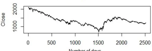
The stock market prices of S&P 500 from 03 March 2005 until 03 March 2015 period of 10 years is used as input for this research. The data was once downloaded from yahoo finance, an open source information provider with 15 minutes delay. The S&P 500 is an American stock index which comprises of 500 corporations whose usual stocks are also listed in NASDAQ. It is among the relied on indices and it could be considered as fine representation American stock Market. The index values are up-to-date for each 15 seconds of the buying and selling sessions. In this paper EOD prices are used for volatility calculations. The information is organized within the form of growing order of their dates. The downloaded data contains columns with date, opening, closing, highest and lowest prices for that distinctive day together with Volume and adjusted closing costs. 10 years of data contained information of2517 rows. The closing prices are very principal in stock markets and peculiarly at the same time in calculating volatility. The closing price of SP 500 for a period of 10 years is shown in Fig. 1.

(3)

ISSN(Online): 2320-9801

ISSN (Print): 2320-9798

International Journal of Innovative Research in Computer

and Communication Engineering

IV. VOLATILITY

General meaning of volatility can be stability; it refers to the uncertainty or risk of the variations in the Stock values from the average stock value. A high value of volatility indicates that a Stock value can rise to maximum value or fall to a minimum value within a short period of time. High Volatility indicates the stock price is not stable and can change at any point rapidly in the opposite direction. Low value of volatility indicates the stock value stays constant with respect to average volatility without any rapid changes. Compare to high volatility value a low volatility is preferred as it guarantees a stable rise or stable fall. Volatility is important because it helps investors to plan their investments ensuring minimum losses.

Volatility is associated with the sample standard deviation of returns over some period of time. It is computed using the following formula:

^₌ _∑ ₍ ₋₎2

eq. (1)

where is the return of an asset over period t and is an average return over T periods.The variance , could also be used as a measure of volatility. But this is lesscommon, because variance and standard deviation are connected by simplerelationship.

The Volatility is calculated from the stock price Sp is only observed during the time when the market is open and the daily financial data are often available in the form of OHLC (open-high-low-close) and Volume Vi. For the trading days i = 0, . . . , N we denote the morning opening price by Oi, the evening closing price by Ci, the daily lowest price by Li and the daily highest price by Hi for that particular day. In this way we have 1OHLC data per day, yearly we can accumulate 260 values. Among OHLC generally Ci is preferred most for the calculation purpose.

V. METHODOLOGY

(4)

ISSN(Online): 2320-9801

ISSN (Print): 2320-9798

International Journal of Innovative Research in Computer

and Communication Engineering

Step 1: Data Acquisition

The Stock market data is downloaded from a trusted source; in this paper S&P 500 indices 10 years data is used as dataset. The data consists of 2517 samples. The end of the day data are considered as the input in this paper.

Step 2: Data Preparation

The data is arranged as per date i.e. 03 March 2005 as the start date and 03 March 2015 as the end date. The data is arranged in the format of Open, High, low, Close and Volume. The data is checked for missing values, correctness and any other redundant values. The data correctness includes checking each day data whether the High price is really high and low price is really low compared to the open and close price of that particular day data.

Step 3: Volatility

The volatility is calculated with the closing price data samples standard deviation of returns over some period of time. This technique is independent and they use historical prices for volatility estimation.

Step 4: Forecasting Volatility

The estimated volatility is used as input for volatility forecasting. Our methodology uses Machine Learning such as naïve Forecast and Neural Networks, time series based techniques such as Arima, Arfima, Bats Forecast, TbatsForecast, BoxCox Forecast, Rand Walk Forecast, Mean Forecast and Holt Winters forecasting techniques. The volatility is forecasted for next 10 days in advance.

Step 5: Results Comparison

Forecasting techniques forecast the volatility for next 10 days. The forecasting accuracy of all the 10 forecasting techniquesare compared in this section. They are compared with error calculation parameters such as ME, RMSE, MAE, MPE, MAPE, MASE and ACF1. The main aim of this research is to find out an accurate forecasting technique.

VI. VOLATILITY FORECASTING

Financial applications, Stock traders require accurate volatility forecasting as stocks trading is huge risk and involve lots of money. The investments on a stock are made based on its volatility. The focus of any research in volatility model is to derive a model which forecasts volatility with at most accuracy. Volatility is a prime topic in Finance, Stocks, Futures and Options. Volatility is important in both long term and short term investments. Volatility measures the risk associated with a stock, higher the volatility the more is the risk and more are the profits and vice versa. Based on the type of investments the traders prefer low volatility and sometimes high volatility. The volatility forecasting is important because knowing the risks in advance traders can plan their investments accordingly.

Forecasting is always associated with risks and in turn risks are associated with profits. In this research we use different machine learning techniques such as Naïve Bayes,Neural Network based techniques time series techniques like ARIMA, ARFIMA, Random Walk forecast, Mean forecast, Holt Winter forecast, Bats and Tbats forecast. The research tries to explore the best forecasting technique among the 10 technique. Neural Networks are best known classification and forecasting techniques, a feed forward architecture based NN are used to forecast volatility. The current trend in research suggests the time series based auto regressive forecasting techniques also yield better results. The research compares the 10 forecasting techniques to find an accurate forecasting technique that can reduce the risks and increase the profits.

A. ARIMA

The Auto Regressive Integrated Moving Average (ARIMA) is generalization of Autoregressive moving average (ARMA) approach. Box and Jenkins developed ARIMA models from ARMA models; hence these models are also referred as Box-Jenkins models. Box and Tiao(1975)[6] proposed the general transfer function for ARIMA.

(5)

ISSN(Online): 2320-9801

ISSN (Print): 2320-9798

International Journal of Innovative Research in Computer

and Communication Engineering

settings are adjusted by numerical vector. The difference between non seasonal Arima and seasonal Arima are the period (frequency) and seasonal allows its function to drift.

B. ARFIMA

Arfima is a modification of Arima model, ARFIMA (p,d,q) model uses two algorithms Hydman – Khandaralgorithm and Raftreyalgorithm to select p,d,q values. The two mentioned algorithms are used to estimate the forecasting modelling parameters. The changes in Arfima compared to Arima are Arfima model combines fractional difference with Arima.

The steps involved in choosing fractional difference parameter are as follows: Step 1: Assume an ARFIMA (2,d,0) model.

Step 2: The data are selected that are fractionally differenced from the estimated d Step 3: ARMA model is selected from the resulting data.

The final ARFIMA (p,d,q) model is estimated for multiple times using fractional difference. Later the estimations are refined using maximum likely hood estimation.

C. NEURAL NETWORKS

Neural networks are dynamic nonlinear modelling techniques that can handle any complex classification and forecasting problems. The current trends are applying Neural Networks for prediction, classification and forecasting problems. The applications of NN’s are Finance, Medicine, Tele-commerce and Data mining. NN have become an integral part of Artificial Intelligence and Machine learning techniques. Neural networks are always used when the exact nature of the inputs and output is not known. The research progress in NN have given a different combination of input, hidden and output layers to handle variety of complex problems.

In this paper we are using Neural Network with Feed-forward architecture designed to have a single hidden layer and inputs are feed with a lag for forecasting volatility. This type of architecture is used for non-seasonal time series data. The numbers of inputs to the Network are decided based on the number of seasonal lags. If the data is in non-seasonal time series format the number of lags are decided based on the optimum number of lags for a linear Auto Regressive model. If the data is of seasonal time series type then above mentioned method is used, with seasonal data set.

D. Naïve Forecast

Naïve forecasts are probably the most rate-strong forecasting model; they are widely used as they provide a benchmark towards which extra sophisticated models. In time series data, making use of naive method would produce forecasted values and last determined values are nearly equal. Naive procedure works quite well for financial and economic time series, which most likely have patterns which can be complex to become aware of and forecast accurately. If the time series is believed to have seasonality, seasonal naive process could also be extra correct the place the forecasts are equal to the worth from last season. The naive method may additionally use a drift, in order to take last observation plus the average change from the first observation to the last observation.

In time series notation: If we let the historical data be denoted by y1,…,yT, then we can write the forecasts as The notation y^T+h|T is a short-hand for the estimate of yT+hbased on the data y1,…,yT.

y^T+h|T = yT eq. (2) y^T+h|T = ∑ (yt – yt-1) eq.(3)

This method is simplest proper for time series data. All forecasts are comfortably set to be the worth of the last observation. The forecasts of all future values are set to be yT, where yT is the final located value. This system works remarkably well for a lot of economic and financial time series.

E. BATS

(6)

ISSN(Online): 2320-9801

ISSN (Print): 2320-9798

International Journal of Innovative Research in Computer

and Communication Engineering

The BATS model is probably the most obvious generalization of the natural seasonal innovations items to enable for a couple of seasonal periods. Nonetheless, it can't accommodate non-integer seasonality, and it might probably have an extraordinarily large quantity of states; the preliminary seasonal factor alone includes mT non-zero states. This turns into a huge number of values for seasonal patterns with excessive periods. BATS Forecasting model are observed to perform better on the short series compared to long series when compared to TBATS forecasting models.

F.TBATS

A new class of innovations state space models is obtained by replacing the seasonalcomponent s(i)t in equation by the trigonometric seasonal formulation, and the measurementequation by

y(ω)t = `t−1 + φbt−1 + ∑ ( ) −1+ dt eq. (4)

This class is designated byTBATS, the initial T denotes “Trigonometric”. To provide more details about their structure,

this identifier is supplemented with relevant arguments to give the designation TBATS(ω,φ, p,q,{m1, k1},{m2, k2},...,{mT , kT}).

A TBATS model requires the estimation of 2(k1 +k2 +•••+kT ) preliminary seasonal values, a number which is more likely to be so much smaller than the number of seasonal seed parameters in a BATS items. In view that it relies on trigonometric features, it can be used to model non-integer seasonal frequencies. A TBATS mannequin should be special from two other related (Proietti 2000) more than one supply of error seasonal formulations offered by using Hannan et al. (1970) and Harvey (1989).

One of the vital key advantages of the TBATS modelling framework are:

(i) it admits a bigger effective parameter house with the possibility of higher forecasts

(ii) it permits for the lodging of nested and non-nested multiple seasonal add-ons

(iii) it handles typical nonlinear aspects that are almost always visible in real time sequence

(iv) it permits for any autocorrelation in the residuals to be taken under consideration

G. BOXCOX Transforms

George Box and Sir David Cox collaborated on one paper (Box, 1964). The Box-Cox transformation of the variable x

is also indexed by λ, and is defined as

xλ’= eq.(5)

Transformations aim at bettering the statistical analysis of time series, by means of discovering a suitable scale for which a model belonging to a easy and well known class, eg. thetraditional regression models, has the excellent performance. A most important type of transformations suitable for time series measured on a ratio scale with strictly confident support is the power transformation; at first proposed by Tukey (1957), as a algorithm for obtaining a model with simple structure, average errors and constant error variance, it was subsequently modified with the aid of Box and Cox (1964).

H. Holt Forecast

Holt-Winters (HW) is the label we almost always supply to a collection of tactics that form the core of the exponential-smoothing loved ones of forecasting ways. The elemental constructions had been supplied by C.C. Holt in 1957 and his student Peter Winters in 1960. Holt (1957) and Winters (1960) accelerated Holt’s approach to capture seasonality. The Holt-Winters seasonal approach contains the forecast equation and three smoothing equations - one for the level ℓt, one for development bt, and one for the seasonal factor denoted by using st, with smoothing parameters α, β∗and γ. We use

m to indicate the interval of the seasonality, i.e., the quantity of seasons in a year. For illustration, for quarterly information m=4, and for monthly knowledge m=12.

(7)

ISSN(Online): 2320-9801

ISSN (Print): 2320-9798

International Journal of Innovative Research in Computer

and Communication Engineering

terms (percentages) and the series is seasonally adjusted via dividing by means of via the seasonal element. Inside each and every year, the seasonal component will sum up to approximately m.

I. Average method

Here, the forecasts of all future values are equal to the mean of the historical data. If we let the historical data be denoted by y1,…,yT, then we can write the forecasts as

y^T+h|T=(y1+⋯+yT)/T eq. (6)

The notation y^T+h|T is a short-hand for the estimate of yT+hbased on the data y1,…,yT.

Despite the fact that we have used time series notation here, this system will also be used for move-sectional data (after we are predicting a price not incorporated within the knowledge set). Then the prediction for values not found is the average of those values which have been determined. The rest ways on this section are simplest applicable to time series knowledge.

J. Random Walk Forecast

A random walk is defined as a process where the current worth of a variable is composed of the past worth plus an error term outlined as a white noise (a natural variable with zero mean and variance one).

Algebraically a random stroll is represented as follows:

yt = yt−1 + t eq. (7)

The implication of a approach of this variety is that the excellent prediction of y for next period is the present value, or in other phrases the procedure does now not permit to predict the change (yt− yt−1). That's, the trade of y is definitely

random. It can be proven that the imply of a random walk procedure is regular but its variance is just not. As a consequence a random stroll process is nonstationary, and its variance raises with t.

In practice, the presence of a random walk system makes the forecast method very simple due to the fact that the entire future values of yt+sfor s > zero, is effectively yt.

VII. RESULTS

The purpose of this research work was to find an accurate volatility forecasting technique. We have used 10 techniques to forecast volatility. Out of 10 results of volatility forecast techniques, one technique will be selected as the accurate technique. The accuracy is measured by six error measuring techniques, all the 10techniques are tested for error measurements and the technique with minimum error is selected as most accurate technique.

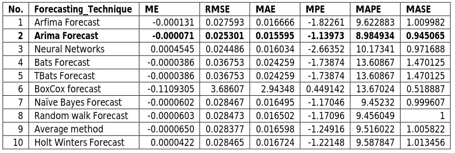
The results of each volatility forecasting technique for six error measuring techniques are tabulated in the tables. The Table.1 contains the forecasting results of all the 10 techniques. The accurate results among the 10 techniques are identified with bold mark. Arima forecasts are more accurate and their error rates are less compared to other techniques. Arima performed better in ME, MAE and MAPE error parameters.

The 6 error measuring parameters used in this research to select an accurate technique are

1. Root Mean Square Error (RMSE) is measure of the differences between values predicted by a trained model

and the actually values.

RMSE = ∑ ( ^₋₎2

eq. (8)

2. Mean Absolute Error (MAE) is an error measuring quantity used to measure the closeness of forecasts and the

actual outcomes.

MAE = ∑ | ^₋ _|_{eq. (9)}

3. Mean Absolute Percentage Error (MAPE) is a measure of prediction accuracy in percentage, it is mainly used

for trend estimation in statistics.

(8)

ISSN(Online): 2320-9801

ISSN (Print): 2320-9798

International Journal of Innovative Research in Computer

and Communication Engineering

4. Mean Error (ME) is measured as average of the errors that occurs due to difference in Actual and predicted

values.

ME = ∑ ( ^₋ ₎_{eq. (11)}

5. Mean Absolute Scaled Error (MASE) is a unique type of forecastthat can be used to compare forecast methods

on a single series as well as for multiple series. MASE =

, eq. (12)

6. Mean Percentage Error (MPE) is the computed average of percentage errors by which forecasts of a model differ from actual values of the quantity being forecast.

MPE = %∑ |

^ _|

eq. (13)

From Table. 1 it is observed that Arima technique had performed better than all the other techniques having least score in error parameters. Hence our research suggests results of Arima forecasting are best compared all other forecasting techniques used in this research.

VIII. CONCLUSION AND FUTURE WORK

The aim of this research work was to forecast volatility with high accuracy. We used SP 500 indices stock market end of the day data for a period of 10 years for volatility forecasting. The volatility was calculated using standard deviation of returns over period of time. The volatility was given as input for 10 forecasting techniques. The volatility was forecasted for 10 days in advance using machine learning techniques such as Naïve Forecast and Neural Network based techniques and time series forecasting techniques such as Arima, Arfima, Bats, Tbats, BoxCox, Rand Walk Forecast, Average method and Holt Winter’s forecast. Among the 10 forecasted results, one highly accurate forecasting technique was selected based on the lowest score in error measuring parameters. Arima forecasting technique has forecasted with high accuracy compared to all other techniques. The future work of this research can be the application of Hybrid techniques to forecast volatility. The Hybrid techniques may involve combining two or more techniques to improve the results.

The Table.1 contains the error rate comparison of the forecasting techniques, results from the result suggest Arima techniques forecasts are more accurate compared to other techniques it is highlighted in bold as shown in the table

Table 1.Error measurement parameters of forecasting techniques

No. Forecasting_Technique ME RMSE MAE MPE MAPE MASE

1 Arfima Forecast -0.000131 0.027593 0.016666 -1.82261 9.622883 1.009982

2 Arima Forecast -0.000071 0.025301 0.015595 -1.13973 8.984934 0.945065

3 Neural Networks 0.0004545 0.024486 0.016034 -2.66352 10.17341 0.971688

4 Bats Forecast -0.0000386 0.036753 0.024259 -1.73874 13.60867 1.470125

5 TBats Forecast -0.0000386 0.036753 0.024259 -1.73874 13.60867 1.470125

6 BoxCox forecast -0.1109305 3.68607 2.94348 0.449142 13.67024 0.518887

7 Naïve Bayes Forecast -0.0000602 0.028467 0.016495 -1.17046 9.45232 0.999607

8 Random walk Forecast -0.0000603 0.028473 0.016502 -1.17096 9.456049 1

9 Average method -0.0000650 0.028377 0.016598 -1.24916 9.516022 1.005822

10 Holt Winters Forecast 0.0000422 0.028465 0.016724 -1.22148 9.587847 1.013456

REFERENCES

[1] TrilochanTripathy, Luis A. Gil-Alana, “Suitability of Volatility Models for Forecasting Stock Market Returns: A Study on the Indian National Stock Exchange”, American Journal of Applied Sciences, 7 (11): 1487-1494, 2010.

[2] Javier Contreras et al. “ARIMA Models to Predict Next-Day Electricity Prices”, IEEE Transactions on Power Systems, Vol. 18, No. 3, Pp. 1014 – 1020, August 2003.

(9)

ISSN(Online): 2320-9801

ISSN (Print): 2320-9798

International Journal of Innovative Research in Computer

and Communication Engineering

[4] Michael W. Brandt et al., “Estimating Historical Volatility”, Online Journal.

[5] Amir Omidi et al., “Forecasting stock prices using financial data mining and Neural Network”, IEEE Transactions, 978-1-61284-840-2/11/2011. [6] B. Uma Devi et al., “An Effective Time Series Analysis for Stock Trend Prediction Using ARIMA Model for Nifty Midcap-50”, International Journal of Data Mining & Knowledge Management Process (IJDKP) Vol.3, No.1, January 2013.

[7] L. Jaresova, “EWMA Historical Volatility Estimators”, ActaUniversitatisCarolinae. MathematicaetPhysica, Vol. 51 (2010), No. 2, 17-28. [8] Dingding Zhou at al., “Network traffic prediction based on ARFIMA model”, IJCSI International Journal of Computer Science Issues, Vol. 9, Issue 6, No 3, November 2012.

[9] Akindynos-NikolaosBaltas et al., “Improving Time-Series Momentum Strategies: The Role of Trading Signals and Volatility Estimators”, Online Journal.

[10] Amine LAHIANI et al., “Testing for threshold effect in ARFIMA models: Application to US unemployment rate data”, Swiss Finance Institute Research Paper Series N°08 – 42

[11] Akram, M., Hyndman, R. & Ord, J. (2009), ‘Exponential smoothing and non-negative data’, Australian and New Zealand Journal of Statistics 51(4), 415–432.

[12] Box, G. E. P. & Cox, D. R. (1964), ‘An analysis of transformations’, Journal of the Royal Statistical Society, Series B 26(2), 211–252.

[13] Hyndman, R. J., Koehler, A. B., Ord, J. K. & Snyder, R. D. (2005), ‘Prediction intervals for exponential smoothing using two new classes of state space models’, Journal ofForecasting 24, 17–37.

BIOGRAPHY

Hemanth Kumar P. is a Ph.D. research scholar in Computer Science & Engineering at Visvesvaraya Technological University, Bangalore. He has completed his M.Tech from Maulana Azad National Institute of Technology, Bhopal and B.E. from Global Academy of Technology, Bangalore. Presently working as Data Scientist atPredictive Research, Bangalore.