ABSTRACT
HSU, CHIA-CHUN. A Genetic Algorithm for Maximum Edge-disjoint Paths Problem and Its Extension to Routing and Wavelength Assignment Problem. (Under the direction of Dr. Shu-Cherng Fang.)
Optimization problems concerning edge-disjoint paths in a given graph have attracted
considerable attention for decades. Lots of applications can be found in the areas of call admission control, real-time communication, VLSI (Very-large-scale integration) layout and
reconfiguration, packing, etc. The optimization problem that seems to lie in the heart of these problems is the maximum edge-disjoint paths problem (MEDP), which is NP-hard. In this dissertation, we developed a novel genetic algorithm (GA) for handling the problem. The
proposed method is compared with the purely random search method, the simple greedy algorithm, the multi-start greedy algorithm, and the ant colony optimization method. The
computational results indicate that the proposed GA method performs better in most of the instances in terms of solution quality and time.
Moreover, a real-world application of the routing and wavelength assignment problem (RWA), which generalizes MEDP in some aspects, has been performed; and the computational results further confirm the effectiveness of our work. Compared with the
bin-packing based algorithms and particle swarm optimization, the proposed method can achieve the best solution on all testing instances. Although it is more time-consuming than
A Genetic Algorithm for Maximum Edge-disjoint Paths Problem and Its Extension to Routing and Wavelength Assignment Problem
by Chia-Chun Hsu
A dissertation submitted to the Graduate Faculty of North Carolina State University
in partial fulfillment of the requirements for the Degree of
Doctor of Philosophy
Industrial Engineering
Raleigh, North Carolina
2013
APPROVED BY:
________________________________ ________________________________
Dr. Shu-Cherng Fang Dr. James R. Wilson
Chair of Advisory Committee
________________________________ ________________________________ Dr. Salah E. Elmaghraby Dr. Yuan-Shin Lee
DEDICATION
This dissertation is dedicated to: God,
my parents Hung-Chi Hsu and Mei-Chiao Peng, my little sister Pei-Wen Hsu,
my girlfriend Kuan-Lin Chen
BIOGRAPHY
ACKNOWLEDGMENTS
TABLE OF CONTENTS
LIST OF TABLES ... viii
LIST OF FIGURES ... ix
Chapter 1 Introduction ... 1
1.1 Problem description ... 2
1.2 The model for maximum edge-disjoint paths problem ... 3
1.3 Importance and applications ... 4
1.4 Difficulties of the maximum edge disjoint paths problem ... 7
1.5 Routing and wavelength assignment problem ... 8
1.5.1 Background ... 8
1.5.2 WDM networks ... 10
1.5.3 Problem description ... 13
1.5.4 Mathematical model of RWA ... 15
1.6 Outline of the dissertation ... 17
Chapter 2 Literature Review ... 19
2.1 A special case: Menger’s Theorem ... 19
2.2 Known approximation ratios for MEDP ... 20
2.3 Existing solution methods for MEDP ... 22
2.3.1 LP relaxation and rounding method ... 22
2.3.2 Greedy algorithms ... 23
2.3.3 Ant-colony optimization ... 27
2.4 Genetic algorithms for path-related problems ... 32
2.4.1 Encoding methods ... 33
2.4.2 Genetic operators ... 37
2.5 Related works on RWA ... 41
2.6 Particle swarm optimization for RWA ... 44
2.6.1 Introduction of PSO ... 44
2.6.2 PSO for RWA ... 46
2.8 Known lower bounds ... 53
Chapter 3 Proposed genetic algorithm for MEDP ... 55
3.1 MEDP with pre-determined paths ... 56
3.2 Encoding/Decoding procedures ... 57
3.3 Initial population ... 61
3.4 Genetic operators ... 63
3.4.1 Crossover Operator ... 64
3.4.2 Mutation Operator ... 66
3.4.3 Self-Adaption Operator ... 67
3.5 Improvement heuristics ... 70
3.6 Fitness function and evaluation ... 73
3.7 Population management and selection method ... 74
3.8 Summary ... 75
Chapter 4 Computational results ... 76
4.1 Design of experiment ... 76
4.2 Problem generation and computational experiments ... 77
4.3 Computational results ... 78
4.3.1 Random search vs. GA ... 79
4.3.2 Greedy algorithms vs. GA ... 82
4.3.3 ACO vs. GA ... 86
4.4 Summary ... 100
Chapter 5 Solving the RWA problem ... 101
5.1 Proposed method ... 101
5.2 An illustration ... 104
5.3 Testing instances and parameter tuning ...110
5.3.1 Testing instances ...110
5.3.2 Tuning the batch size ...115
5.4 Computational experiments ...118
5.4.2 GA_MEDP_RWA vs. PSO ... 127
5.5 Summary ... 130
Chapter 6 Conclusion and future research ... 131
6.1 Summary of work done ... 131
6.2 Future research ... 133
LIST OF TABLES
Table 1 Summary of the performance of the three encoding methods ... 37
Table 2 Main quantitative measures of the instances ... 78
Table 3 Comparison of the results obtained by SGA, MSGA and proposed GA with 3 initial populations ... 84
Table 4 Comparison of the results obtained by MSGA, ACO and the proposed GA with 3 initial populations ... 87
Table 5 The randomly generated connection request set ... 106
Table 6 The updated request set after the first run of GA_MEDP ... 107
Table 7 The updated request set after the backward-scanning process ... 108
Table 8 The updated request set after the second run of and the backward-scanning ... 109
Table 9 The result of applying GA_MEDP_RWA on the small example ...110
Table 10 Main quantitative characteristics of the instances ... 111
Table 11 Testing instances ...113
Table 12 Results of GA_MEDP_RWA and bin-packing based methods (time unit: sec) ...119
LIST OF FIGURES
Figure 1 A WDM transmission system [17]... 12
Figure 2 A wavelength-routed WDM network [17] ... 13
Figure 3 A wavelength-routed network with three lightpaths ... 14
Figure 4 The brick-wall graph ... 22
Figure 5 An example of variable-length chromosome and its decoded path ... 34
Figure 6 An example of fixed-length chromosome and its decoded path ... 35
Figure 7 An example of priority-based chromosome and its decoded path ... 36
Figure 8 An illustration of Order Crossover ... 38
Figure 9 An illustration of Position-based Crossover ... 39
Figure 10 An illustration of Inversion Mutation ... 39
Figure 11 An illustration of Insertion Mutation ... 40
Figure 12 An illustration of Swap Mutation ... 40
Figure 13 The velocity and position updates of a particle in a two-dimensional space ... 46
Figure 14 The structure of a chromosome ... 58
Figure 15 Swap operation generates a new initial individual ... 62
Figure 16 Chromosome 1 and its representing path set ... 65
Figure 17 Chromosome 2 and its representing path set ... 65
Figure 18 The offspring and its representing path set ... 66
Figure 19 The offspring generated by mutation operator ... 67
Figure 20 The offspring generated by self-adaption operator ... 70
Figure 21 Three paths of corresponding requests ... 72
Figure 22 Two EDPs found by GMIN ... 72
Figure 23 A new EDP found by the improvement heuristics ... 73
Figure 24 Evolution of the solution quality obtained by GA and random search on AS-BA.R-Wax.v100e190 with 40 connection requests (upper and lower dot lines denote the boundaries of 95% confidence intervals) ... 81 Figure 25 Evolution of the solution quality obtained by GA and random search on
boundaries of 95% confidence intervals) ... 82 Figure 26 Confidence intervals of the solution quality obtained by three algorithms on
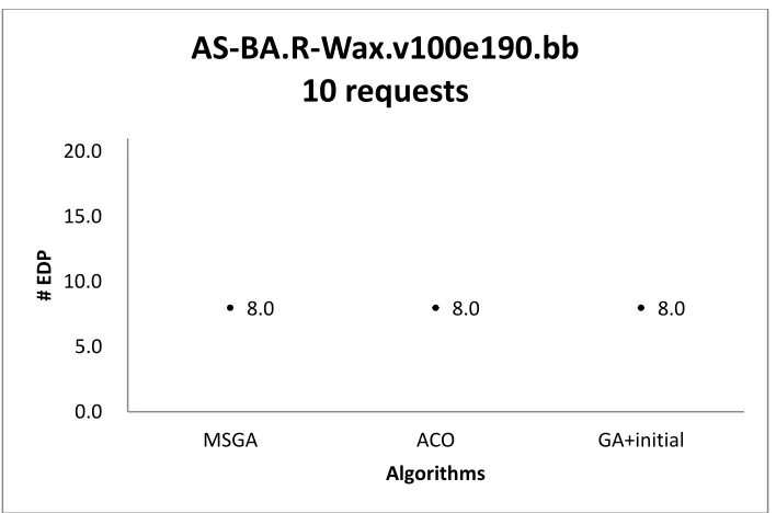
AS-BA.R-Wax.v100e190.bb with 10 requests ... 90 Figure 27 Confidence intervals of the solution quality obtained by three algorithms on
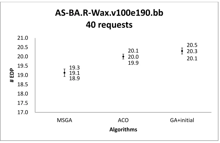
AS-BA.R-Wax.v100e190.bb with 25 requests ... 90 Figure 28 Confidence intervals of the solution quality obtained by three algorithms on
AS-BA.R-Wax.v100e190.bb with 40 requests ... 91 Figure 29 Confidence intervals of the solution quality obtained by three algorithms on
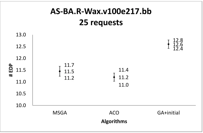
AS-BA.R-Wax.v100e217.bb with 10 requests ... 91 Figure 30 Confidence intervals of the solution quality obtained by three algorithms on
AS-BA.R-Wax.v100e217.bb with 25 requests ... 92 Figure 31 Confidence intervals of the solution quality obtained by three algorithms on
AS-BA.R-Wax.v100e217.bb with 40 requests ... 92 Figure 32 Confidence intervals of the solution quality obtained by three algorithms on
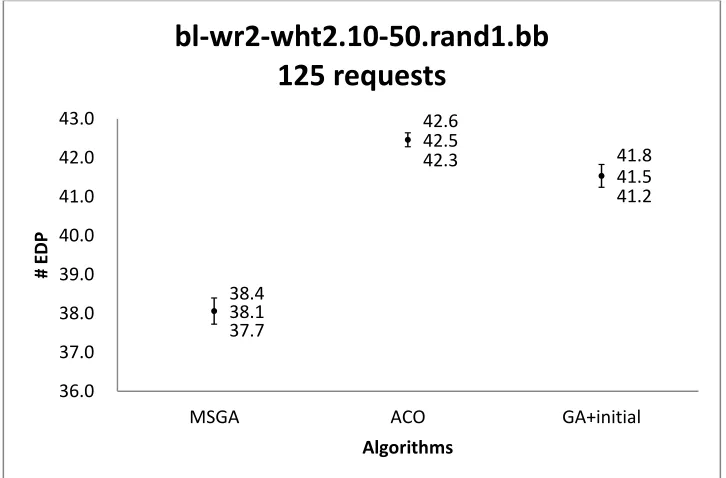
bl-wr2-wht2.10-50.rand1.bb with 50 requests ... 93 Figure 33 Confidence intervals of the solution quality obtained by three algorithms on
bl-wr2-wht2.10-50.rand1.bb with 125 requests ... 93 Figure 34 Confidence intervals of the solution quality obtained by three algorithms on
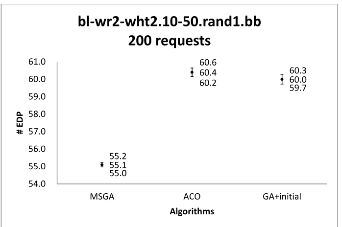
bl-wr2-wht2.10-50.rand1.bb with 200 requests ... 94 Figure 35 Confidence intervals of the solution quality obtained by three algorithms on
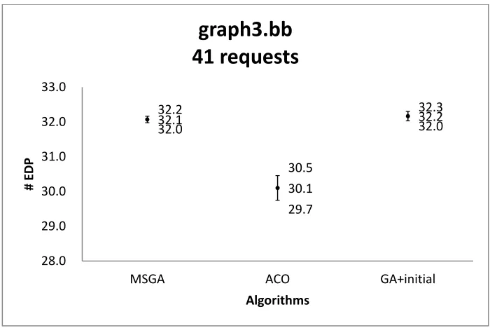
graph3.bb with 16 requests ... 94 Figure 36 Confidence intervals of the solution quality obtained by three algorithms on
graph3.bb with 41 requests ... 95 Figure 37 Confidence intervals of the solution quality obtained by three algorithms on
graph3.bb with 65 requests ... 95 Figure 38 Confidence intervals of the solution quality obtained by three algorithms on
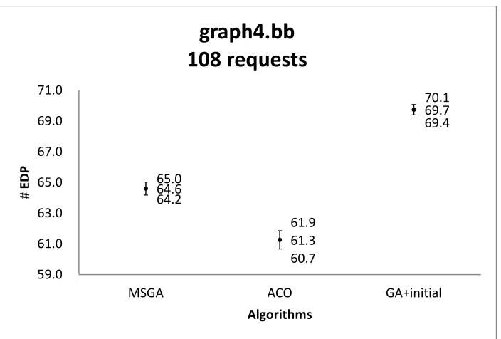
graph4.bb with 43 requests ... 96 Figure 39 Confidence intervals of the solution quality obtained by three algorithms on
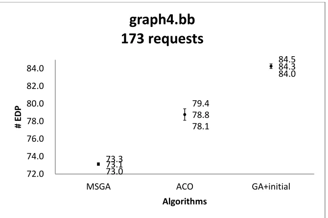
Figure 40 Confidence intervals of the solution quality obtained by three algorithms on
graph4.bb with 173 requests ... 97
Figure 41 Confidence intervals of the solution quality obtained by three algorithms on mesh10X10 with 10 requests ... 97
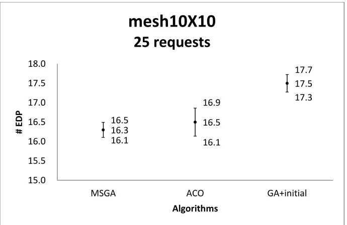
Figure 42 Confidence intervals of the solution quality obtained by three algorithms on mesh10X10 with 25 requests ... 98
Figure 43 Confidence intervals of the solution quality obtained by three algorithms on mesh10X10 with 40 requests ... 98
Figure 44 Confidence intervals of the solution quality obtained by three algorithms on mesh15X15 with 23 requests ... 99
Figure 45 Confidence intervals of the solution quality obtained by three algorithms on mesh15X15 with 57 requests ... 99
Figure 46 Confidence intervals of the solution quality obtained by three algorithms on mesh15X15 with 90 requests ... 100
Figure 47 Illustration of NSF network with 16 nodes and 25 edges ... 105
Figure 48 95% C. I. of the objective value obtained with different on janos-us-ca_08 ...116
Figure 49 95% C. I. of the computational time with different on janos-us-ca_08 ...116
Figure 50 95% C. I. of the objective value obtained with different on USAnet_08 ...117
Figure 51 95% C. I. of the computational time with different on USAnet_08 ...117
Figure 52 Number of times that the best value is achieved by different methods among 67 instances ... 122
Figure 53 Number of times that the worst value is achieved by different methods among 67 instances ... 122
Figure 54 Relative difference of computational time on graph “Norway” ... 124
Figure 55 Relative difference of computational time on graph “giul” ... 124
Figure 56 Relative difference of computational time on graph “Germany” ... 125
Chapter 1
Introduction
Assigning paths to connection requests is one of the basic operations in the modern communication networks. Each connection request is a pair of physically separated nodes
that require a path for information transmission. Given such a set of connection requests, due to the capacity restrictions, one may want to assign paths to requests in such a way that no
two paths share an edge in common. These paths are called edge disjoint paths (EDPs). A natural question to ask is: What is the maximum number of requests that are simultaneously realizable as edge disjoint paths? This is called the maximum edge-disjoint paths (MEDP)
problem, which turns out to be one of the classical combinatorial problems in the NP-complete category. It has been extensively studied for decades and can be extended to
many real-world applications, e.g., the routing and wavelength assignment (RWA) problem, the call admission problem, the unsplittable flow problem, and the very large-scale integration (VLSI) problem, etc. In this dissertation, we propose a novel genetic-based
algorithm to solve the MEDP problem. Moreover, the proposed algorithm is extended for solving the RWA problem. Computational results show that in either case, the proposed
method exhibits good performance compared with other existing solution methods.
This chapter intends to introduce some background information on the problems we are going to tackle. The first four sections provide the descriptions, formulation, importance and
difficulties of the MEDP problem, respectively. Then an overview and background information on the RWA problem is given in Section 1.5. Following that is an outline of the
1.1
Problem Description
The physical architecture of the network is given in the form of an undirected and connected
graph , which consists of a finite set of vertices and a finite set of edges,
where and . Each edge is said to be incident to and to
, and are called endpoints of . A sequence of edges such that
for some , is called a path of length , with endpoints
and . We say that two paths are edge-disjoint (or edge-independent) if they do not have
any edge in common. A set of paths is said to consist of edge-disjoint paths (EDPs) if any two paths in the set are edge-disjoint.
Let be a set of connection requests.
Each request in a graph is a pair of vertices that asks for a path that establishes
the connection between and . We often use “request ” and “request ”
interchangeably.
An instance of the maximum edge-disjoint paths (MEDP) problem consists of an undirected graph and a request set . A feasible solution of MEDP is
given by a subset , such that each request in is assigned a path. The assigned paths
are pairwise edge-disjoint and denoted by . More precisely, a path between and
is assigned to each such that no two paths , ( ) have
an edge of the graph in common. The goal of the maximum edge-disjoint paths problem is to
maximize the cardinality of . The requests in are called realizable (or accepted) requests,
Problem: maximum edge-disjoint paths (MEDP) problem.
Input: undirected graph , connection requests
.
Feasible Solution: a realizable subset such that there is an assignment of edge-disjoint paths to the requests in .
Goal: maximize .
1.2
The Integer Linear Programming Model for Maximum
Edge-disjoint Paths Problem
MEDP has a natural IP formulation based on multicommodity flows. We use an
exponentially sized path formulation for convenience. The notations of the MEDP model are defined as follows:
the set of all simple (cycle-free) paths in from to , for .
: the set of all simple (cycle-free) paths in that pass along edge .
: a binary variable indicating whether path is chosen in the solution, for each
.
: a binary variable indicating whether the request is realizable, for . The formulation of MEDP is the following linear integer program:
(1.1)
, (1.3)
(1.4)
(1.5)
The objective function (1.1) maximizes the number of realizable connection requests. Constraint (1.2) ensures that each realizable request is assigned a path. Constraint (1.3) ensures that each edge can only be used by at most one path. Constraints (1.4) and (1.5)
ensure that all variables are binary.
Enumerating all possible simple paths for each of the connection requests makes solving
the model extremely time consuming. Considering the case on a complete graph (in which every pair of distinct vertices is connected by an unique edge), the number of all-possible simple paths that connects a pair of node is
, where .
For instance, in a complete graph which has 10 nodes, enumerating all possible simple
paths for a pair of nodes has order of time complexity. Thus solving this integer linear
programming model is not an efficient way for tackling the MEDP problem.
1.3
Importance and applications
the modern high-speed communication networks has brought more focus to the MEDP problem [11]. Many modern network architectures establish a virtual path between any two
vertices. In order to achieve guaranteed service quality, the network must reserve sufficient resources (capacity or bandwidth) on the edges along that path. Some requests are rejected if
the path does not have sufficient capacity. We want to know how many requests are realizable in a round using edge-disjoint paths, and how many rounds of communication are required to satisfy all requests. The MEDP problem is the essence of these types of problems.
In the real world, the maximum edge-disjoint paths problem has a multitude of applications in the areas of call admission control [37, 38], real-time communication, VLSI
(very-large-scale integration) layout [3] and reconfiguration [42], packing [1, 30, 31], etc. In addition, the routing and wavelength assignment (RWA) problem [2, 11, 27], unsplittable flow problem (UFP) [14, 30, 33, 39], and the call admission problem [37, 38] are direct
extensions of MEDP. These real-world applications of the maximum edge-disjoint paths problem generalize the original MEDP in one or more aspects. In fact, MEDP is essentially in
the heart of several network optimization problems and therefore, its importance is significant. The three classical applications of MEDP are further introduced below.
The routing and wavelength assignment (RWA) problem
Optical networks that apply the wavelength division multiplexing (WDM) technology have attracted enormous attention due to its capability of satisfying the increasing capacity
lightpath, which can be characterized by its route and the assigned wavelength.
Given an optical network and a set of lightpath requests, the routing and wavelength
assignment (RWA) problem attempts to route and assign a wavelength to each lightpath request subject to the following constraints: (a) wavelength continuity constraint: the same
wavelength must be assigned to the entire route if there are no available wavelength converters; and (b) wavelength clash constraint: two lightpaths sharing the same edge have to use different wavelengths.
The objectives of RWA include the minimization of the required number of wavelengths to satisfy all lightpath requests, or maximization of the number of realizable lightpath
requests subject to a given number of wavelengths. In later chapters, more details including problem background and related works will be further introduced.
The unsplittable flow problem (UFP)
The unsplittable flow problem is one of the most extensively studied optimization problems in the field of networking [14, 30, 33, 39]. It is essentially a generalization of MEDP in
several aspects. For a given undirected graph , each edge now has a capacity
. With respect to the set of connection requests , each request has a demand and
a profit , assuming that the edge capacities, demands and profits are positive real numbers.
A feasible solution is given by selecting a subset of requests and assigning a path from to
for each realizable request , subject to the following constraints: (i) for an edge , the
sum of demands of all the accepted requests that pass through cannot exceed the capacity
; (ii) for an accepted request , it must send units of demand through a single route.
It is easy to see that MEDP is a special case of UFP in which for every ,
and for every request .
Call admission control problem
The call admission control problem is a vital optimization problem encountered in the operations of communication networks [37, 38]. Given an undirected graph and a set of
connection requests, each request has a certain bandwidth requirement and time specification of its starting time and duration. If a request is accepted, then a path has to be routed between the pair of nodes and the required amount of bandwidth is reserved on all links along that
path during the time period.
In addition, each call is associated with some profits, which the network provider will
gain if the desired connection is established. The goal is to maximize the total profits obtained from the accepted requests without violating the edge capacity constraints at any time.
1.4
Difficulties of the maximum edge disjoint paths problem
Most of the early works on the edge-disjoint paths problem have focused on the version of a decision problem, which determines either all the connection requests can be realizable by edge-disjoint paths or certifies that such a routing does not exist. This decision problem is
one of the classical NP-complete problems [1, 24]. Substantial efforts have been made to the identification of polynomial solvable cases for the decision problem, we refer to the surveys
by Frank [3] and Vygen [16] for more details.
Some classes of graphs are able to be checked whether all requests are realizable in polynomial time, but if the answer is no, it is NP-hard to compute the maximum number of
realizable requests. Reference [33] provides some examples. Since MEDP is an NP-hard problem on general graphs [39], many studies were devoted to obtaining good approximation
algorithms and exploring more tractable classes. For instance, MEDP on chains can be solved in polynomial time since the routing for each request in a chain is uniquely determined by its endpoint (this fact also holds for arbitrary trees). Hence, the connection requests can be
treated as a set of intervals on the real line and the problem of finding a maximum number of disjoint intervals is known to be solvable in linear time. We refer to the survey in [33] for
more details and other tractable graphs (e.g., bidirected chains, undirected trees, bidirected stars).
1.5
Routing and wavelength assignment problem
In recent decades, the number of bandwidth-intensive applications in telecommunications
such as HD video, video conferencing, HD digital broadcasting and streaming over the internet, have grown rapidly. The technology of fiber-optics can be an attractive candidate for
meeting the above-mentioned needs because of its huge transmission bandwidth (~50 Tbps), low signal attenuation, low signal distortion, low power requirement, small space
requirement, and low cost. This section starts with the background of optical fibers and WDM networks, and then gives a precise description of the routing and wavelength problem.
1.5.1
Background
attenuation low enough for communication purposes. In the meanwhile, GaAs semiconductor lasers were developed, which were suitable for transmitting light through optical cables for
long distances. Starting from 1975, the first commercial fiber-optics communications system was developed, and it operated at a bit rate of 45 Mbps with repeater spacing up to 10 km.
The second generation of fiber-optics communication was developed for commercial use in the early 1980s. By 1987, these systems were operating at bit rates up to 1.7 Gbps with repeater spacing up to 50 km.
Later, scientists developed dispersion-shifted fibers which allowed the third-generation fiber-optics systems operating commercially at a bit rate of 2.5 Gbps with repeater spacing in
excess of 100 km. Finally, the fourth generation of fiber-optics communication systems used optical amplification to reduce the need for repeaters and wavelength-division multiplexing to increase data capacity. These two technologies improved the system capacity dramatically
since 1992. By 2001, such systems operated at a bit rate of 10 Tbps. Finally, a bit-rate of 14 Tbps was reached over a single 160 km line using optical amplifiers in 2006.
In telecommunications or computer networks, multiplexing is a method to combine multiple analog message or digital data streams into one signal over one shared medium. The use of such a technique can further increase the capacity of optical fibers. Four main types of
multiplexing are available: (a) space-division multiplexing (SDM); (b) time-division multiplexing (TDM); (c) code-division multiplexing (CDM); and (d) frequency-division (or
wavelength-division) multiplexing (FDM).
For TDM, two or more bit streams or signals are transferred as sub-channels in one communication channel, but are physically taking turns on the channel. The time domain is
divided into several recurrent time slots of fixed length, one for each sub-channel. The optical TDM bit rate is the aggregate rate over all channels in the system. A disadvantage of
TDM is that it requires that each node has to be perfectly synchronized to the same time clock and be capable of handling the aggregate bit rate of all channels. On the other hand, CDM assigns a code to each transmission and also requires the source and destination nodes
to synchronize to the same time base.
FDM combines several digital signals into one medium by sending signals in several
distinct frequencies over that medium. One of the most common applications is cable television. Only one cable reaches a customer's home but the service provider can send multiple television channels or signals simultaneously over that cable to all subscribers.
Receivers must tune to the appropriate frequency (channel) to access the desired signal. Wavelength-division multiplexing (WDM) is a variant technology used in optical
communications. Since wavelength and frequency are tied together through a simple directly inverse relationship, the two terms actually describe the same concept. WDM operates by dividing the optical transmission spectrum into many non-overlapping wavelengths and each
wavelength supports one communication channel. It allows multiple channels to coexist on a single fiber and does not require nodes to synchronize to the same time clock. Hence WDM
has become the favorite multiplexing technique for optical networks.
1.5.2
WDM networks
optical carrier signals onto a single optical fiber by using different wavelengths (i.e. colours) of laser light. The number of wavelengths that each fiber can carry simultaneously is limited
by the physical characteristics of fibers and the optical technology of combining the wavelengths and separating them off. In early WDM systems, each fiber could only provide
two channels. Modern systems can handle up to 370 signals and can thus expand a basic 273 Gbps system over a single fiber pair to a bit rate over 101Tbps.
Figure 1 [17] is a block diagram of a basic WDM transmission system. The transmitter
comprises a laser and a modulator. The laser is the light source, which generates an optical carrier signal at either a fixed or a tunable wavelength. The carried signal is modulated by an
electronic signal and is sent to the multiplexer (MUX). The multiplexer combines several
optical signals on different wavelengths (denoted by in Figure 1) into a single optical signal, which is transmitted to a common output port or optical fiber. The
network medium can be a simple fiber link, a passive star coupler, or any type of optical network. The demultiplexer (DMUX) uses optical filters to separate the received optical signal into multiple optical signals on different wavelengths, which are then sent to the
receivers. The receiver has a detector that can convert an optical signal to an electronic signal. Optical amplifiers are used at appropriate locations in the transmission system to maintain
Figure 1 A WDM transmission system [17]
A wavelength-routed optical WDM network typically consists of routing nodes interconnected by WDM fiber links in an arbitrary physical topology. Each routing node
employs several transmitters and receivers for transmitting signals to and receiving signals from fiber links, respectively. Each link operates in WDM and supports a certain number of optical channels (or wavelengths). A routing node can be connected to an access node, which
is an interface between the optical network and the electronic client networks. An access node performs traffic aggregation and E/O conversion functions on the source side. On the
destination side, traffic deaggregation and O/E conversion are performed. The architecture of a wavelength-routed WDM network is shown in Figure 2 [17]. In the remainder of this work, we assume that each routing node is connected to an access node, and we refer to this
Figure 2 A wavelength-routed WDM network [17]
1.5.3
Problem description
In a wavelength-routed WDM network, end users communicate with each other via
all-optical WDM-channels, which are referred to as lightpaths. A lightpath is used to establish a connection between two nodes, and it can be characterized by its route and the occupied wavelength. In the absence of wavelength converters, a lightpath must use the same
wavelength on all fiber links which it traverses, which is known as the wavelength continuity constraint. In addition, lightpaths that share a common physical link cannot use the same
wavelength, which is known as the wavelength clash constraint. Figure 3 illustrates a
Figure 3 A wavelength-routed network with three lightpaths
Given a set of connection requests, the problem of setting up lightpaths by routing and
allocating a wavelength to each connection is called the routing and wavelength assignment (RWA) problem. In general, connection requests are of three types: static, incremental and
dynamic. We only consider the static case, which means the entire set of connection requests is known in advance. The routing and wavelength assignment operations are performed off-line.
The RWA problem is to establish routes and assign wavelengths for the connections while minimizing network resources such as the number of wavelengths or the number of
fibers in the network. Alternatively, one may attempt to connect as many requests as possible for a given number of wavelengths. In this work, we consider the former case assuming that
To be precise, given an undirected graph in which each edge is an
optical fiber link in the physical network, and a request set
, the routing and wavelength assignment (RWA) problem searches for a
set of lightpaths in , each corresponds to one request , and
assigns a set of wavelengths to these paths. Path and , ,
cannot be assigned the same wavelength if they share a common edge. The objective is to
minimize the number of wavelengths required to satisfy all requests in .
A feasible solution to the RWA problem consists of a path set and the assigned
wavelength set . Each path connects the request and is assigned the
wavelength such that the wavelength clash constraints hold. The RWA problem can
be stated in a compact way as follows:
Problem: routing and wavelength assignment (RWA) problem.
Input: undirected graph and a set of connection requests
.
Feasible Solution: a path set to connect all requests and a corresponding wavelength set such that the wavelength clash constraint holds.
Goal: minimize the number of required wavelengths.
1.5.4
Mathematical model of RWA
In reference [2], the RWA problem is formulated as an integer linear programming problem
available wavelengths is limited and the goal of their model is to maximize the number of
accepted requests. In our work, we assume there are units of available wavelengths ( is the number of requests). Thus in the worst case, where each wavelength is assigned to
exactly one request, all connection requests can still be satisfied. The goal of our model is to minimize the number of utilized wavelengths to satisfy all requests. Some notations are
defined below.
L: set of indices of available wavelengths (on each edge), .
: a binary variable, if wavelength is assigned to path ; and
otherwise.
: the set of all simple (cycle-free) paths in from source to terminal , for
.
: the set of all simple paths in that pass along edge .
: a binary variable, if wavelength is utilized; and otherwise.
The problem formulation is given by
(1.6)
Subject to
, (1.7)
(1.8)
(1.9)
is the wavelength clash constraint, that is, for the paths in , the wavelength is assigned
to at most one of them. In other words, paths using the same edge must employ different wavelengths. Constraint (1.8) represents the demand constraint, which ensures each request
is assigned exactly a path and a wavelength. Constraint (1.9) ensures will equal 1 if
wavelength is used by one or more paths.
As mentioned in Section 1.2, enumerating all-possible paths is extremely
time-consuming and only applicable in very small-sized networks. The number of
all-possible paths that connect a pair of nodes in a complete graph is . Thus it is
unlikely to tackle the RWA problem by solving the above integer linear programming due to its rapidly increasing number of variables and constraints.
1.6
Outline of the dissertation
The dissertation is organized as following: Chapter 2 includes two parts. The first part is the literature review of the MEDP problem, where some known approximation ratios, existing methods and genetic algorithms for path-related problems are reviewed. The second part is a
survey of the RWA problem, where the background, related works, two existing methods and lower bounds of the problem are provided. In Chapter 3, we propose a novel genetic
algorithm for solving the MEDP problem, including the encoding/decoding scheme, a method to produce the initial population, a fitness function, three reproduction operators, an improvement heuristic, and the population management method. The testing instances and
which employs the proposed GA-based method to solve the RWA problem. The computational results show that the proposed methods outperform the bin-packing based
Chapter 2
Literature Review
In this chapter, we provide a review of the maximum edge-disjoint paths problem (MEDP)
and one of its extended real-world applications – routing and wavelength assignment problem (RWA). In Section 2.1, a special case of MEDP known as edge-disjoint Menger
problem, in which all connection requests are composed by repetitions of the same pair ,
is discussed. Section 2.2 summarizes the approximation ratios of most well-known approximation algorithms for MEDP on a general graph. Detailed descriptions of these
approximation algorithms are given in Section 2.3. In Section 2.4, some encoding schemes and genetic operators for solving path-related problems are introduced. Related works on the
RWA problem are reviewed in Section 2.5, particle swarm optimization (PSO) and the state-of-art bin-packing based methods are given in Sections 2.6 and 2.7, respectively. Finally, lower bounds of solving the RWA problem are provided in Section 2.8.
2.1
A special case: Menger’s Theorem
One extreme case of MEDP is that all of the pairs of connection requests are the same, i.e.,
all requests are between two vertices . In this case, the number of edge-disjoint paths can be viewed as a measurement of how well a given pair of vertices is connected. A
different way of measuring the connectivity is to determine the smallest number of edges whose deletion from the graph disconnects every path between the pair. In 1927, Karl Menger [19] proved an elegant theorem, which states that the maximum number of
minimum number of edges whose deletion disconnects the pair.
To be more precise, given in graph , let set be a collection of edges. We
say is an “ edge-separating set” if every path contains an edge of . We
denote the minimum cardinality of an edge-separating set by and the
maximum number of edge-disjoint paths in by . Since each edge-disjoint
path must contain at least one edge in the edge-separating set, we have
. Menger further proved that in his theorem.
Theorem 1 (Karl Menger, 1927) In an undirected graph , if vertices and are not adjacent, .
2.2
Known approximation ratios for MEDP
Since the maximum edge-disjoint paths problem with connection requests on a general graph is proven to be NP-hard, many works have proposed approximation algorithms for solving
the problem [1, 8, 14, 20, 23, 30, 31, 32, 33]. A good approximation algorithm runs in polynomial time to reach a solution guaranteed to be close enough to the optimal solution.
The sense of “closeness’’ can be described by the “approximation ratio” .
A -approximation algorithm for MEDP runs in polynomial time to output a feasible solution
R satisfying , where OPT is the optimal objective value and is the approximation ratio.
For a general graph, known approximation algorithms for MEDP include the simple greedy algorithm, bounded greedy algorithm and shortest-path first greedy algorithm can be
the detailed descriptions of each algorithm will be given in Section 2.3.
Theorem 2 (Erlebach, 2006 [33]) The simple greedy algorithm has an approximation ratio of for MEDP in a directed or undirected graph with vertices, and the bound
is tight.
Theorem 3 (Kleinberg, 1996 [14]) The bounded greedy algorithm with a parameter
has an approximation ratio of for MEDP in a directed or
undirected graph with edges.
Chekuri and Khanna [8] showed that for MEDP, the shortest-path-first greedy algorithm
gives an approximation for undirected graphs and an approximation for
directed graphs. In the same article, an approximation algorithm was also
shown for acylic graphs. In Varadarajan and Venkataraman’s work [20], the approximation
ratio for directed graphs was improved to . The next theorem provides the
best known approximation ratio for MEDP in terms of the number of vertices.
Theorem 4 (Chekuri and Khanna, 2003 [8]; Varadarajan and Venkataraman, 2004 [20]) The shortest-path-first greedy algorithm for MEDP achieves an approximation ratio of
for undirected graphs and for directed
graphs.
Lastly, an essential inapproximabilty result for directed graphs has been obtained by Guruswami et al. [39].
Theorem 5 (Guruswami et al., 1999 [39]) For MEDP in a directed graph with edges, there cannot be an -approximation algorithm for any unless .
2.3
Existing solution methods for MEDP
Known solution methods for the MEDP include the “LP relaxation and rounding” method,
the “greedy algorithms”, and the “Ant Colony Optimization” approaches, which are presented in this section.
2.3.1
LP relaxation and rounding method
The formulation of MEDP shown in Section 1.2 is an integer linear program whose complexity grows exponentially in terms of the problem size. Relaxing (1.4) and (1.5) by
and respectively, leads to an LP relaxation such that an optimal
fractional solution can be acquired in polynomial time. Then the rounding techniques are applied to covert the fractional solution into an integral solution. However, the gap between the fractional optimum and integral optimum can be large. A brick-wall graph shown in
Figure 4 is a simple example demonstrating this phenomenon.
Assume there are six connection requests {(1,1), (2,2), (3,3), (4,4), (5,5), (6,6)} in Figure 4. When the capacity of each edge is 1, any two paths interfere with each other. We can easily
see that only 1 request is realizable. However, solving the LP relaxation will obtain an objective value of 3, since it routes 0.5 of each request without violating any constraint. This
shows that the fractional solution obtained by using the LP relaxation cannot guarantee much about the original problem. The rounding approach may result in an integral solution far away from desired. However, the situation becomes better as the edge capacity increases. We
refer to reference [33] for more details.
2.3.2
Greedy algorithms
A greedy algorithm starts with an empty solution set and constructs a feasible solution step by step utilizing a greedy strategy. Due to its ease and speed in execution, a greedy algorithm is usually implemented for on-line real practice. In this case, the requests are presented one
by one and the algorithm has to accept or reject the request sequentially without knowing future requests.
The pseudocode of the simple greedy algorithm (SGA) for MEDP is given in Algorithm
1. It starts with empty sets and , then iteratively assigns a shortest path, if there is one, to a connection request following the order that the request set is given. Each time a path is
assigned, all the edges along that path are removed from the graph. The algorithm halts after iterations. Unfortunately, SGA does not achieve a good approximation ratio in general. The
Algorithm 1 Simple Greedy Algorithm (SGA)
Input: and Begin:
1. ; 2. for
3. if then
4. ; 5. ;
6. ; 7. ; 8. end if
9. end for End
Output: Realizable requests R and edge-disjoint paths S
It is easy to see that the solution quality of SGA highly depends on the order of
connection requests. In the worst case, SGA may route the first request on a very long path that interferes with all other requests. This is the main drawback of SGA. An intuitive way to solve this problem is applying the multi-start simple greedy (MSGA) algorithm [23], shown
in Algorithm 2. MSGA runs SGA for times, in each iteration the order of connection requests is randomly regenerated. The algorithm then outputs the best solution of the
Algorithm 2 Multi-start simple greedy algorithm (MSGA)
Input: and , where is the number of restarts Begin:
1. ;
2. ;
3. for
4. ;
5. if then
6. ;
7. ;
8. end if
9. random permutation of ;
10. ; 11. end for
End
Output: Realizable requests and edge-disjoint paths
Another improved greedy algorithm is the bounded-length greedy algorithm shown in
Algorithm 3, proposed by Kleinberg [14]. It takes an extra parameter to denote the threshold of route length. A request is accepted only if it can be routed on a path of length at
most . In other words, requests whose endpoints are at distance larger than will be
rejected. The algorithm has an approximation ratio of if every request can only be routed
with length at least . If this happens, the algorithm will increase by one and run
again. Kleinberg proved that the bounded-length greedy algorithm with parameter
can achieve an approximation ratio of for MEDP in a directed or
Algorithm 3 Bounded-length Greedy Algorithm (BGA)
Input: , and Begin
1. do
2. ; 3. for
4. ;
5. if and then 6. ;
7. ; 8. ; 9. end if
10. end for 11. ; 12. while End
Output: Realizable requests R and edge-disjoint paths S
A further modification of the greedy algorithm is the shortest-path-first greedy algorithm
proposed by Kolliopoulos and Stein [30, 31], shown in Algorithm 4. First, the algorithm acquires the shortest path for each connection request. The request that has the path with the
shortest length among all paths is accepted and removed from the request set. Then the algorithm repeats the same “greedy” strategy until no path can be found for all remaining requests. Obviously, the algorithm accepts requests in a non-decreasing order of the path
length. It has been shown that the worst-case approximation ratio of Algorithm 4 is at least as good as that of bounded greedy algorithm. Kolliopoulos and Stein [30, 31] proved that the
algorithm achieves an approximation ratio of in a directed or undirected graph with
Algorithm 4 Shortest-path-first Greedy Algorithm
Input: and Begin:
1. ;
2. While contains a request that can be routed in
3. a request in such that its shortest path has minimum length among all requests
in ;
4. ;
5. ;
6.
7. ;
8. end while
End
Output: Realizable requests R and edge-disjoint paths S
2.3.3
Ant-colony optimizationn
Ant colony optimization (ACO) was initially proposed by Marco Dorigo in 1992 in his PhD dissertation [21]. The idea of ACO comes from observing the exploitation of food resources
by ants. In the beginning, ants wander randomly. If an ant finds food, it leaves pheromone on the trail back to the colony. Other ants are likely to follow the trail instead of keep travelling
at random. If one eventually finds food, it also leaves pheromone to reinforce the path. On the other hand, the pheromone on paths evaporates gradually, thus reducing its strength of attraction. The pheromone density becomes higher on the shorter paths than the longer ones,
therefore a shortest path between the food source and the ants’ nest may be found eventually. The application of ant colony optimization (ACO) to solving MEDP is the only known
metaheuristic method. In [23], MEDP is decomposed into subproblems .
by an ant. In other words, ants are assigned for the connection requests.
A constructed ant solution contains paths which are not necessarily edge-disjoint.
An edge-disjoint solution is generated by iteratively removing the path that has the most edges in common with other paths, until the remaining paths are mutually edge-disjoint. Let
denote the number of edge-disjoint paths obtained from . Since two
solutions and may have the same number of EDPs, i.e., , a second
criterion is introduced to quantify the non-disjointness of an ant solution. Define as
follows:
, (2.1)
For an ACO intermediate solution , measures the usage of edges that are
covered by more than one path. That means is zero if all paths are mutually
edge-disjoint. Generally speaking, a decrease of may imply an increase of the
number of EDP. Thus we can define an ordering as follows: For two ACO intermediate
solutions and , we say that if and only if
, (2.2)
Or
The pheromone model is critical for the ant colony optimization approach. Since the
subproblem . Each pheromone model consists of a pheromone value for each edge
. All pheromone values are in the range , where and are
user-defined parameters. We denote the set of pheromone models by . Algorithm 5 carries the pseudocode of a basic ACO algorithm. The procedure
sets all the initial pheromone values to be value . In
each iteration, ant solutions are constructed by applying the function
times (with ants), where is a permutation of
. During the process of path construction, an ant iteratively moves from one node
to another along an available edge, the choice of destination can be made either
deterministically or stochastically. We randomly draw a number between 0 and 1. If
, the next step destination is chosen deterministically. Otherwise, the choice is
made stochastically.
After paths are constructed, the value of the variable will be updated if the
solution improves. Finally, the pheromone values are updated depending on the edges
included in . We refer readers to [23] for the details of the path construction and
Algorithm 5 Basic ACO Algorithm
Input: Begin:
1. ;
2. ; 3. while termination condition is false 4. (1,2…,);
5. for
6. ;
7. for
8. h ;
9. ;
10. end for
11. random permutation of ; 12. end for
13. Choose such that
14. if then
15. ;
16. h ; 17. end if
18. end while End
Output: Realizable requests and disjoint paths generated from
In [23], the author also proposed an enriched version of ACO for MEDP. The following four features are added to modify the way of exploring the solution space.
Sequential versus parallel solution construction: While constructing an ACO solution,
backtracking move. This feature changes the dynamics of the searching process that may lead to different results.
Candidate list strategy: This is a mechanism to restrict the number of available choices
for consideration at each construction step. For instance, when applying ACO to the traveling
salesman problem, a restriction on checking a few nearby nodes only may significantly improve the solution efficiency and quality. The modified ACO for MEDP considers only “good” choices at each construction step to speed up the process.
Different search phases: The pheromone update scheme is an important component of
ACO. In the basic algorithm, all the paths (including the non-disjoint paths) of the ant
solution are used for updating the pheromone values. The author of [23] proposed a
two-phase scheme. In the first phase, only the edge-disjoint paths are used for updating the
pheromone values. The second phase kicks in when no improvement can be found over a certain period of time by using all paths to update pheromone values. Once the second phase results in any improvement, the algorithm returns to using the first phase.
Partial destruction of solutions: This mechanism helps the algorithm escape from the
local solutions by removing and reconstructing some paths of the solution. This procedure is
initiated once the algorithm fails to improve over a certain period of time.
In general, ACO approach has advantages over MSGA in terms of solution quality as well as computational time. The details of comparison on several benchmark instances can be
2.4
Genetic algorithms for path-related problems
The genetic algorithm (GA) is a stochastic search method for optimization problems. It
mimics the natural evolution processes using crossover, mutation and selection mechanisms
to gradually improve the solution. Let denote a population set of individuals in
generation and the set of offspring generated by genetic operators. A general structure of the genetic algorithm is given below.
Genetic Algorithm
Begin: 1. ;
2. initialize ; 3. evaluate ;
4. while (terminal condition not met) do 5. recombine to yield ; 6. evaluate ;
7. select from and ; 8. ;
9. End End
Since MEDP considers the paths between several terminal pairs, we review the application of genetic algorithms for the shortest path problem in this section. The shortest
path problem is to find a path between two nodes such that the path length is minimized. It is a fundamental problem involved in many applications on transportation, routing, and
path problem. The encoding schemes and genetic operators are summarized below.
2.4.1
Encoding methods
A gene in a chromosome is characterized by two factors: “locus” denotes the position of the gene within the structure of the chromosome, and “allele” represents the value of the gene. In
[22], three different encoding schemes are investigated:
Variable-Length encoding
The variable-length encoding method is a straightforward method which consists of a sequence of positive numbers that represent the indices of nodes through which a path passes.
Given a graph with nodes, the length of the chromosome is between 1 and . The
advantage of this approach is that the mapping from a chromosome to a solution is a 1-to-1 mapping. The disadvantage is that, in general, the genetic operators shown in the next section
Figure 5 An example of variable-length chromosome and its decoded path
Fixed-Length encoding
This method uses a fixed-length chromosome to represent a path. To encode an arc node to
, put in the locus of the chromosome. This process is reiterated from the source node
and terminated at the sink node. If a node is not passed by the route, randomly select a
node from the set of nodes that connect with , and put it in the locus. The advantages
of fixed-length encoding method are: (1) any permutation of the encoding corresponds to a path; (2) any path has a corresponding encoding. The disadvantages are : (1) some different
chromosomes may correspond to the same path ( -to-1 mapping); (2) special genetic
operators are required to generate a feasible chromosome. Figure 6 shows an example of fixed-length encoding and its decoded path.
Locus : Node IDs :
1 2 3 4 5
2 4 5 8 9
2 4 5 8 9
Figure 6 An example of fixed-length chromosome and its decoded path
Priority-based encoding
The priority-based method also uses a fixed length chromosome to represent a path. Given
that there are nodes, a path is encoded by a chromosome with genes. The “locus”
denotes the node ID and the “allele” represents the priority of the node. The priorities of nodes are used for constructing the path. The decoding procedure starts from scanning the
source node and labeling the node with the highest priority among all nodes that are adjacent to the source node. The labeled node is put into the path. This scanning procedure restarts at the labeled node and continues until the path reaches the sink node. Illustration of the
priority-based encoding method and its decoded path is shown in Figure 7. Let node 1 and node 9 be the source and sink node. At the beginning, node 2 and 4 are candidates for the
next node and their priority values are 4 and 1, respectively. Since node 2 has greater priority, it is labeled and put into the path. The nodes adjacent to node 2 are node 1, 3 and 5. Node 1 is
removed from the candidate set since it is already in the path. Compared with node 3, node 5 has a higher priority and, hence, it is put into the path. Repeat the process until a complete
Locus :
Node IDs :
2 4 5 8 9
Path :
6 7 8 9
1 2 3 4 5
2 4 9 8
path (1-2-5-8-9) is found.
Figure 7 An example of priority-based chromosome and its decoded path
The priority-based encoding has several advantages: (1) any permutation of the encoding
corresponds to a path; (2) most of the existing genetic operators can be applied; (3) any path has a corresponding encoding; (4) any point in the solution space is accessible through
genetic operations. The disadvantage is also the -to-1 mapping which lowers the searching efficiency. For instance, [2,4,5,3,8,7,1,9,6] and [3,4,5,2,8,7,1,9,6] both denote the same path
(1-2-5-8-9) in Figure 7. The comparison of the three encoding methods is made in [22] and shown in Table 1.
Node IDs : 2 4 5 1 8 7 3 9 6
Locus : 1 2 3 4 5 6 7 8 9
1 2 3
4 5 6
7 8 9
source
Table 1 Summary of the performance of the three encoding methods Chromosome
Design Space Time Feasibility Uniqueness Locality Heritability Variable-length poor 1-to-1 worse worse
Fixed-Length worse -to-1 worse worse
Priority-based good -to-1 good good
2.4.2
Genetic operators
Genetic operators mimic the process of heredity of genes to create new offspring at each
generation. Using different operators may cause a huge difference in the performance of the GA procedure, therefore we reviewed below some different operators for the shortest path problem encoded by the priority-based representation.
Order Crossover
Order-crossover can be viewed as an extension of two-point crossover. It avoids the illegality
caused by the simple two-point crossover. The procedure is described as follows and is illustrated in Figure 8.
Input: Two parents.
Step1: Select one substring from one parent randomly.
Step2: Generate a proto-child by copying the substring into the corresponding position of it.
Step3: Delete the nodes which are already in the proto-child from the second parent. Step4: Place the nodes into the unfixed position of the proto-child according to the order
Figure 8 An illustration of Order Crossover
Position-based Crossover
Position-based crossover is essentially a uniform crossover for the permutation representation together with a repairing procedure. It can also be viewed as a variation of the order
crossover where the nodes are selected separately. The procedure is illustrated in Figure 9. Input: Two parents.
Step1: Select a set of positions from one parent randomly.
Step2: Generate a proto-child by copying the nodes on the positions into the corresponding position of it.
Step3: Delete the nodes which are already in the proto-child from the second parent. Step4: Place the nodes into the unfixed position of the proto-child according to the order
of the sequence in the second parent. Output: offspring.
7 3 9 6
2 4 5 1 8
7 3 9 2
5 4 6 1 8
6 8 9 2
1 5 7 3 4
Parent 1 :
Figure 9 An illustration of Position-based Crossover
Inversion Mutation
This operator randomly selects two positions on an individual and then inverts the substring
between these two positions. It is illustrated in Figure 10.
Figure 10An illustration of Inversion Mutation
7 3 9 6
2 4 5 1 8
7 3 9 6
1 4 5 2 8
6 8 3 9
1 5 7 2 4
Parent 1 :
Parent 2 : Offspring :
inverted substring
7 3 9 2
5 4 6 1 8
Parent :
8 1 9 2
5 4 6 3 7
Offspring :
Insertion Mutation and Swap Mutation
Insertion mutation selects an element at random and inserts it in a random position as
illustrated in Figure 11. Swap mutation randomly selects two elements and swaps the elements on the position as illustrated in Figure 12.
Figure 11 An illustration of Insertion Mutation
Figure 12 An illustration of Swap Mutation
7 3 9 2
5 4 6 1 8
Parent :
7 6 9 2
5 4 3 1 8
Offspring :
select two elements at random
swap the elements on the positions
7 3 9 2
5 4 6 1 8
Parent :
Offspring : 5 6 1 8 7 3 4 9 2
2.5
Related works on RWA
The RWA problem was proven to be NP-complete [13] in 1992. The first heuristic method
was proposed in [13]. Since then, different heuristic methods have been developed. Reference [12] covers different approaches and variants developed in the 1990s for RWA. A functional classification of RWA heuristics can be found in [15]. In the literature, the
approaches for solving the RWA problem can be divided into two main categories. One decomposes the problem into two subproblems, the routing subproblem and wavelength
assignment problem [4, 9, 10, 35, 41] to be solved separately. The other one solves the two subproblems simultaneously [26, 36, 27, 45].
Bannerjee and Mukherjee [9] employed a multicommodity flow formulation combined
with randomized rounding to calculate the route for each request. After that, the wavelength assignment subproblem is solved based on the graph-coloring techniques. In which the graph, called “the conflict graph”, is built with one node corresponding to each request (and its route)
and an edge exists between two nodes if their associated routes share one edge. Reference [10] also used the two-phase decomposition strategy to solve the RWA problem. First, one or
more candidate routes are determined for each request by the kth-shortest path algorithm. Then the wavelength assignment problem is tackled by solving an instance of the partitioning
coloring problem (PCP) defined over a partitioned conflict graph. The authors proved that the decision version of PCP is NP-complete, and proposed six heuristic methods for solving PCP. In [35], the same decomposition scheme was employed, but new algorithms for each phase
path candidates for each request. Next, a Tabu-search for solving PCP was proposed to solve the wavelength assignment problem. The initial feasible solution of PCP is provided by one
of the six methods provided in [10], then a Tabu-search attempts to improve the solution by removing one color. The computational results indicated that the proposed Tabu search
outperforms the best heuristic for PCP.
Generally speaking, the routing problem may be solved by using a shortest-path algorithm, an EDP-based algorithm, or a combinatorial optimization algorithm [15]. The first
two types are sequential algorithms, while the last one tales a combinatorial approach.
Consequently, the wavelength assignment problem can be handled by a sequential or
combinatorial approach. The sequential approach sorts routes according to different schemes. For example, routes can be sorted in descending order of their lengths. Then a wavelength is assigned to the sorted routes. For the combinatorial approach, a number of heuristic methods
based on well-known graph coloring methods have been proposed.
Although dividing RWA into two subproblems allows the use of existing algorithms,
good solutions for each subproblem do not guarantee a good solution to the RWA problem. Hence some algorithms treat the RWA problem as an integral problem. The first such heuristic method called Greedy-EDP-RWA was developed in [27]. It employs the solution
technique in [14] to solve the maximum edge-disjoint paths problem. Compared with the one in [9], Greedy-EDP-RWA was reported to run much faster to reach an equally good solution.
![Figure 2 A wavelength-routed WDM network [17]](https://thumb-us.123doks.com/thumbv2/123dok_us/1477728.1180927/26.612.117.514.72.292/figure-a-wavelength-routed-wdm-network.webp)