HIGHLIGHTED ARTICLE
| INVESTIGATION
Local PCA Shows How the Effect of Population
Structure Differs Along the Genome
Han Li* and Peter Ralph*,†,‡,1
*Department of Molecular and Computational Biology, University of Southern California, Los Angeles, California 90089 and
†Institute of Ecology and Evolution and‡Department of Mathematics, University of Oregon, Eugene, Oregon 97403
ORCID ID: 0000-0002-9459-6866 (P.R.)
ABSTRACTPopulation structure leads to systematic patterns in measures of mean relatedness between individuals in large genomic data sets, which are often discovered and visualized using dimension reduction techniques such as principal component analysis (PCA). Mean relatedness is an average of the relationships across locus-specific genealogical trees, which can be strongly affected on intermediate genomic scales by linked selection and other factors. We show how to use local PCA to describe this intermediate-scale heterogeneity in patterns of relatedness, and apply the method to genomic data from three species,finding in each that the effect of population structure can vary substantially across only a few megabases. In a global human data set, localized heterogeneity is likely explained by polymorphic chromosomal inversions. In a range-wide data set ofMedicago truncatula, factors that produce heteroge-neity are shared between chromosomes, correlate with local gene density, and may be caused by linked selection, such as background selection or local adaptation. In a data set of primarily African Drosophila melanogaster, large-scale heterogeneity across each chromosome arm is explained by known chromosomal inversions thought to be under recent selection and, after removing samples carrying inversions, remaining heterogeneity is correlated with recombination rate and gene density, again suggesting a role for linked selection. The visualization method provides aflexible new way to discover biological drivers of genetic variation, and its application to data highlights the strong effects that linked selection and chromosomal inversions can have on observed patterns of genetic variation.
KEYWORDSlocal PCA; visualization; population structure; genomic landscape
W
RIGHT (1949) defined“population structure”toen-compass “such matters as numbers, composition by
age and sex, and state of subdivision,”where“subdivision”
refers to restricted migration between subpopulations. The phrase is also commonly used to refer to the genetic patterns that result from this process, as for instance reduced mean relatedness between individuals from distinct populations. However, it is not necessarily clear what aspects of demogra-phy should be included in the concept. For instance, Blair
(1943) defines population structure to be the sum total of
“such factors as size of breeding populations, periodicfl
uc-tuation of population size, sex ratio, activity range, and
differential survival of progeny” (emphasis added). The
definition is similar to Wright’s, but differs in including the effects of natural selection. On closer examination, incorpo-rating differential survival or fecundity makes the concept less clear: should a randomly mating population consisting of two types that exhibit partial postzygotic reproductive iso-lation from each other be said to show popuiso-lation structure or not? Whatever the definition, it is clear that due to natural
selection, the effects of population structure—the realized
patterns of genetic relatedness—differ depending on which portion of the genome is being considered. For instance, strongly locally adapted alleles of a gene will be selected against in migrants to different habitats, increasing genetic differentiation between populations near to this gene.
Simi-larly, newly adaptive alleles spreadfirst in local populations.
These observations motivate many methods to search for ge-netic loci under selection, as for example in Huerta-Sánchez
et al.(2013), Martinet al.(2016), and Duforet-Frebourget al.
(2016).
These realized patterns of genetic relatedness summarize the shapes of the genealogical trees at each location along the Copyright © 2019 by the Genetics Society of America
doi:https://doi.org/10.1534/genetics.118.301747
Manuscript received September 18, 2018; accepted for publication November 5, 2018; published Early Online November 20, 2018.
Supplemental material available at Figshare: https://doi.org/10.25386/genetics. 7324526.
1Corresponding author: Fenton Hall, University of Oregon, Eugene, OR 97405.
genome. Since these trees vary along the genome, so does
relatedness, but averaging over sufficiently many trees we
hope to get a stable estimate that does not depend much on the genetic markers chosen. This is not guaranteed; for instance, relatedness on sex chromosomes is expected to differ from the autosomes, and positive or negative selection on particular loci can dramatically distort shapes of nearby genealogies
(Charlesworth et al. 1993; Barton 2000; Kim and Stephan
2002). Indeed, many species show chromosome-scale
varia-tion in diversity and divergence (e.g., Langley et al.2012);
species phylogenies can differ along the genome due to in-complete lineage sorting, adaptive introgression, and/or lo-cal adaptation (e.g., Ellegrenet al.2012; Nadeauet al.2012; Pease and Hahn 2013; Vernot and Akey 2014; Pool 2015); and theoretical expectations predict that geographic patterns of relatedness should depend on selection (Charlesworth
et al.2003).
Patterns in genome-wide relatedness are often summa-rized by applying principal component analysis (PCA;
Patterson et al. 2006) to the genotype matrix, as inspired
by the pioneering work of Menozziet al.(1978). The results
of PCA can be related to the genealogical history of the sam-ples, such as time to most recent common ancestor and mi-gration rate between populations (Novembre and Stephens
2008; McVean 2009), and sometimes produce“maps”of
pop-ulation structure that reflect the samples’geographic origin
distorted by rates of geneflow (Novembreet al.2008).
Modeling such background kinship between samples is essential to genome-wide association studies (GWAS; Price
et al.2006; Astle and Balding 2009), and so understanding variation in kinship along the genome could lead to more generally powerful methods and may be essential for doing GWAS in species with substantial heterogeneity in realized patterns of mean relatedness along the genome.
Others have applied PCA to windows of the genome. Ma and Amos (2012) used local PCA much as we do to identify
putative chromosomal inversions. Bryc et al. (2010) and
Brisbinet al.(2012) used PCA to infer tracts of local ancestry
in recently admixed populations, but by projecting each
ge-nomic window onto the axes of a single, globally defined PCA
rather than doing PCA separately on each window.
A note on nomenclature: in this work we describe variation in patterns of relatedness using local PCA, where“local”refers to proximity along the genome. A number of general methods for dimensionality reduction also use a strategy of“local PCA”
(e.g., Kambhatla and Leen 1997; Roweis and Saul 2000;
Weingessel and Hornik 2000; Manjónet al.2013),
perform-ing PCA not on the entire data set but instead on subsets of observations, providing local pictures that are then stitched back together to give a global picture. Atfirst sight, this
dif-fers from our method in that we restrict to subsets ofvariables
instead of subsets of observations. However, if we flip
per-spectives and think of each genetic variant as an observation, our method shares common threads, although our method does not subsequently use adjacency along the genome, as we aim to identify similar regions that may be distant.
It is common to describe variation along the genome of
simple statistics such as FST and to interpret the results in
terms of the action of selection (e.g., Turner et al. 2005;
Ellegrenet al.2012). However, a given pattern (e.g., valleys
of FST) can be caused by more than one biological process
(Cruickshank and Hahn 2014; Burriet al. 2015), which in
retrospect is unsurprising given that we are using a single statistic to describe a complex process. It is also common to use methods such as PCA to visualize large-scale patterns in mean genome-wide relatedness. In this paper, we show if and how patterns of mean relatedness vary systematically along the genome, in a way particularly suited to large samples from geographically distributed populations. Geographic population structure sets the stage by establishing back-ground patterns of relatedness, our method then describes how this structure is affected by selection and other factors. The method is descriptive: it does not aim to identify outlier loci, but rather to describe larger-scale variation shared by many parts of the genome and give clues about the source of this variation.
Materials and Methods
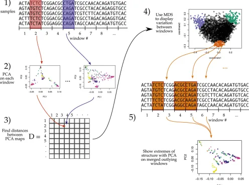
As depicted in Figure 1, the general steps to the method are: (1) divide the genome into windows, (2) summarize the pat-terns of relatedness in each window, (3) measure dissimilar-ity in relatedness between each pair of windows, (4) visualize the resulting dissimilarity matrix using multidimensional scaling (MDS), and (5) combine similar windows to more accurately visualize local effects of population structure using PCA.
PCA in genomic windows
To begin, wefirst recoded sampled genotypes as numeric
matrices in the usual manner, by recording the number of nonreference alleles seen at each locus for each sample. We then divided the genome into contiguous segments (win-dows) and applied PCA as described in McVean (2009) separately to the submatrices that corresponded to each window. The choice of window length entails a tradeoff between signal and noise, since shorter windows allow better resolution along the genome but provide less pre-cise estimates of relatedness. A method for choosing a window length to balance these considerations is given in the Appendix.
Precisely, denote by Z the L3N recoded genotype
matrix for a given window (Lis the number of SNPs and
N is the sample size), and by Zs the mean of nonmissing
entries for allele s, so thatZs¼n1s P
jZsj;where the sum is
over the ns nonmissing genotypes. We first compute the
mean-centered matrix, X, as Xsi¼Zsi2Zs; and
preserv-ing misspreserv-ingness (this mean-centerpreserv-ing makes the result in-dependent of the choice of reference allele, exactly if there is no missing data, and approximately otherwise).
Next, we find the covariance matrix of X, denoted C,
asCij¼m1 ij21
P
sXsiXsj2m 1 ijðmij21Þ
P sXsi
P
are over themijsites, where both sampleiand samplejhave
nonmissing genotypes. The principal components (PCs) are
the eigenvectors ofC, normalized to have Euclidean length
equal to 1, and ordered by magnitude of the eigenvalues.
The top two-to-five PCs are generally good summaries of
population structure; for ease of visualization we usually only
use thefirst two (referred to asPC1 andPC2), and check that
results hold using more. The above procedure can be per-formed on any subset of the data; for future reference, denote byPC1jandPC2jthe result after applying to all SNPs in thejth
window (however, note that our measure of dissimilarity be-tween windows does not depend on PC ordering).
Similarity of patterns of relatedness between windows
We think of the local effects of population structure as being
summarized by the relativeposition of the samples in the
space defined by the top PCs. However, we do not compare
patterns of relatedness of different genomic regions by
di-rectly comparing the PCs, since rotations or reflections of
these imply identical patterns of relatedness. Instead, we
compare the low-dimensional approximations of the local
covariance matrices obtained using the topk PCs, which is
invariant under reordering of the PCs, reflections, and
rota-tions, and yet contains all other information about the PCs
(for results shown here, we use k¼2:) Furthermore, to
remove the effect of artifacts such as mutation rate variation, we also rescale each approximate covariance matrix to be of similar size (precisely, so that the underlying data matrix has trace norm equal to 1).
To do this, define theN3kmatrixVðiÞso thatVðiÞℓ;theℓth
column ofVðiÞ;is equal to theℓthPC of theithwindow,
mul-tiplied by
lℓi.Pkm¼1lmi; 1=2
;wherelℓiis theℓtheigenvalue
of the genetic covariance matrix. Then, the rescaled, rankk
approximate covariance matrix for theithwindow is
MðiÞ ¼X
k
ℓ¼1
VðiÞℓVðiÞTℓ: (1)
To measure the similarity of patterns of relatedness for
theithandjthwindows, we then use Euclidean distanceD
ij
between the matrices M(i) and M(j), defined by D2 ij¼ P
kℓ
MðiÞk;ℓ2MðjÞk;ℓ2:
The goal of comparing PC plots up to rotation and reflection
turned out to be equivalent to comparing rank-k
approxima-tions to local covariance matrices. This suggests instead di-rectly comparing entire local covariance matrices. However, with thousands of samples and tens of thousands of windows, computing the distance matrix would take months of CPU
time while, as defined above,Dcan be computed in minutes
us-ing the followus-ing method. Since for square matricesAandB,
P ij
Aij2Bij 2
¼Pij
A2 ijþB2ij
22 trðATBÞ; then due to the
orthogonality of eigenvectors and the cyclic invariance of trace,
Dijcan be computed efficiently as
Dij¼ Pk
ℓ¼1l2ℓi Pk
ℓ¼1lℓi 2þ
Pk
ℓ¼1l2ℓj Pk
ℓ¼1lℓj 222
Xk
ℓ;m¼1
VðiÞTVðjÞ
2 ℓm 0 B @ 1 C A
1=2
:
(2)
Visualization of results
We use MDS to visualize relationships between windows as
summarized by the dissimilarity matrixD. MDS produces a set
ofmcoordinates for each window that give the arrangement
in m-dimensional space that best recapitulates the original
distance matrix. For results here, we usem¼2 to produce
one- or two-dimensional visualizations of relationships
be-tween windows’patterns of relatedness.
We then locate variation in patterns of relatedness along the genome by choosing collections of windows that are nearby in MDS coordinates and map their positions along the genome. A visualization of the effects of population structure across the entire collection is formed by extracting the corresponding genomic regions and performing PCA on all aggregated regions.
Testing
We tested the method using two types of simulation. First, to
verify expected behavior, we simulated“genomes”as an
in-dependent sequence of correlated Gaussian“genotypes,”
us-ing a different covariance matrix in thefirst quarter, middle
half, and last quarter of the chromosome. The details of the simulation, also designed to detect sensitivity to PC switch-ing, are given in the Appendix. To verify robustness to miss-ing data, we ran the method after randomly droppmiss-ing 50% of
the genotypes in thefirst half of the genome; if the method is
misled by missing data, then it will distinguish the two halves of the chromosome rather than the segments having different covariance matrices.
To provide a realistic test, we next used forward-time, indi-vidual-based simulations, implemented using SLiM v3 (Haller and Messer 2017), which are described in detail in the Appen-dix. To provide realistic population structure for PCA to identify, each simulation had at least 5000 diploid individuals, living across a continuous square range, with Gaussian dispersal and local density-dependent competition. Each genome was
modeled on human chromosome 7, which is 1:543108-bp
long, with an overall recombination rate of 1.6785 crossovers per chromosome per generation. To improve speed, we used
tskit (Kelleher et al.2018) to record tree sequences in SLiM
(Halleret al.2018) and to add neutral mutations afterward, at
a rate of 1029per bp per generation. Most simulations were
neutral, but we also included linked selection of two types. First, we introduced selected mutations into two regions,
which extended from one-third to one-half and from fi
ve-sixths to the end of the genome respectively. These had
selection coefficients from a Gamma distribution with shape
2 and mean 0.005 at a rate of 10210 per bp, which were
either beneficial (with probability 1/30) or deleterious
(oth-erwise). Second, to roughly model a recent expansion fol-lowed by local adaptation, we introduced mutations in the same manner as above, except that mutations were no
longer unconditionally deleterious or beneficial: each
selec-tion coefficient was multiplied by a factor depending on the
spatial location of the individual being evaluated, varying
linearly from21 at the left side of the range to +1 at the
right edge. In all simulations, genome-wide PCA displayed a map of the population range, as expected.
Data sets
We applied the method to genomic data sets with good
geo-graphic sampling: 380 AfricanDrosophila melanogasterfrom
theDrosophilaGenome Nexus (Lacket al.2015), a world-wide data set of humans, 3965 humans from several locations
worldwide from the POPRES data set (Nelson et al.2008),
and 263 Medicago truncatulafrom 24 countries around the
Mediterranean basin (a range-wide data set of the partially
selfing weedy annual plant from theM. truncatulaHapMap
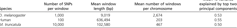
Project) (Tanget al.2014), as summarized in Table 1.
D. melanogaster: We used whole-genome sequencing data
from the DrosophilaGenome Nexus (http://www.johnpool.
net/genomes.html; Lack et al. 2015), consisting of the
Drosophila Population Genomics Project phases 1–3
(Langleyet al.2012; Poolet al.2012) and additional African
genomes (Lack et al. 2015). After removing 20 genomes
with.8% missing data, we were left with 380 samples from
16 countries across Africa and Europe. Since theDrosophila
samples are from inbred lines or haploid embryos, we treat the samples as haploid when recoding: regions with residual heterozygosity were marked as missing in the original data
set; we also removed positions with . 20% missing data.
Each chromosome arm we investigated (X, 2L, 2R, 3L, and 3R) has 2–3 million SNPs; PCA plots for each arm are shown in Supplemental Material, Figure S1.
Human:We also used genomic data from the entire POPRES
data set (Nelsonet al.2008), which has array-derived
than the other data sets, which are each derived from whole-genome sequencing. We excluded the sex somes and the mitochondria. PCA plots for each chromo-some, separately, are shown in Figure S2.
M. truncatula: Finally, we used whole-genome sequencing
data from the M. truncatula HapMap Project (Tang et al.
2014), which has 263 samples from 24 countries, primarily distributed around the Mediterranean basin. Each of the eight chromosomes has 3–5 million SNPs; PCA plots for these are shown in Figure S3. We did not use the mitochondria or chloroplasts.
Data availability
The methods described here are implemented in an
open-source R package available athttps://github.com/petrelharp/
local_pca, as well as scripts to perform all analyses from VCF
files at various parameter settings.
Data sets are available as follows: human (POPRES) at
dbGaP with accession number phs000145.v4.p2, Medicago
at theMedicagoHapMaphttp://www.medicagohapmap.org/,
andDrosophilaat theDrosophilaGenome Nexus,http://www.
johnpool.net/genomes.html. Supplemental material available
at Figshare:https://doi.org/10.25386/genetics.7324526.
Results
In all three data sets—a worldwide sample of humans, African
D. melanogaster, and a range-wide sample ofM. truncatula—
PCA plots vary along the genome in a systematic way, showing strong chromosome-scale correlations. This implies that varia-tion is due to meaningful heterogeneity in a biological process, since noise due to randomness in choice of local genealogical trees is not expected to show long-distance correlations. Below, we discuss the results and likely underlying causes.
Validation
Simple non-population-based simulations with Gaussian ge-notypes showed that the method performs as expected, clearly separating regions of the genome with different underlying covariance matrices without being affected by extreme dif-ferences in amount of missing data (Figure S4). This simula-tion also verifies insensitivity to ordering of top PCs, since it was performed using a covariance matrix with the top two eigenvalues equal, so that the order of empirical eigenvectors (PCs) switches randomly.
Individual-based simulations using SLiM (Haller and Messer 2017) allowed us to test the effects of recombination
and mutation rate variation, as well as linked selection. As expected, varying recombination rate stepwise by a factor of 64 did not induce patterns in the MDS visualizations corre-lated with recombination rate (Figure S5). Since varying
mu-tation rate with afixed recombination map is equivalent to
varying the recombination map and remapping windows, this also indicates that the method is not misled by variation in mutation rate. On the other hand, a recombination map with hotspots [the HapMap human female map for
chromo-some 7 (International Hap Map Consortiumet al.2007)]
in-duced outliers at long regions of low recombination rate (also as expected).
Simulations with linked selection produced mixed results
(Figure S6). The method strongly identified the distinct
re-gions in the simulation with spatially varying linked selection.
It also identified the regions (although less unambiguously)
with constant selection and stepwise varying recombination rate, but did not clearly identify them with constant recom-bination rate. The differences in power between these three scenarios are likely explained by varying strength of linked selection; the simulation with spatially varying selection was also the case with strongest positive selection, and recombi-nation rates were overall lower in the simulation with step-wise varying recombination rate than in the simulation with constant rate. These tests are not meant to be a comprehensive survey of linked selection, but only to demonstrate that linked selection can produce signals similar to what we see in real data.
D. melanogaster
We applied the method to windows of average length 9 kbp across chromosome arms 2L, 2R, 3L, 3R and X separately. The
first column of Figure 2 is an MDS visualization of the matrix
of dissimilarities between genomic windows: in other words, genomic windows that are closer to each other in the MDS plot show more similar patterns of relatedness. For each chro-mosome arm, the MDS visualization roughly resembles a tri-angle, sometimes with additional points. Since the relative position of each window in this plot shows the similarity be-tween windows, this suggests that there are at least three
extreme manifestations of population structure typified
by windows found in the “corners”of the figure, and that
other windows’patterns of relatedness may be a mixture of
those extremes. The next two columns of Figure 2 depict the two MDS coordinates of each window, plotted against the
window’s position along the genome, to show how the plot
of thefirst column is laid out along the genome. The patterns
did not depend on the number of PCs used (see Figure S7 for Table 1 Descriptive statistics for each data set used
Species
Number of SNPs per window
Mean window length (bp)
Mean number of windows per chromosome
Mean % variance explained by top two principal components
D. melanogaster 1,000 9,019 2,674 0.53
Human 100 636,494 203 0.55
the same plot withk¼5 PCs) and are only weakly correlated with variation in missingness (see Figure S8).
To help visualize how clustered windows with similar patterns of relatedness are along each chromosome arm, we selected three extreme windows in the MDS plot and the 5% of windows that are closest to it in the MDS
coordi-nates, then highlighted these windows’positions along the
genome, and created PCA plots for the windows, combined. Representative plots are shown for three groups of windows on each chromosome arm in Figure 2 (groups are shown in
color) and in Figure S9 (PCA plots). The latter plots are quite different, showing that genomic windows in different re-gions of the MDS plot indeed show quite different patterns of relatedness.
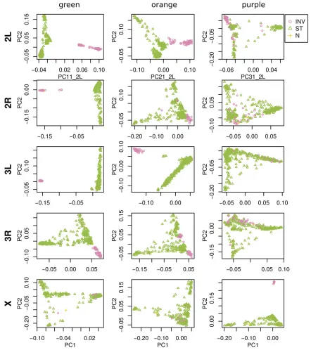
The most striking variation in patterns of relatedness turns out to be explained by several large inversions that are poly-morphic in these samples, as discussed in Corbett-Detig and
Hartl (2012) and Langleyet al.(2012). To depict this, Figure
arm 2L as an example, the two regions of similar, extreme
patterns of relatedness shown in green in the first row of
Figure 2 lie directly around the breakpoints of the inversion
In(2L)t, and the PCA plots in thefirst rows of Figure 3 show
that patterns of relatedness here are mostly determined by inversion orientation. The regions shown in purple on chro-mosome 2L lie near the centromere and have patterns of
re-latedness reflective of two axes of variation, seen in Figure 3
and Figure S9, which correspond roughly to latitude within
Africa and to degree of “cosmopolitan” admixture,
respec-tively [see Lack et al. (2015) for more about admixture in
this sample]. The regions shown in orange on chromosome 2L mostly lie inside the inversion and show patterns of re-latedness that are a mixture between the other two, as expected due to recombination within the (long) inversion
(Guerrero et al. 2011). Similar results are found in other
Figure 3 PCA plots for the three sets of genomic windows colored in Figure 2, on each chromosome arm ofD. melanogaster. In all plots, each point represents a sample. Thefirst column shows the combined PCA plot for windows whose points are colored green in Figure 2; the second is for orange windows; and the third is for purple windows. In each, samples are colored by orientation of the polymorphic inversions In(2L)t, In(2R)NS, In(3L)OK, In(3R)K, and In(1)A, respectively [data from Lacket al.(2015)]. In each,“INV”denotes an inverted genotype,“ST”denotes the standard orientation, and
chromosome arms, albeit complicated by the coexistence of more than one polymorphic inversion; however, each break-point visibly affects patterns in the MDS coordinates (see vertical lines in Figure 2).
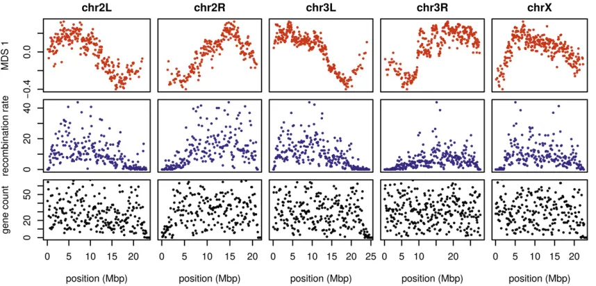
To see how patterns of relatedness vary in the absence of polymorphic inversions, we performed the same analyses after removing, for each chromosome arm, any samples car-rying inversions on that arm. In the results, shown in Figure 4 and Figure S10, the striking peaks associated with inversion breakpoints are gone, and previously smaller-scale variation now dominates the MDS visualization. For instance, the ma-jority of the variation along 3L in Figure 2 is on the left end of the arm, dominated by two large peaks around the inversion breakpoints; there is also a relatively small dip on the right end of the arm (near the centromere). In contrast, Figure 4 and Figure S10 show that after removing polymorphic inver-sions, remaining structure is dominated by the dip near the centromere. Without inversions, variation in patterns of re-latedness shown in the MDS plots follows similar patterns to
that previously seen in D. melanogasterrecombination rate
and diversity (Langleyet al.2012; Mackayet al.2012).
In-deed, correlations between the recombination rate in each
window and the position on the first MDS coordinate are
highly significant (Spearman’sr¼0:54;p,2310216;
Fig-ure 4 and FigFig-ure S11). This is consistent with the hypothesis that variation is due to selection, since the strength of linked selection increases with local gene density, measured in units of recombination distance. The number of genes—measured as the number of transcription start and end sites within each
window—was not significantly correlated with MDS
coordi-nateðp¼0:22Þ:
Human
As we did for the Drosophiladata, we applied our method
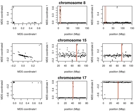
separately to all 22 human autosomes. On each, variation in patterns of relatedness was dominated by a small number of windows having similar patterns of relatedness to each other that differed dramatically from the rest of the chromosome. These may primarily be inversions: outlying windows coin-cide with three of the six large polymorphic inversions
de-scribed in Antonacci et al. (2009), notably a particularly
large, polymorphic inversion on 8p23 (Figure 5). Similar plots for all chromosomes are shown in Figure S12, Figure S13, and Figure S14. PCA plots of many outlying windows show a characteristic trimodal shape (shown for chromosome 8 in Figure S15), presumably distinguishing samples having each of the three diploid genotypes for each inversion orien-tation (although we do not have data on orienorien-tation status). This trimodal shape has been proposed as a method to iden-tify inversions (Ma and Amos 2012), but distinguishing this hypothesis from others, such as regions of low recombination rate, would require additional data.
We also applied the method on all 22 autosomes together, and found that, remarkably, the inversion on chromosome 8 is still the most striking outlying signal (Figure S16). Further
investigation with a denser set of SNPs, allowing a finer
genomic resolution, may yield other patterns.
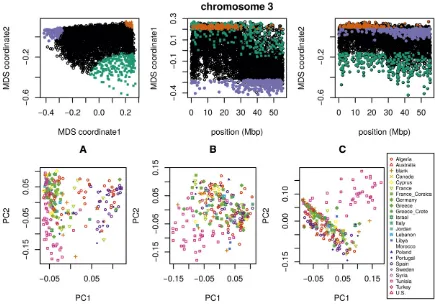
M. truncatula
Unlike the other two species, the method applied separately
on all eight chromosomes of M. truncatula showed similar
patterns of gradual change in patterns of relatedness across Figure 4 The effects of population structure without inversions is correlated to recombination rate inD. melanogaster. Thefirst plot (in red) shows the
each chromosome, with no indications of
chromosome-specific patterns. This consistency suggests that the factor
affecting the population structure for each chromosome is the same, as might be caused by varying strengths of linked se-lection. To verify that variation in the effects of population structure is shared across chromosomes, we applied the method to all chromosomes together. Results for chromo-some 3 are shown in Figure 6 and other chromochromo-somes are
similar: across chromosomes, the high values of thefirst MDS
coordinate coincide with the position of the heterochromatic regions surrounding the centromere, which often have lower gene density and may therefore be less subject to linked se-lection. To verify that this is a possible explanation, we counted the number of genes found in each window using
gene models in Mt4.0 from jcvi.org (Tanget al.2014), which
are shown juxtaposed with thefirst MDS coordinate of each
window in Figure 7 and are significantly correlated, as shown
in Figure S17 (values shown are the number of start and end positions of each predicted mRNA transcript, divided by two, assigned to the nearest window.) However, other genomic
features, such as distance to centromere, show roughly the same patterns, so we cannot rule out alternative hypotheses.
In particular,fine-scale recombination rate estimates are not
available in a form mappable to Mt4.0 coordinates [although
those in Paapeet al.(2012) appear visually similar].
The results were highly consistent across window sizes, window types (SNPs or bp), and number of PCs, as shown in Table S2.
Discussion
(Fitzpatricket al.2010; Staubachet al.2012; Huffordet al.
2013; Brandvain et al. 2014; Pool 2015), local adaptation
(Lenormand 2002; Wang and Bradburd 2014), and inversion polymorphisms (Kirkpatrick 2010; Kirkpatrick and Barrett 2015), local PCA may prove to be a useful exploratory tool to discover important genomic features.
We now discuss possible implications of this variation in the effects of population structure, the impact of various param-eter choices in implementing the method, and possible addi-tional applications.
Chromosomal inversions
A major driver of variation in patterns of relatedness in the two data sets we examined seems to be inversions. This may be
common, but the example ofM. truncatulashows that
poly-morphic inversions are not ubiquitous. PCA has been pro-posed as a method for discovering inversions (Ma and Amos 2012); however, the signal left by inversions likely cannot be distinguished from long haplotypes under balanc-ing selection or simply regions of reduced recombination without additional lines of evidence. Inversions show up in our method because across the inverted region, most gene trees share a common split that dates back to the origin of the inversion. However, in many applications, inversions are a
nuisance. For instance, SMARTPCA (Patterson et al.2006)
reduces their effect on PCA plots by regressing out the effect of linked SNPs on each other. Removing samples with the less common orientation of each inversion reduced, but did not
eliminate, the signal of inversions seen in theD. melanogaster
data set, demonstrating that the genomic effects of tran-siently polymorphic inversions may outlast the inversions themselves.
Genealogical noise?
Thefield of phylogenetics has long had to deal with the fact
that there can be a great number of different local phylogenies
along the genome, even between species (Aviseet al.1983;
Pamilo and Nei 1988; Hobolth et al. 2007). The
within-species patterns we observe might contribute to such incom-plete lineage sorting among future descendant species of a given population. The neutral distribution of variation in these patterns has been used to infer demographic history, both be-tween species (Slatkin and Pollack 2006) and within species
(Beeravolu et al. 2018). If these distinct phylogenies are
sister taxa shows clear signs of selection, as for instance in the
wild tomato clade (Peaseet al.2016).
The effect of selection
Neutral processes are not expected to produce the chromo-some-scale correlations we see in patterns of relatedness in the
M. truncatulaandD. melanogasterdata sets, because corre-lations in patterns of relatedness induced by neutral process-es should extend no further than doprocess-es linkage disequilibrium
(i.e., much less than a chromosome’s length). This suggests
that they are produced by linked selection, a hypothesis backed up by correlations with gene density and recombina-tion rate. We have also shown with simularecombina-tions that linked selection can, in at least some circumstances, produce the sorts of patterns we observe. How might selection cause var-iation in patterns of relatedness? For instance, background selection (the effect on linked sites of selection against
dele-terious mutations) (Charlesworthet al.1993, Charlesworth
2013) can informally be thought of as reducing the number of potential contributors to the gene pool in regions of the ge-nome with many possible deleterious mutations (Hudson and Kaplan 1995). For this reason, if it acts in a spatial con-text, it is expected to induce samples from nearby locations to cluster together more frequently. Therefore, regions of the genome harboring many targets of local adaptation may show similar patterns, since migrant alleles in these regions will be selected against, and so locally gene trees will more
closely reflect spatial proximity. Other forms of selection,
such as hard sweeps on new mutations, repeated selection
on standing variation, local adaptation, or temporallyfl
uctu-ating selection, could clearly lead to variation in geographic patterns of relatedness in a similar way.
of introgressed Neanderthal DNA along the genome is due to selection against Neanderthal genes, leading to greater introgression in regions of lower gene density (Harris and
Nielsen 2016; Juric et al. 2016). African D. melanogaster
are thought to have a substantial amount of recently intro-gressed genome from cosmopolitan sources; if selection reg-ularly favors genes from one origin, this could lead to substantial variation in patterns of relatedness correlated with local gene density.
There has been substantial debate over the relative impacts of different forms of selection (e.g., Charlesworthet al.1997; Charlesworth 2012; Hedrick 2013; Pease and Hahn 2013;
Burriet al.2015; Corbett-Detiget al.2015; Harris and
Niel-sen 2016; Martinet al.2016; Phunget al.2016; Stankowski
et al.2018). These have been difficult to disentangle in part because, for the most part, theory makes predictions that are
only strictly valid in randomly mating (i.e., unstructured)
populations, and it is unclear to what extent the spatial struc-ture observed in most real populations will affect these pre-dictions. Developing a method to distinguish these forms of selection from each other and from the effects of demography
is a major challenge to thefield. It may be possible to make
progress using statistics that make stronger use of spatial in-formation, such as the variation in relatedness that we
ob-serve here, similar to the method of Beeravoluet al.(2018).
Parameter choices
There are several choices in the method that may in principle affect the results. As with whole-genome PCA, the choice of samples is important, as variation not strongly represented in the sample will not be discovered. The effects of strongly imbalanced sampling schemes are often corrected by drop-ping samples in overrepresented groups; but downweighting may be a better option that does not discard data. Next, the choice of window size may be important, although in our applications, results were not sensitive to this. Finally, which collections of genomic regions are compared to each other (steps 3 and 4 in Figure 1), along with the method used to discover common structure, will affect results. We used MDS, applied to either each chromosome separately or to the entire genome; for instance, human inversions are clearly visible as outliers when compared to the rest of their chromosomes, but genome-wide, their signal is obscured by the numerous other signals of comparable strength.
Besides window length, there is also the question of how to choose windows. In these applications, we have used non-overlapping windows with equal numbers of polymorphic sites. However, we found little change in results when using different window sizes or when measuring windows in phys-ical distance (in base pairs).
Finally, our software allows different choices for how many PCs to use in approximating the structure of each
win-dow (kin Equation 1) and how many MDS coordinates to use
when describing the distance matrix between windows, but in our exploration, changing these has not produced dramat-ically different results. However, this choice could in some
situations be important: for instance, if thekthandðkþ1Þst
PCs are sufficiently different but have similar eigenvalues,
then small amounts of noise could cause these to switch, leading to spuriously inferred differences between windows
in which one or the other was included in the topkPCs. This
does not seem to be a problem in our applications, as chang-ing the number of PCs did not affect the qualitative results. These choices are all part of more general techniques in di-mension reduction and high-didi-mensional data visualization; we encourage the user to experiment.
Applications
So-called cryptic relatedness between samples has been one of the major sources of confounding in GWAS, and so methods must account for it by modeling population structure or
kin-ship (Astle and Balding 2009; Yang et al. 2014). Modern
“mixed model”methods (e.g., Lohet al.2015) account for
this with either a single, genome-wide kinship matrix or one constructed using only sites unlinked to the focal SNP. Since the effects of population structure are not constant along the
genome, this could in principle lead to an inflation of false
positives in parts of the genome with stronger population structure than the genome-wide average. A method such as ours might be used to estimate local kinship matrices, thus providing a more sensitive correction, although doing so without removing the signal itself could be challenging. For-tunately, in our human data set this does not seem likely to have a strong effect: most variation is due to small, indepen-dent regions, possibly primarily inversions, and so may not have a major effect on GWAS. In the other species we
exam-ined, particularlyD. melanogaster, treating population
struc-ture as a single quantity would entail a substantial loss of power and could potentially be misleading.
Acknowledgments
We thank John Pool, Russ Corbett-Detig, Matilde Cordeiro, and Peter Chang for assistance with obtaining data and
interpreting results (especially the inversion status ofD.
mel-anogastersamples); Jaime Ashander and Jerome Kelleher for providing assistance in performing the simulations; and Yaniv Brandvain, Barbara Engelhardt, Charles Langley, Graham Coop, and Jeremy Berg for helpful comments and for en-couraging the project. Work on this project was supported by NSF grant number 1262645 (DBI) to PR. The authors declare no conflicts of interest.
Literature Cited
Antonacci, F., J. M. Kidd, T. Marques-Bonet, M. Ventura, P. Siswara et al., 2009 Characterization of six human disease-associated inversion polymorphisms. Hum. Mol. Genet. 18: 2555–2566.
https://doi.org/10.1093/hmg/ddp187
Astle, W., and D. J. Balding, 2009 Population structure and cryp-tic relatedness in genecryp-tic association studies. Stat. Sci. 24: 451–
Avise, J. C., J. F. Shapira, S. W. Daniel, C. F. Aquadro, and R. A. Lansman, 1983 Mitochondrial DNA differentiation during the speciation process in Peromyscus. Mol. Biol. Evol. 1: 38–56. Barton, N. H., 2000 Genetic hitchhiking. Philos. Trans. R. Soc.
Lond. B Biol. Sci. 355: 1553–1562. https://doi.org/10.1098/ rstb.2000.0716
Beeravolu, C. R., M. J. Hickerson, L. A. F. Frantz, and K. Lohse, 2018 Able: blockwise site frequency spectra for inferring com-plex population histories and recombination. Genome Biol. 19:
145.https://doi.org/10.1186/s13059-018-1517-y
Blair, A. P., 1943 Population structure in toads. Am. Nat. 77: 563–
568.https://doi.org/10.1086/281161
Brandvain, Y., A. M. Kenney, L. Flagel, G. Coop, and A. L. Sweigart, 2014 Speciation and introgression betweenMimulus nasutus andMimulus guttatus. PLoS Genet. 10: e1004410.https://doi. org/10.1371/journal.pgen.1004410
Brisbin, A., K. Bryc, J. Byrnes, F. Zakharia, L. Omberg et al., 2012 PCAdmix: principal components-based assignment of ancestry along each chromosome in individuals with admixed ancestry from two or more populations. Hum. Biol. 84: 343–
364.https://doi.org/10.3378/027.084.0401
Bryc, K., A. Auton, M. R. Nelson, J. R. Oksenberg, S. L. Hauseret al., 2010 Genome-wide patterns of population structure and admix-ture in West Africans and African Americans. Proc. Natl. Acad. Sci. USA 107: 786–791.https://doi.org/10.1073/pnas.0909559107
Burri, R., A. Nater, T. Kawakami, C. F. Mugal, P. I. Olason et al., 2015 Linked selection and recombination rate variation drive the evolution of the genomic landscape of differentiation across the speciation continuum of Ficedulaflycatchers. Genome Res. 25: 1656–1665.https://doi.org/10.1101/gr.196485.115
Busing, F. M., E. Meijer, and R. Van Der Leeden, 1999 Delete-m jackknife for unequal m. Stat. Comput. 9: 3–8.https://doi.org/ 10.1023/A:1008800423698
Charlesworth, B., 2012 The effects of deleterious mutations on evolution at linked sites. Genetics 190: 5–22.https://doi.org/ 10.1534/genetics.111.134288
Charlesworth, B., 2013 Background selection 20 years on: the Wilhelmine E. Key 2012 invitational lecture. J. Hered. 104:
161–171.https://doi.org/10.1093/jhered/ess136
Charlesworth, B., M. T. Morgan, and D. Charlesworth, 1993 The effect of deleterious mutations on neutral molecular variation. Genetics 134: 1289–1303.
Charlesworth, B., M. Nordborg, and D. Charlesworth, 1997 The effects of local selection, balanced polymorphism and back-ground selection on equilibrium patterns of genetic diversity in subdivided populations. Genet. Res. 70: 155–174. https:// doi.org/10.1017/S0016672397002954
Charlesworth, B., D. Charlesworth, and N. H. Barton, 2003 The effects of genetic and geographic structure on neutral variation. Annu. Rev. Ecol. Evol. Syst. 34: 99–125. https://doi.org/ 10.1146/annurev.ecolsys.34.011802.132359
Comeron, J. M., R. Ratnappan, and S. Bailin, 2012 The many landscapes of recombination inDrosophila melanogaster. PLoS Genet. 8: e1002905.
Corbett-Detig, R. B., and D. L. Hartl, 2012 Population genomics of inversion polymorphisms inDrosophila melanogaster. PLoS Genet. 8: e1003056 (erratum: PLoS Genet. 9).https://doi.org/ 10.1371/journal.pgen.1003056
Corbett-Detig, R. B., D. L. Hartl, and T. B. Sackton, 2015 Natural selection constrains neutral diversity across a wide range of species. PLoS Biol. 13: e1002112. https://doi.org/10.1371/ journal.pbio.1002112
Cruickshank, T. E., and M. W. Hahn, 2014 Reanalysis suggests that genomic islands of speciation are due to reduced diversity, not reduced geneflow. Mol. Ecol. 23: 3133–3157.https://doi. org/10.1111/mec.12796
Duforet-Frebourg, N., K. Luu, G. Laval, E. Bazin, and M. G. Blum, 2016 Detecting genomic signatures of natural selection with principal component analysis: application to the 1000 genomes data. Mol. Biol. Evol. 33: 1082–1093.
Efron, B., 1982 The Jackknife,the Bootstrap and Other Resampling Plans. Society for Industrial and Applied Mathematics, Philadel-phia.https://doi.org/10.1137/1.9781611970319
Ellegren, H., L. Smeds, R. Burri, P. I. Olason, N. Backströmet al., 2012 The genomic landscape of species divergence in Ficedula
flycatchers. Nature 491: 756–760. https://doi.org/10.1038/ nature11584
Fiston-Lavier, A.-S., N. D. Singh, M. Lipatov, and D. A. Petrov, 2010 Drosophila melanogaster recombination rate calcula-tor. Gene 463: 18–20.https://doi.org/10.1016/j.gene.2010. 04.015
Fitzpatrick, B. M., J. R. Johnson, D. K. Kump, J. J. Smith, S. R. Voss et al., 2010 Rapid spread of invasive genes into a threatened native species. Proc. Natl. Acad. Sci. USA 107: 3606–3610.
https://doi.org/10.1073/pnas.0911802107
Guerrero, R. F., F. Rousset, and M. Kirkpatrick, 2011 Coalescent patterns for chromosomal inversions in divergent populations. Philos. Trans. R. Soc. Lond. B Biol. Sci. 367: 430–438.https:// doi.org/10.1098/rstb.2011.0246
Haller, B. C., and P. W. Messer, 2017 SLiM 2:flexible, interactive forward genetic simulations. Mol. Biol. Evol. 34: 230–240.
https://doi.org/10.1093/molbev/msw211
Haller, B. C., J. Galloway, J. Kelleher, P. W. Messer, and P. L. Ralph, 2018 Tree-sequence recording in SLiM opens new horizons for forward-time simulation of whole genomes. bioRxiv. Available
at:https://doi.org/10.1101/407783.
Harris, K., and R. Nielsen, 2016 The genetic cost of Neanderthal introgression. Genetics 203: 881–891.https://doi.org/10.1534/ genetics.116.186890
Hedrick, P. W., 2013 Adaptive introgression in animals: examples and comparison to new mutation and standing variation as sources of adaptive variation. Mol. Ecol. 22: 4606–4618.
https://doi.org/10.1111/mec.12415
Hobolth, A., O. F. Christensen, T. Mailund, and M. H. Schierup, 2007 Genomic relationships and speciation times of human, chimpanzee, and gorilla inferred from a coalescent hidden Markov model. PLoS Genet. 3: e7. https://doi.org/10.1371/ journal.pgen.0030007
Hudson, R. R., and N. L. Kaplan, 1995 Deleterious background selection with recombination. Genetics 141: 1605–1617. Huerta-Sánchez, E., M. DeGiorgio, L. Pagani, A. Tarekegn, R. Ekong
et al., 2013 Genetic signatures reveal high-altitude adaptation in a set of Ethiopian populations. Mol. Biol. Evol. 30: 1877– 1888.https://doi.org/10.1093/molbev/mst089
Hufford, M. B., P. Lubinksy, T. Pyhäjärvi, M. T. Devengenzo, N. C. Ellstrandet al., 2013 The genomic signature of crop-wild in-trogression in maize. PLoS Genet. 9: e1003477.https://doi.org/ 10.1371/journal.pgen.1003477
International HapMap Consortium, K. A. Frazer, D. G. Ballinger, D. R. Cox, D. A. Hindset al., 2007 A second generation human haplotype map of over 3.1 million SNPs. Nature 449: 851–861.
https://doi.org/10.1038/nature06258
Juric, I., S. Aeschbacher, and G. Coop, 2016 The strength of se-lection against Neanderthal introgression. PLoS Genet. 12: e1006340.https://doi.org/10.1371/journal.pgen.100634
Kambhatla, N., and T. K. Leen, 1997 Dimension reduction by local principal component analysis. Neural Comput. 9: 1493–1516.
https://doi.org/10.1162/neco.1997.9.7.1493
Kim, Y., and W. Stephan, 2002 Detecting a local signature of ge-netic hitchhiking along a recombining chromosome. Gege-netics 160: 765–777.
Kirkpatrick, M., 2010 How and why chromosome inversions evolve. PLoS Biol. 8: e1000501. https://doi.org/10.1371/jour-nal.pbio.1000501
Kirkpatrick, M., and B. Barrett, 2015 Chromosome inversions, adaptive cassettes and the evolution of species’ ranges. Mol. Ecol. 24: 2046–2055.https://doi.org/10.1111/mec.13074
Lack, J. B., C. M. Cardeno, M. W. Crepeau, W. Taylor, R. B. Corbett-Detiget al., 2015 The Drosophila genome nexus: a population genomic resource of 623Drosophila melanogastergenomes, in-cluding 197 from a single ancestral range population. Genetics 199: 1229–1241.https://doi.org/10.1534/genetics.115.174664
Langley, C. H., K. Stevens, C. Cardeno, Y. C. Lee, D. R. Schrider et al., 2012 Genomic variation in natural populations of Drosophila melanogaster. Genetics 192: 533–598. https://doi. org/10.1534/genetics.112.142018
Lenormand, T., 2002 Geneflow and the limits to natural selec-tion. Trends Ecol. Evol. 17: 183–189.https://doi.org/10.1016/ S0169-5347(02)02497-7
Loh, P. R., G. Tucker, B. K. Bulik-Sullivan, B. J. Vilhjálmsson, H. K. Finucaneet al., 2015 Efficient Bayesian mixed-model analysis increases association power in large cohorts. Nat. Genet. 47:
284–290.https://doi.org/10.1038/ng.3190
Ma, J., and C. I. Amos, 2012 Investigation of inversion polymorphisms in the human genome using principal components analysis. PLoS One 7: e40224.https://doi.org/10.1371/journal.pone.0040224
Mackay, T. F. C., S. Richards, E. A. Stone, A. Barbadilla, J. F. Ayroles et al., 2012 TheDrosophila melanogastergenetic reference panel. Nature 482: 173–178.https://doi.org/10.1038/nature10811
Manjón, J. V., P. Coupé, L. Concha, A. Buades, D. L. Collinset al., 2013 Diffusion weighted image denoising using overcomplete local PCA. PLoS One 8: e73021. https://doi.org/10.1371/jour-nal.pone.0073021
Martin, S. H., M. Möst, W. J. Palmer, C. Salazar, W. O. McMillan et al., 2016 Natural selection and genetic diversity in the but-terfly Heliconius melpomene. Genetics 203: 525–541.https:// doi.org/10.1534/genetics.115.183285
McVean, G., 2009 A genealogical interpretation of principal com-ponents analysis. PLoS Genet. 5: e1000686. https://doi.org/ 10.1371/journal.pgen.1000686
Menozzi, P., A. Piazza, and L. Cavalli-Sforza, 1978 Synthetic maps of human gene frequencies in Europeans. Science 201: 786–
792.https://doi.org/10.1126/science.356262
Nadeau, N. J., A. Whibley, R. T. Jones, J. W. Davey, K. K. Dasma-hapatraet al., 2012 Genomic islands of divergence in hybrid-izing Heliconius butterflies identified by large-scale targeted sequencing. Philos. Trans. R. Soc. Lond. B Biol. Sci. 367: 343–
353.https://doi.org/10.1098/rstb.2011.0198
Nelson, M. R., K. Bryc, K. S. King, A. Indap, A. R. Boyko et al., 2008 The population reference sample, POPRES: a resource for population, disease, and pharmacological genetics research. Am. J. Hum. Genet. 83: 347–358. https://doi.org/10.1016/j. ajhg.2008.08.005
Novembre, J., and M. Stephens, 2008 Interpreting principal com-ponent analyses of spatial population genetic variation. Nat. Genet. 40: 646–649.https://doi.org/10.1038/ng.139
Novembre, J., T. Johnson, K. Bryc, Z. Kutalik, A. R. Boyko et al., 2008 Genes mirror geography within Europe. Nature 456: 98– 101 (erratum: Nature 456: 274). https://doi.org/10.1038/na-ture07331
Paape, T., P. Zhou, A. Branca, R. Briskine, N. Young et al., 2012 Fine-scale population recombination rates, hotspots, and correlates of recombination in theMedicago truncatula ge-nome. Genome Biol. Evol. 4: 726–737. https://doi.org/ 10.1093/gbe/evs046
Pamilo, P., and M. Nei, 1988 Relationships between gene trees and species trees. Mol. Biol. Evol. 5: 568–583.
Patterson, N., A. L. Price, and D. Reich, 2006 Population structure and eigenanalysis. PLoS Genet. 2: e190. https://doi.org/ 10.1371/journal.pgen.0020190
Pease, J. B., and M. W. Hahn, 2013 More accurate phylogenies inferred from low-recombination regions in the presence of in-complete lineage sorting. Evolution 67: 2376–2384.https://doi. org/10.1111/evo.12118
Pease, J. B., D. C. Haak, M. W. Hahn, and L. C. Moyle, 2016 Phylogenomics reveals three sources of adaptive varia-tion during a rapid radiavaria-tion. PLoS Biol. 14: e1002379.https:// doi.org/10.1371/journal.pbio.1002379
Phung, T. N., C. D. Huber, and K. E. Lohmueller, 2016 Determining the effect of natural selection on linked neutral divergence across species. PLoS Genet. 12: e1006199. https://doi.org/10.1371/ journal.pgen.1006199
Pool, J. E., 2015 The mosaic ancestry of the Drosophila genetic reference panel and theD. melanogasterreference genome re-veals a network of epistaticfitness interactions. Mol. Biol. Evol. 32: 3236–3251.
Pool, J. E., R. B. Corbett-Detig, R. P. Sugino, K. A. Stevens, C. M. Cardenoet al., 2012 Population genomics of sub-Saharan Dro-sophila melanogaster: African diversity and non-African admix-ture. PLoS Genet. 8: e1003080. https://doi.org/10.1371/ journal.pgen.1003080
Price, A. L., N. J. Patterson, R. M. Plenge, M. E. Weinblatt, N. A. Shadicket al., 2006 Principal components analysis corrects for stratification in genome-wide association studies. Nat. Genet. 38: 904–909.https://doi.org/10.1038/ng1847
Roweis, S. T., and L. K. Saul, 2000 Nonlinear dimensionality re-duction by locally linear embedding. Science 290: 2323–2326.
https://doi.org/10.1126/science.290.5500.2323
Slatkin, M., and J. L. Pollack, 2006 The concordance of gene trees and species trees at two linked loci. Genetics 172: 1979–1984.
https://doi.org/10.1534/genetics.105.049593
Stankowski, S., M. A. Chase, A. M. Fuiten, P. L. Ralph, and M. A. Streisfeld, 2018 The tempo of linked selection: rapid emergence of a heterogeneous genomic landscape during a radiation of mon-keyflowers. bioRxiv. Available at:https://doi.org/10.1101/342352. Staubach, F., A. Lorenc, P. W. Messer, K. Tang, D. A. Petrovet al., 2012 Genome patterns of selection and introgression of hap-lotypes in natural populations of the house mouse (Mus muscu-lus). PLoS Genet. 8: e1002891. https://doi.org/10.1371/ journal.pgen.1002891
Tang, H., V. Krishnakumar, S. Bidwell, B. Rosen, A. Chan et al., 2014 An improved genome release (version mt4.0) for the model legume Medicago truncatula. BMC Genomics 15: 312.
https://doi.org/10.1186/1471-2164-15-312
Turner, T. L., M. W. Hahn, and S. V. Nuzhdin, 2005 Genomic islands of speciation in Anopheles gambiae. PLoS Biol. 3: e285. Vernot, B., and J. M. Akey, 2014 Resurrecting surviving Neander-tal lineages from modern human genomes. Science 343: 1017– 1021.https://doi.org/10.1126/science.1245938
Wang, I. J., and G. S. Bradburd, 2014 Isolation by environment. Mol. Ecol. 23: 5649–5662.https://doi.org/10.1111/mec.12938
Weingessel, A., and K. Hornik, 2000 Local PCA algorithms. Neural networks. IEEE Transactions on 11: 1242–1250.
Wright, S., 1949 The genetical structure of populations. Ann. Eugen. 15: 323–354. https://doi.org/10.1111/j.1469-1809. 1949.tb02451.x
Yang, J., N. A. Zaitlen, M. E. Goddard, P. M. Visscher, and A. L. Price, 2014 Advantages and pitfalls in the application of mixed-model association methods. Nat. Genet. 46: 100–106.
https://doi.org/10.1038/ng.2876
Appendix
Choosing window length
The choice of window length entails a balance between signal and noise. In very short windows, genealogies of the samples will only be represented by a few trees, so variation between windows represents demographic noise rather than meaningful variation in patterns of relatedness. Longer windows generally have more distinct trees (and SNPs), allowing for less noisy estimation of local patterns of relatedness. However, to better resolve meaningful signal, i.e., differences in patterns of relatedness along the genome, we would like reasonably short windows.
Since we summarize patterns of relatedness using relative positions in the principal component maps, we quantify“noise”as
the standard error of a sample’s position on PC1 in a particular window, averaged across windows and samples, and“signal”as
the standard deviation of the sample’s position on PC1 over all windows, averaged over samples. The definition of eigenvectors
does not specify their sign, and so when comparing between windows we choose signs to best match each other: after choosing
PC11, for instance, if u is thefirst eigenvector obtained from the covariance matrix for window j, then we next choose
PC1j5 6u, where the sign is chosen according to which ofkPC112ukorkPC111ukis smaller.
After doing this, the mean variance across windows is
s2 signal5
1
N
X
j51
N
1
L
X
i51
L
ðPC1ij2PC1jÞ2;
wherePC1ijis the position of theithindividual onPC1 in windowj, andPC1j5ð1=NÞ PN
j51PC1ij. We estimate the standard
error for eachPC1ijusing the block jackknife (Efron, 1982; Businget al.1999): we divide thejthwindow into 10 equal-sized
pieces, and letPC1ij;kdenote thefirst principal component of this region found after removing thekthpiece; then the estimate
of the squared standard error iss2ij5 9 10
P10 k51
PC1ij;k2101 P10
ℓ51PC1ij;ℓ 2
. Averaging over samples and windows,
s2 noise5
1
N
X
j51
N
1
L
X
i51
L
s2
ij:
For the main analysis, we defined windows to each consist of the same number of neighboring SNPs, and calculateds2
signaland s2
noisefor a range of window sizes (i.e., numbers of SNPs). For our main results we chose the smallest window for whichs2signal
was consistently larger thans2
noise(but checked other sizes); the values for various window sizes acrossDrosophila chromo-somes are shown in Table S1. In the cases we examined, we found nearly identical results after varying window size, and choosing windows to be of the same physical length (in bp) rather than in numbers of SNPs.
Simulations
We implemented two types of simulation:first, simple simulations of Gaussian“genotypes”where the expectation of variation in
“population structure”was clear; and next, individual-based simulations with explicit genomes, using SLiM.
Gaussian simulations
We simulated genotypes at each locus independently, drawing each vector of genotypes from a multivariate Gaussian
distribution with zero mean and covariance matrixS. Sampled individuals came from three populations, and eachSijdepends
on which populations the individualsiandjare in, as well as the location along the chromosome. There are three
population-level mean relatedness matrices along the genome, which apply to thefirst quarter (Sð1Þ), the middle half (Sð2Þ), and the last
quarter (Sð3Þ), respectively:
Sð1Þ5
2
400::7525 00::2575 00::00 0:0 0:0 1:0
3 5
Sð2Þ5
2
410::00 00::750 00:25:0 0:0 0:25 0:75
3 5
Sð3Þ5
2
400:75:0 01::00 00:25:0
0:25 0:0 0:75
If indiviudals i and j are in populations pðiÞ and pðjÞ respectively, then the covariance between their genotypes is
Sij5SpðiÞ;pðjÞ, using the appropriate S for that segment of the genome. The variance of individual i’s genotype is
Sii5SpðiÞ;pðiÞ10:1.
Wefirst created“genotypes”in this way withfifty individuals from each of the three populations; running our method on a
genome with 99 windows of 400 loci each produced thefirst plot in Supplementary Figure S4. These matrices are chosen so
that the top two eigenvaluesSare the same (both 50.1), and so the ordering of the top two PCs is arbitrary. If our method was
sensitive to PC ordering, then half the windows in each region that have one ordering would cluster with each other, separate from the other half.
We then marked each genotype in thefirst half of the chromosome as missing, independently, with probability 1=2 and ran
our method again, producing the second plot of Supplementary Figure S4. If our method was influenced by missing data, we
would expect thefirst half of the chromosome to separate from the second in the MDS plot.
SLiM simulations
Our SLiM simulations were constructed as follows. Individuals are diploid, and genomes have a length of 153,520,244 bp.
Recombination was either (a) flat, with a constant rate of 1029; (b) according to the human female HapMap map for
chromosome 7; or (c) constant in each of seven equal-sized regions, beginning at 2:0431028, descending by a factor of four
for three steps, and then ascending by a factor of four for three steps, so that the middle seventh has the lowest recombination
rate, and the outer two sevenths has a rate 64 times higher. Selected mutations are introduced at a rate of 10210per bp per
individual per generation, and have selection coefficients drawn from a Gamma distribution with mean 0.005 and shape 2;
each coefficient are either positive or negative with probabilities 1=30 and 29=30 respectively. Each simulation was run for
50,000 generations.
Each individual has a spatial position in the two-dimensional square of widthW58. Each time step, each individual chooses
the nearest other to mate with, producing a random, Poisson distributed number of offspring with mean 1=3. Offspring are
assigned random spatial locations displaced from their parent’s by a bivariate Gaussian with mean zero and standard deviation
s50:2, reflected to stay within the habitat range.
Each individual survives to the next time step with probability equal to their fitness. Fitness values are determined
multiplicatively by the effects of each mutation, but are multiplied by an additional factor determined by the local density of individuals. This factor is equal tor=ð11CÞ, wherer52pKs2is the carrying capacity per circle of radiuss;K5100 is the
mean equilibrium population density; andCis the sum of a Gaussian kernel with standard deviations50:1 between the focal
individual and all other individuals within distance 3s. To avoid edge effects,fitnesses are further multiplied by minð1;zÞ,
where z is the distance to the nearest boundary. This produces populations that fluctuate at equilibrium around 6,000
individuals in total, fairly evenly spread across the square.
In one additional simulation, we modifiedfitnesses by multiplying the selective effect of each allele in each individual by