ABSTRACT
BUCH, NILS. Inventory Models Without Explicit Fixed Ordering Costs. (Under the direction of Russell King and Donald Warsing.)
Our research investigates new methods for solving single and multiple period,
finite-horizon, inventory problems when the number of orders allowed during the horizon is limited.
Existing literature has solved the question of how many goods to order when there is only one
order available to make at the beginning of the horizon, as well as how many goods to order
when there is an explicit and known fixed ordering cost incurred upon the placing of an order.
Our models extend the problem to the case when the fixed ordering costs are either unknown
or very difficult to estimate.
The classical "newsvendor problem" in the management sciences solves for the optimal
ordering quantity when there is a single period with a known single demand distribution. Our
first research question is how to extend this classical model when there exist two opportunities
for ordering within the horizon. We develop analytical formulations to solve this extension
optimally.
An extension of the single-period case with one replenishment is a general multiple-period
model with multiple (restricted) replenishment opportunities, without an explicitly stated
fixed ordering cost. To solve this problem, we employ a Markov Decision Process-based
solution methodology, where the costs of over-ordering and under-ordering are weighed
against each other to determine the optimal ordering quantity for any period, when the
decision maker has a given number of orders remaining. We also investigate an approximation
to solve this problem near-optimally. We extend this model to account for price markdown
opportunities.
Our research also solves a related problem when the demand distribution parameters
are unknown. We evaluate the extent to which additional orders can alleviate some of the
simulation and Markov Decision Process solution methodology that utilizes both optimal and
near-optimal solutions for the known demand case in a simulation environment consisting
of unknown seasonal demand. We show the profit difference in the known and unknown
Inventory Models Without Explicit Fixed Ordering Costs
by Nils Buch
A dissertation submitted to the Graduate Faculty of North Carolina State University
in partial fulfillment of the requirements for the Degree of
Doctor of Philosophy
Industrial Engineering
Raleigh, North Carolina
2013
APPROVED BY:
Russell King
Co-chair of Advisory Committee
Anita Vila-Parrish
Thom Hodgson Donald Warsing
BIOGRAPHY
Nils Buch hails from Braunschweig, Germany. He and his family moved to the United States
in 1990, settling in South Carolina. He received his B.S. (2007) and Masters (2009) degrees in
TABLE OF CONTENTS
LIST OF TABLES . . . v
LIST OF FIGURES. . . vi
Chapter 1 Introduction . . . 1
1.1 Description of the general problem . . . 1
1.1.1 Season length . . . 2
1.1.2 Demand and forecast reestimation . . . 2
1.1.3 Basic costs . . . 4
1.1.4 Lead time . . . 6
1.1.5 Revenue and markdowns . . . 6
1.1.6 Lost sales . . . 7
1.1.7 Multiple products . . . 7
1.2 Description of models considered . . . 8
1.3 General model formulation . . . 9
Chapter 2 A Single Period Inventory Model with Known Demand Distribution Pa-rameters . . . 12
2.1 Introduction . . . 12
2.2 Literature Review . . . 14
2.3 No Compensation Model . . . 20
2.3.1 Results for uniformly distributed demand . . . 25
2.3.2 Results for Exponentially distributed demand . . . 38
2.3.3 Results for Normally distributed demand . . . 38
2.3.4 Results for Negative Binomial demand distribution . . . 39
2.4 Compensation Model . . . 42
2.4.1 Option compensation arrangement . . . 44
2.4.2 Fixed cost compensation arrangement . . . 47
2.4.3 Downpayment compensation arrangement . . . 49
2.4.4 Higher unit cost compensation arrangement . . . 50
2.4.5 Comparing methods . . . 53
2.5 Other Embellishments . . . 55
2.5.1 Uniform distribution . . . 56
2.5.2 Holding cost model . . . 58
2.6 Conclusion . . . 65
Chapter 3 A Multiple Period Inventory Model with Known Demand Distribution Pa-rameters . . . 66
3.1 Introduction . . . 66
3.2 Definitions and Notation . . . 67
3.4 Numerical Experiments . . . 72
3.4.1 Demand seasonality . . . 72
3.4.2 Experimental design . . . 74
3.5 Heuristic Solution . . . 82
3.6 Summary . . . 88
Chapter 4 A Multiple Period Inventory Model with Restricted Replenishment and Unknown Demand Distribution Parameters . . . 89
4.1 Introduction . . . 89
4.2 Literature Review . . . 91
4.3 Model Formulation and Demand Reestimation . . . 94
4.4 Results for a Specified Forecast Error . . . 102
4.5 Results for a Stochastic Forecast Error . . . 104
4.5.1 Coverage policies . . . 109
4.6 Summary and Conclusion . . . 114
Chapter 5 A Multiple Period Inventory Problem with Restricted Replenishment and Price Markdown Opportunities . . . 121
5.1 Introduction . . . 121
5.2 A Multi-Period, Finite-Horizon Inventory Model with Markdown . . . 123
5.2.1 Formulation . . . 123
5.2.2 Modeling demand . . . 125
5.3 Analytical Results . . . 126
5.3.1 Deterministic demand . . . 128
5.3.2 Stochastic demand . . . 132
5.4 Value of a Markdown Opportunity . . . 136
5.5 Conclusion . . . 146
Chapter 6 Conclusion . . . 149
References . . . 151
Appendix . . . 153
Appendix A Appendix . . . 154
A.1 Chapter 2 appendix . . . 154
LIST OF TABLES
Table 2.1 Experimental set . . . 26 Table 2.2 Analysis of variance results . . . 28
Table 3.1 Experimental parameters . . . 74
Table 3.2 Range of parameters from which 250 random instances were selected for
numerical results . . . 82 Table 3.3 Results for the ˆst,S∗
t|sˆt
policy for 250 random instances . . . 84
Table 3.4 Results of ˆSt, ˆst
policy, profit loss from optimal for 250 random instances 85
Table 4.1 Range of parameters from which 250 random instances were selected for
numerical results . . . 102
Table 4.2 Front-heavy seasonality, value of replenishments and information summary117
Table 4.3 Centered seasonality, value of replenishments and information summary 118
Table 4.4 Back-heavy seasonality, value of replenishments and information summary119
Table 5.1 Experimental design parameters range,δ=0.5,e(δ) =2 . . . 138
Table A.1 Comparison of newsvendor solution results to single period replenish-ment solution . . . 164 Table A.2 Profit and value of replenishment opportunity results for 81 parameter
instances . . . 166 Table A.3 Profit and value of replenishment opportunity results for 81 parameter
LIST OF FIGURES
Figure 2.1 No replenishment . . . 22 Figure 2.2 Replenishment with salvage . . . 22 Figure 2.3 Replenishment and lost sales . . . 23
Figure 2.4 Histogram of profit gain with single replenishment, 27 instances,
Uni-form distribution . . . 26
Figure 2.5 Comparing expected total units ordered over, 27 instances, Uniform
distribution . . . 27
Figure 2.6 ANOVA results for % profit increase with replenishment, salvage value
term . . . 29
Figure 2.7 ANOVA results for % profit increase with replenishment, lost sales penalty
term . . . 30
Figure 2.8 ANOVA results for % profit increase with replenishment, revenue term . 31
Figure 2.9 ANOVA results for % sales increase with replenishment, revenue term . 32
Figure 2.10 ANOVA results for % sales increase with replenishment, lost sales penalty term . . . 33 Figure 2.11 ANOVA results for % sales increase with replenishment, salvage value term 34 Figure 2.12 ANOVA results for % lost sales decrease with replenishment, revenue term 35 Figure 2.13 ANOVA results for % lost sales decrease with replenishment, lost sales
penalty term . . . 36 Figure 2.14 ANOVA results for % lost sales decrease with replenishment, salvage
value term . . . 37
Figure 2.15 Optimal order quantities with lows,D ∼N (30,σ),c =1,r =2,p=.3 . . 39
Figure 2.16 Optimal order quantities with highs,D ∼N (30,σ),c =1,r =2,p=.3 . 40
Figure 2.17 Three Negative binomial distributions considered, mean=55 . . . 40
Figure 2.18 Expected total ordering quantity . . . 41 Figure 2.19 Supply chain benefit of replenishment opportunity (no premium),
nega-tive binomial demand distribution with medium variance . . . 42
Figure 2.20 Retailer’s and supplier’s profit change (in %), representing their maxi-mum and minimaxi-mum option price requirements, 27 instances with Uni-form demand distribution . . . 46 Figure 2.21 Retailer’s maximum and supplier’s minimum option price to enter into
replenishment contract, 27 instances with Negative binomial distribu-tion and medium variance . . . 46 Figure 2.22 Negotiation range for fixed replenishment cost from retailer to supplier,
Uniform distribution . . . 48 Figure 2.23 Negotiation range for fixed replenishment cost from retailer to supplier,
27 instances with Negative binomial distribution and medium variance 49
Figure 2.24 Negotiation range for down payment method, 27 instances with Negative
Figure 2.25 Negotiation range for higher replenishment unit cost method, 27
in-stances with Negative binomial distribution and medium variance . . . . 53
Figure 2.26 Retailer profit equivalency between fixed cost and higher unit cost com-pensation arrangement comparison, Uniform distribution . . . 54
Figure 2.27 Retailer profit equivalency between fixed cost and down payment com-pensation arrangements, Uniform distribution . . . 55
Figure 2.28 Method 2: Convergence to optimal solution using iteration method . . . 63
Figure 2.29 Numerical example ofQ∗ 2 andQ1∗as functions of each other . . . 64
Figure 2.30 Sensitivity of optimal solution to holding cost,h . . . 64
Figure 3.1 Timeline of events within a period . . . 68
Figure 3.2 Ordering is best . . . 71
Figure 3.3 Not Ordering is best . . . 71
Figure 3.4 Front-heavy demand . . . 72
Figure 3.5 Centered demand . . . 73
Figure 3.6 Back-heavy demand . . . 73
Figure 3.7 Analysis of variance significance results . . . 75
Figure 3.8 Main effect of revenue on value of a single replenishment opportunity . 76 Figure 3.9 Main effect of lost sales penalty on value of a single replenishment op-portunity . . . 77
Figure 3.10 Main effect of holding cost on value of a single replenishment opportunity 78 Figure 3.11 Main effect of demand seasonality on value of a single replenishment opportunity . . . 79
Figure 3.12 Main effects of demand variability on value of a single replenishment opportunity . . . 80
Figure 3.13 Average fill rate across all instances . . . 81
Figure 3.14 Profit gain vs. salvage value for the single replenishment heuristic policy over the no-replenishment optimal policy for front-heavy demand . . . . 86
Figure 3.15 Profit gain vs. salvage value for the single replenishment heuristic policy over no-replenishment optimal policy for back-heavy demand . . . 87
Figure 4.1 Front-heavy seasonality . . . 95
Figure 4.2 Centered seasonality . . . 96
Figure 4.3 Back-heavy seasonality . . . 97
Figure 4.4 Timeline of events within a period . . . 99
Figure 4.5 Front-heavy demand, average profit under different ordering schemes and replenishment opportunities . . . 103
Figure 4.6 Front-heavy demand, close up view, average profit under different or-dering schemes and replenishment opportunities . . . 104
Figure 4.7 Center seasonality demand, average profit under different ordering schemes and replenishment opportunities . . . 105
Figure 4.9 Back-heavy demand, average profit under different ordering schemes
and replenishment opportunities . . . 106
Figure 4.10 Back-heavy demand, close up view, average profit under different order-ing schemes and replenishment opportunities . . . 106
Figure 4.11 3 different past forecast performance distributions considered . . . 108
Figure 4.12 Front-heavy demand, stochastic forecast error, average profit under different ordering schemes and replenishment opportunities . . . 110
Figure 4.13 Center seasonality demand, stochastic forecast error, average profit un-der different orun-dering schemes and replenishment opportunities . . . 110
Figure 4.14 Back-heavy demand, stochastic forecast error, average profit under dif-ferent ordering schemes and replenishment opportunities . . . 111
Figure 4.15 0.7 coverage policies, % profit gain over newsvendor approximation, ˆ E S D1=E S D . . . 111
Figure 4.16 Optimal initial order quantity as a percentage ofE S D, assumingE S D is known . . . 112
Figure 4.17 Profit analysis of various coverage policies, front-heavy demand . . . 113
Figure 4.18 Profit analysis of various coverage policies, centered demand . . . 113
Figure 4.19 Profit analysis of various coverage policies, back-heavy demand . . . 114
Figure 4.20 Two-replenishments, lowE S D variance, coverage effect on profit . . . . 115
Figure 4.21 Two-replenishments, highE S D variance, coverage effect on profit . . . . 115
Figure 5.1 Timeline of events . . . 123
Figure 5.2 ∆as a function of inventory for one example withr =$2.49,p=$0.39, s=$0.41,δ=.5,µ=100,e =3,D ∼N(100, 0) . . . 128
Figure 5.3 Minimum markdown level required to make markdown worthwhile, e(δ) =2 . . . 130
Figure 5.4 Minimum markdown level required to make markdown worthwhile, s/r=0.12 . . . 131
Figure 5.5 No markdown - markdown profit difference for one example withr = $2.49,p=$0.39,s =$0.41,δ=0.5,µ=100,e(δ) =3 . . . 133
Figure 5.6 Front-heavy seasonality shape . . . 137
Figure 5.7 Center seasonality shape . . . 137
Figure 5.8 Back-heavy seasonality shape . . . 137
Figure 5.9 Front-heavy seasonality, correlation between∆0 and the value of the markdown, no-replenishment . . . 139
Figure 5.10 Centered seasonality, correlation between∆0and the value of the mark-down, no-replenishment . . . 140
Figure 5.11 Back-heavy seasonality, correlation between∆0 and the value of the markdown, 1 order . . . 140
Figure 5.12 Order quantity difference between products with front-heavy and back-heavy demand (front-back), correlated to∆0, 1 order, 250 random in-stances . . . 142
Figure 5.14 Centered seasonality, correlation between∆0and the value of the mark-down, 2 orders . . . 143
Figure 5.15 Back-heavy seasonality, correlation between∆0 and the value of the
markdown, 2 orders . . . 143
Figure 5.16 Front-heavy seasonality, correlation between∆0 and the value of the
markdown, 3 orders . . . 144
Figure 5.17 Centered seasonality, correlation between∆0and the value of the
mark-down, 3 orders . . . 144
Figure 5.18 Back-heavy seasonality, correlation between∆0 and the value of the
markdown, 3 orders . . . 145 Figure 5.19 Value of markdown over multiple demand elasticity parameters,
front-heavy demand, 250 random instances, stochastic demand with known parameters . . . 146 Figure 5.20 Value of replenishment opportunities for a no markdown environment
CHAPTER
1
Introduction
1.1
Description of the general problem
The problem considered in this research is a periodic-review, finite-horizon inventory control
problem with multiple replenishment opportunities, uncertain demand, and lost sales. We call
the problem and associated model in its most realistic form the “general problem”. Throughout
this work, we consider simplifications or variants of the general problem to build the necessary
intuition and knowledge base to build a model and solution technique for a problem closely
representing the general problem. One application of the general problem is experienced by
retailers of apparel products. Throughout this work we will couch the problem in this context,
however, developments in this research have applications to a large variety of other domains.
The following is a brief introduction and description of the major elements of the general
1.1.1 Season length
Traditionally, the problem of determining ordering quantities in a seasonal apparel retail
setting is solved using a single-period approach. This approach is adequate in a
newsvendor-like environment where one order is placed at the beginning of the season, and there are no
opportunities to reorder. These assumptions, however, don’t hold in our general problem.
As an example, the benefits and applicability of quick response in apparel retailing, which
requires a modeling approach with multiple periods throughout the horizon, have been well
documented (see e.g. Hunter et al.[13]for an overview). For this and several other reasons
which we explain in detail throughout the paper, we take a multiple period approach to the
problem. As such, the selling season, which we shall indistinguishably also call the horizon, is
comprised of periodst =1,· · ·,T, with period 1 representing the first period of the horizon,
and periodT representing the end of the horizon.
1.1.2 Demand and forecast reestimation
As is typical in retail settings, demand is forecast as an aggregate seasonal quantity. We define
E S D as the expected seasonal demand. This is the mean, or expected, value of demand over
the entire horizon.E S D is also the sum of the means of demand in every period. Since we
focus on consumers in a retail environment, demand is assumed to occur throughout the
horizon and not at a single point in time. Therefore, we need to define demand in each period.
To do so, we follow the convention outlined in Eppen and Iyer[9], where a “percent done
curve” gives the proportion ofE S D expected in each period. We call this the seasonality
curve to reflect that it also outlines a seasonality shape over the horizon. We defineP Rt as
the expected proportion ofE S D in periodt. In this work, we make the assumption thatP Rt
is known (see e.g. Hunter et al. [14]for justification). A plot ofP Rt over the horizon can
show various expected seasonality shapes. Some products may exhibit a traditional lifecycle
trend with ramp-up, maturity, and ramp-down phases. Others may exhibit a tendency to be
products. Others, like swimwear, see most of their sales in the latter parts of the season[20].
In the general problem, uncertainty manifests itself in two ways. First,E S D may be either
deterministic (defined by a single value) or stochastic (defined by a distribution function). As
we describe in this work, apparel products, especially fashion-oriented ones, can be highly
“hit-or-miss”. We defineE S D as the mean of the distribution ofE S D if it is stochastic. E S D
is often management’s point forecast of demand, while the variance and shape ofE S D is
determined by management’s past forecasting performance. A similar approach was outlined
in Cachon and Terwiesch[3]. If management is historically accurate in their forecasts and the
product is a staple good with little variability (such as plain white socks), then the variance of
E S D is minimal. In some models, we make the assumption thatE S D is deterministic, i.e. it
has zero variance. We call these models “known demand parameter” models. On the other
hand, fashion-oriented products coupled with a management team that has historically not
been able to forecast well lead to high variance inE S D, which we call “unknown demand
parameter” models.
Secondly, the distribution of demand in each period also has inherent variability. This
variability still exists under the assumption of known demand parameters, or zero variance
aroundE S D. We defineDt as the demand in period t, andFDt as its distribution. FDt is
centered atE S D ·P Rt (note: in the case of unknown demand parameters, the estimate ofFDt
changes with updated information as we discuss next). Its variance can be estimated from
past sales data.
Along with the notion of stochasticE S D and multiple replenishment opportunities comes
the possibility that the retailer can reestimate the forecast of demand, i.e. management has
the ability to reestimateE S D as the season progresses. Newer demand information, such as
point-of-sale (POS) data gathered throughout the horizon can be used to make (presumably)
better ordering decisions as the season progresses. We show that a relatively simple
reesti-mating scheme using exponential smoothing works sufficiently well in our experimentation,
1.1.3 Basic costs
At a broad level, inventory models based solely on minimizing costs need several types of costs
as inputs. We should note at this point that the word “cost” is used in broad manner, to include
monetary costs and difficult-to-quantify costs such as management burden. The first type is
the cost related to placing an order. It is comprised of a fixed cost which is assessed anytime
an order is made and a variable cost which is a function of the number of units purchased.
The second type of cost reflects the downside of carrying and maintaining inventory and
is typically referred to as holding cost. Holding costs are what keep a decision maker from
ordering too many goods. They can represent opportunity costs to the firm, driven by investing
in inventory rather than pursuing other investment opportunities, as well as the cost of having
inventory left over after demand has ceased. Holding costs can be defined as the actual cost of
maintaining inventory. Excess inventory at the end of the horizon often has a value (negative
cost) associated with it, which is often referred to as the salvage value. Lastly there is a cost
associated with not having enough inventory, a lost sales penalty. This factor is what drives a
cost-minimizing firm to invest in at least some inventory. This cost is assessed when demand
exceeds on-hand supply. It can have fixed and variable portions as well, but the fixed portion
is typically ignored. We can now define our basic cost terms in their simplest form. Define:
• c: Unit raw materials cost,
• v: Unit salvage value per item in inventory at the end of the horizon,
• h: Unit holding cost per unit in inventory at the end of every period,
• p: Unit lost sales (goodwill) penalty.
Fixed ordering costs
If we look at the ordering costs in detail, we see there is a fixed component which is typically
makers to quantify, in dollar terms, how much it “costs” to place an order, regardless of
order size. Some aspects of answering that challenge are relatively straightforward, e.g. the
price of a truck shipment, regardless of the payload, is easily quantifiable. Other aspects of
fixed ordering costs, however, are not as easily quantifiable. Take, for example, any salaried
employee working on orders for a firm. If this employee is currently preparing two orders per
day, and we ask how much it would “cost” the employee to prepare three orders per day, it
may be difficult to answer that question. The employee’s salaried pay would not increase as
long as the extra work does not require over-time pay. Perhaps Silver et al. [25]says it best
when they state that, “Clearly, one could spend months trying to nail down the[fixed ordering
cost]”.
Another aspect of fixed ordering costs not captured by traditional inventory models is the
idea that they may change depending on the number of orders made. Consider, as an example,
a firm which has arbitrarily decided that two orders are sufficient, but adding a third would
significantly burden their employees. The cost of the third order should have a higher fixed
cost than the first two. Conversely, it is simple to think of examples where a firm’s per-order
fixed ordering costs decrease as the number of orders made in a season increases. Take for
example a salaried employee who is responsible for placing orders, and is deciding between
two or three total orders over the season. If we divide the employee’s salary by the number
of orders made, the per-order costs decrease. It would therefore seem that there are variable
aspects to the fixed ordering cost. In any case, it is more intuitive to let a firm arbitrarily weigh
the benefits and “costs” of each additional order.
Costing situations such as the examples presented above often appear in apparel retailing.
Speaking with industry leaders in this field, we asked what the fixed costs of ordering are for
them, and they were unable to answer the question with a specific number. Instead, their
answer was more qualitative. They were more likely to specify the number of orders they are
comfortable with over a horizon than they were to specify a fixed dollar amount. With this in
alternative approach is both easier for decision makers to understand and easier for them to
quantify. Our approach involves calculating the marginal benefit of additional replenishment
opportunities, and allowing decision makers to arbitrarily decide for themselves if this benefit
outweighs their perceived burden of placing those additional orders. Using this method avoids
the notoriously difficult task of quantifying in monetary terms a series of arbitrary factors
which may not necessarily be directly quantifiable.
1.1.4 Lead time
In the general problem, there is a lead time between the time an order is placed and the time
at which product from that order is available to sell. Retail apparel presents an interesting
challenge in regards to lead time assumptions. Certainly, there is a sense of long lead times
from overseas products that lend themselves to a single newsvendor-type solution approach.
On the other hand, the development of quick response (QR) suppliers has enabled much
shorter lead times that enable intra-season ordering. One can also make the assumption that
a retailer is ordering from a domestic distribution center or central warehouse such that lead
times are negligibly short. In any case, the general problem needs to be general enough to be
able to include an aspect of lead time.
1.1.5 Revenue and markdowns
A typical pure cost model discussed in Section 1.1.3 fails to capture a very important aspect
of reality in retailing. That is, revenue may change over time through the use of discounts or
clearance sales. Definert as the per unit revenue for which a product is sold in periodt. As
mentioned,rt may fluctuate based on the current markdown level. If we letr0be some initial
base selling price, then we can redefinert =r0·λt, where 0≤λt ≤1 is the markdown level in
periodt. In the ultimate model,λt is a pricing decision.
Another aspect of modeling demand in the general problem is that of price elasticity. In the
retail apparel there is usually an option to move the item to a clearance rack, which we shall call
a clearance move or a clearance sale. A clearance sale is different from a markdown in its goal.
The goal of a markdown is to stimulate demand in the hopes of reducing inventory at a faster
pace. The goal of a clearance is to rid the firm of all inventory as fast as possible. With this in
mind, our general problem has multiple markdown levels with varying degrees of demand
stimulation, as well as a clearance option. The clearance option reduces the unit revenue
significantly and guarantees (by assumption) all remaining inventory is sold immediately.
While we do not consider the mechanics of price elasticity in detail, it is important to note
that this effect should be carefully incorporated into any applied model based on marketing
and sales data. It is worth noting that the effect that pricing has on demand needs to be
incorporated into our demand reestimation scheme to reflect the fact thatE S D changes with
pricing decisions.
1.1.6 Lost sales
The context of our general problem dictates that a lost sales model be developed instead of
one with backorders. In a typical retail setting, it is unlikely, if not infeasible, for a customer to
order a certain fashion item that is no longer on the store shelves. Instead, these customers
typically pick a substitute product, or they will simply not buy the product and perhaps go to
another store to find what they are looking for. Modeling lost sales environments is certainly
more challenging than modeling backorder models, but is necessary in this context to have
the general problem represent reality as closely as possible.
1.1.7 Multiple products
The general problem is not centered around a firm selling only one product. As is a more
realistic scenario, the firm sells multiple, related products, or stock keeping units (SKU’s).
While we do not directly consider multiple products in this work, it is left as an important part
products are often related. Demand may be either substitutable or complementary depending
on the exact context. Substitutable goods have a negative effect on one another, such that
increased demand for one SKU causes a decrease in demand for another. Conversely, demand
could also have a complementary relationship, where demand for goods rise and fall together.
Therefore, pricing decisions do not only affect one product alone.
1.2
Description of models considered
In working towards the goal of the general problem, we model some different simplifying
variants of it. In some cases, we are able to present analytical solutions which aid in building
intuition about the problem. In other cases, we present the results of numerical
experimenta-tion and analysis to describe certain phenomena and interesting behavior. Here, we give a
brief description of all the variants presented in this work. This section serves as a reference
location of all the variants of the problem we consider. This section is particularly useful
in cross-referencing our variants of the general problem to similar existing models in the
literature which we discuss in the literature review.
• Chapter 2- Single period problem with one replenishment opportunity
• Chapter 3- Multiple period, multiple replenishment opportunities with known demand
parameters
• Chapter 4- Multiple period, multiple replenishment opportunities with unknown
de-mand parameters
• Chapter 5- Multiple period, multiple replenishment opportunities with known demand
parameters, including markdown
Each model considered builds upon a previous model and adds a layer of complexity.
1.3
General model formulation
In this section, we present the notation and profit model for the general problem. First, we
present the model parameters found in the general problem: Costs:
• t: period,t =1, 2,· · ·,T, whereT is the end of horizon
• J: Total number of markdown (pricing) levels
• K: Total number of orders that can be placed over the horizon
• I: Inventory level
• E S D: Expected seasonal demand
• E S D: Mean ofE S D, whenE S D is stochastic
• µa/f: Average of the historical ratio of actual demand to forecast demand of the firm
• σa/f: standard deviation of the distribution of historical actual demand to forecast
demand ratios of the firm
• P Rt: Seasonality proportion, i.e. the percent ofE S D expected in periodt. Assumed
known
• δ: The percent off the original selling price (r) when markdown is triggered
• eδ: The elasticity of demand (mean multiplier) under markdown levelδ. Assumed
known.
• FDt: Distribution function of demand in periodt, under markdown levelm. E[FDt] =
E S D ·P Rt ·eδ.
We can now present the general model formulation, under the objective of profit
order amount which is assumed to arrive before demand occurs. First define an expected
sin-gle period profit equation, as a function of a given inventory positiony, markdown decisions
δ, and some specified demand realizationx, specifically,
Lt y,δ,x=r(1−δ)min x,y−h· y−x++p y−x−. (1.1)
Then, we can define the recursion equation:
Vt(I,k,δ) = max
(y≥I,m0) Z ∞
x=0
−c y −I+Lt y,m0+Vt+1 y−x,k0,m0, (1.2)
whereδ=0 ifm0=0 (no markdown made), andδ=the specified mark down percentage if
m0=1, signifying a mark down is made. We clarify the model in the presence of markdowns
in detail in Chapter 5.
We note that ify is greater than or equal toI, then an order is made andk0=k−1.
Other-wise,k0=k. This highlights an important assumption of the model thatk is decremented if
an order is made, regardless of order quantity. This assumption supports the notion that the
additional burden of ordering additional products in any period is marginal compared to the
burden of replenishing just one product over no replenishment.
The recursive equations can be solved given an initial state, and some assumption of
terminating conditions, such as the salvage value of the remaining inventory.
In Chapter 2 we consider simplifying models, where it is assumed that there is only one
distribution of demand which defines the entire horizon. Furthermore, we assume that there
is only one initial order and at most one replenishment order, i.e.K =2,T =1. We find analytic
solutions for the optimal initial and replenishment order quantities for varying assumptions
regarding the demand distribution.
In Chapter 3, we consider more general cases whenT >2 and there exist a finite number
of ordersK available to make during the horizon. We assume thatE S D is deterministic. As
exhaustive experimental design to evaluate the value of additional ordering opportunities
under numerous cost and demand conditions.
In Chapter 4, we relax the assumption of a deterministicE S D. We consider two cases: (1)
whenE S D is specified, but unknown to the decision maker, and (2) whenE S D follows some
distribution. Therefore, not only is there stochasticity in the periodic demand, there is also
an inherent unknown mean demand over the entire horizon (subsequently, in each period).
Products can either have high expected sales with some probability if the product turns out to
be very popular, or low expected sales if it is not well received by the public. Following the
convention introduced in Cachon and Terwiesch[3], we assume that we can use management’s
forecasting history to form a distribution around the mean seasonal demand. Using this
distribution, we simulate the performance of varying demand reestimation procedures, and
evaluate the value of additional orders in this uncertain environment. In each simulated
season, the expected seasonal demand is sampled from the distribution ofE S D.
In Chapter 5, we incorporate the option of marking down the selling price of the product.
This option mirrors real retail decision making where markdowns are an integral part of the
inventory (and marketing) decision processes. We show the value of markdowns and compare
this value to the value of replenishment opportunities.
CHAPTER
2
A Single Period Inventory Model with Known Demand Distribution
Parameters
2.1
Introduction
In a traditional newsvendor-type single-period inventory model, there is only one opportunity
to order a good. In an apparel retailing setting, which we focus on here, this assumption
is traditionally applicable. Along with the advent of quick response (QR) retailing in the
1980s, opportunities for additional replenishment orders during the selling season became a
possibility. For an introduction to QR retailing and the benefits thereof, see e.g. Hunter et al
[13], and Iyer and Bergen[16]. In a general sense, QR transforms a retailer’s ordering process
from a simple one-order-only approach to something more complicated involving multiple
periods and/or ordering opportunities. The definition of a "period" and how ordering epochs
and demand distribution assumptions relate to this definition are critical in differentiating
our model from existing work in this domain. A period in our model consists of a block of time
or before the beginning of the season, and there exists the opportunity for one replenishment
orderwithinthe single period. In this model, all variation and/or uncertainty in the demand
is captured by the demand distribution’s variance.
This paper considers a single-period inventory problem, where it is assumed that there is
a known distribution of demand for the entire season. We call this a single-period problem,
even though we assume there may be a replenishment opportunity (for a total of two orders)
during the horizon. In this model, a decision maker decides upon an initial order quantity and
a replenishment order quantity before the beginning of the season. These order quantities are
based on a given distribution of demand over the entire horizon. The initial order is delivered
at the beginning of the season. If and when this initial order quantity is depleted during the
course of the selling season, a distribution of remaining demand is formed. At that time, the
replenishment order quantity is delivered instantaneously.
While we recognize that retailers do not always behave optimally, we assume that the
optimal newsvendor ordering quantity is employed when only one order is available. We
then compare our single-replenishment alternative against this assumed optimal behavior to
develop a lower bound on profit improvement.
Our model includes standard newsvendor overage and underage costs for the retailer
consisting of raw materials costs, revenue, and salvage value. The salvage value is derived
from the retailer marking down the product from its original revenue to a level which assures
it will be sold. Additionally, we assume any unmet demand is lost, and the retailer is charged
a lost sales penalty per unit short. The retailer’s objective is to maximize profit. The supplier’s
benefit, which we will report as profit, consists of the sum of the raw materials costs from the
retailer.
In Section 2.3, we assume there is no profit sharing arrangement between the retailer and
the supplier. This section serves as a basis to demonstrate the value of the replenishment
opportunity to both parties. In Section 2.4, we assume there is a compensation scheme set
the supplier. This sharing is sometimes necessary to entice the supplier into a replenishment
arrangement since he would otherwise make more profit under a traditional newsvendor
arrangement.
A critical assumption in this research is that the timing of the (potential) depletion of
the initial order does not affect the replenishment order quantity decision. The demand
distribution is not “updated”, i.e. it doesn’t change based on what happens with the initial order,
as we assume the demand distribution has been known since the beginning of the season. In
other words, there are no implied assumptions regarding the distribution of demandwithin
the season. By making the claim that there are no assumptions regarding the distribution
of demand within a season, we are implicitly assuming a season with all demand occurring
right at the beginning is equally as likely as a season with all demand occurring in the lastε
time unit, a season with demand constant throughout, or any other conceivable “distribution”
of demand throughout the season. Our assumption removes one layer of complexity that is
involved in demand re-estimation, which is making assumptions of how demand is distributed
across time during the season.
2.2
Literature Review
The model presented in this section contains aspects of models from the existing literature.
The literature in this area makes varying assumptions regarding the definition of a “period”,
and whether those periods are driven by a demand distribution or an ordering epoch. The
papers we discuss here all have in common the opportunity for at least one replenishment
order within the horizon, and have no more defined time intervals with their own demand
distribution than they have replenishment/ordering opportunities. In other words, these are
notwhat could easily be classified as multi-period inventory models with some form of fixed
ordering costs where ordering is typically not done every period.
portunities in addition to the initial order. In his experimentation, Carlson utilizes a triangular
distribution to model seasonal demand, i.e. one demand distribution over the entire horizon.
He sets up a two parameter linear equation and solves his model using dynamic programming,
thus linking an initial order quantity with a replenishment order quantity. Carlson’s model
assumes the replenishment order (and delivery) occurs immediately when (and if ) the initial
order is depleted. Carlson’s model is somewhat unclear in that his result assumes the
replen-ishment quantity is fixed and independent of the timing of the depletion of the initial order
quantity; however, he comments that in implementation, there is a “suitable time adjustment”
of the replenishment quantity. In effect, there is a disconnect between the analytic results and
the implementation. Carlson[4]provides no detail as to how his suitable time adjustment
is to be made. With some thought, it is apparent that any time adjustment will implicitly
assume some form of demand re-estimation. This is contrary to his assumption of a single
known demand distribution over the season. To illustrate the disconnect, imagine the results
of Carlson’s ordering policy give an ordering pair(X1,X2), whereX1is an initial order quantity
andX2−X1is the replenishment quantity. The formula in getting this policy assumes that if
and whenX1are depleted,X2−X1will be ordered. According to the formula, ifX1is depleted
immediately after the start of the seasonorit is depleted with one second left in the horizon,
the same amountX2−X1will be ordered. In implementation, however, Carlson’s[4]
“time-adjustment” linearly scalesX2−X1depending on how much time has passed in the season.
For example, ifX1is immediately depleted at the start of the season, the full amountX2−X1
would be ordered. If, on the other hand,X1is depleted at the end of the season, an amount
close to 0 would be ordered. Anywhere in between, the reorder quantity can be interpolated.
The confusion over Carlson’s[4]model is apparent when Lau and Lau[18]write that Carlson
“formulated the replenishment problem as one in which bothX1∗andX2∗are to be determined
(and hence fixed) at the start of the season[· · ·]”. Lau and Lau[18]also write about Carlson’s
[4]model that “a second order (always of[X2]) will be placed, regardless of how early or late in
a function of his analytical assumptions or his implementation’s assumptions. Carlson’s[4]
implementation makes the assumption that demand is constant across the horizon; ergo, it
would be a simple exercise in linear interpolation to find the actual seasonal demand. If this
assumption were true, demand would be fully known after the depletion ofX1(under the
assumption of continuous review which is not specified in Carlson’s papers).
Our single period model differs from Carlson’s[4]in two ways. First, we do in fact restrict
ourselves to a(Q1,Q2)pair, where the (potential) timing of the depletion ofQ1does not affect
the ordering quantityQ2, whereQ1andQ2are the initial and replenishment order quantities,
respectively. Our formula and implementation agree on this assumption, making the formula
and its analytic results truly optimal under the assumptions. Our single-period model is a
true single-period model with no form of demand re-estimation, either implicitly or explicitly.
We make no assumptions as to the rate, whether constant or not, of demand over the season.
In our model, theonlything known about demand is some given distribution over the entire
season. For any given realization of demand from this distribution, we assume every possible
“distribution” of that amount of demand is equally likely. This assumption is valid if the given
seasonal distribution is, in fact, all that is known or given. If we are not given any information
of how demand will occur throughout the horizon, then we simply cannot assume any such
realization for any demand updating scheme. Secondly, our model differs from Carlson[4, 5]
in that we provide analytic solutions to the optimal ordering quantities under varying demand
distribution assumptions, whereas he uses a dynamic programming approach to provide
problem-specific integer solutions.
Lau and Lau[18]set up a model which is carried over to Lau and Lau[19]. In their model,
the “period” (season) is broken up into two “subperiods”, with the dividing point (between
subperiod 1 and subperiod 2) fixed at the beginning of the season. The two subperiods are not
necessarily equal in length. Demand in each subperiod isindependentof the other subperiod.
In their model, only the first ordering decision needs to be made before the beginning of the
until the beginning of the second subperiod. They propose a profit equation that calculates
the expected profit of the first subperiod plus the expected profit of the second subperiod.
The latter half of their profit equation assumes there is an expected optimal replenishment
quantitygivenan initial order quantity. While the replenishment order quantity isn’t binding,
one needs to know how onewouldorder for the replenishment given an initial order quantity
and a first subperiod demand realization. This result is then used to choose an optimal initial
order quantity. Lau and Lau[18, 19]assume unmet demand in either the first or the second
subperiod is lost. They show that the optimal second subperiod ordering decision is an order
up to (a newsvendor-type critical fractile) policy. Depending on the remaining inventory
at the beginning of the second subperiod, one would either order up to a given amount or
order nothing if on hand inventory is above that amount. They show profit equations for
each of the scenarios that can play out in the season (positive or zero inventory after the first
subperiod). They state that the complete seasonal profit equation is a cubic function of the
initial order quantity, and is therefore impractical to solve analytically. They go on to solve for
it numerically and demonstrate numerical results for a series of problem instances.
Lau and Lau[19]differs from Lau and Lau[18]in three ways: by including a fixed cost of
re-ordering, by varying the timing of the reorder opportunityt2, and by considering different
ordering costs in the two subperiods. In their first analysis, Lau and Lau ([18]),t2(the beginning
of subperiod 2) is fixed at the beginning of the season. Due to the nature of the Normal
distribution which they assume, closed form solutions are intractable, hence they provide
numerical results. Their numerical results show that the expected profit of ordering twice is
greater than that of ordering only once.
In their second analysis, Lau and Lau[19]investigate the effect of varying and optimizing
t2, though it is still required to be fixed at the beginning of the horizon. In order to investigate
the effects of varying t2, one needs to specify how the total seasonal demand mean and
standard deviation vary ast2 is shifted around in the season. Letµandσbe the seasonal
of demand in the first subperiod. They then define a variabler = µ1µ = σ1σ. They observe
that as the standard deviation of the seasonal demand increases,t2∗noticeably decreases
(comes earlier in the season). In their explanation thereof, they implicitly back away from the
independence assumption, in that some assumptions need to be made as to how demand
variance changes ast2 changes. When the season is broken up into two subperiods, and
one’s information about demand distributions does not match these subperiods, then some
assumptions regarding the rate/distribution of demand (especially variance) over time need to
be made, which negates the independence assumption. Lau and Lau provide three submodels
with different assumptions regarding the distribution of variance over the horizon.
In their third analysis, Lau and Lau[19]consider the case of a fixed ordering cost imposed
if the replenishment opportunity is used. They modify the second period’s order-up-to level
to incorporate a threshold level, where one orders up toS if the added (expected) benefit
of doing so compensates for the fixed ordering costs. In their conclusion, Lau and Lau[19]
mention another variant of the problem, which allows the second order to be made (and
arrive) ator anytime after t2, but provide no other detail.
Our model partly differs from Lau and Lau[18, 19]in the same way that it differs from
Carlson[4, 5]. First, we provide analytic results for given demand distribution types. Secondly,
we base our ordering decisions under the assumption that theonlyknowledge available is a
seasonal demand distribution. This assumption is supported by our communications with
retail apparel firms that are more willing to forecast at an aggregate, or seasonal, level, rather
than a day to day or week to week forecast of demand. Our model also differs from Lau and
Lau[18, 19]in that our results more closely resemble a newsvendor environment in that there
is only one period (or subperiod), whereas Lau and Lau[18]claim their model is a
“single-period” model, but assume there are two distributions of demand within the single period. We
should note that both our model and Lau and Lau[18, 19]are not truly newsvendor problems
as we assume demand can occur at any time within the season, and there is only one such
A key difference between our single period model and the models by both Carlson[4, 5], and
Lau and Lau[18, 19], as well as most other traditional newsvendor problems, is that we extend
our model to account for an instantaneous holding charge for goods in inventory over time,
which is ignored in most style goods and newsvendor problems. Newsvendor models assume
demand occurs at one instantaneous point in time, which makes holding costs irrelevant, and
therefore they don’t influence the optimal order decision. In our context, however, the initial
order quantity determines (in an expected sense) the timing of the replenishment decision.
A higher initial order quantity leads to a later replenishment decision and vice versa. Not
surprisingly, we find find in our work that the introduction of holding costsdoesaffect the
optimal inventory policy. Therefore, we conclude it is unrealistic to ignore holding costs in a
QR-type environment. This assumption comes with some tradeoffs (namely we are forced to
make some assumptions regarding the rate of demand, which may not be realistic).
Wolfe[27]develops a method to determine the second period order quantityQ2, given an
(external to the model) initial order quantity,Q1. The objective is to achieve a management
mandated ending inventory level instead of maximizing profits or minimizing costs.
Hillier and Lieberman[11]outline a procedure for finding the optimal ordering policy in a
two period inventory problem with demand characterized by a known distribution in both
periods. Similiar to Lau and Lau[18, 19], but unlike our model, Hillier and Lieberman[11]
as-sume equal length subperiods. In their model,C1=m i ny1≥x1c(y1−x1) +L(y1) +E[C2(x2)] ,
andC2 =miny2≥x2c y2−x2+L y2 , where yi denotes the optimal order up to level for
periodi, andxi is the starting inventory at the beginning of periodi. x2=y1−D1, for realized
first period demandD1. L y1
is the one period expected holding and backorder charges.
Hillier and Lieberman allow for backordering any unmet period 1 demand, but not period 2
unmet demand, which is lost. They assess a negative salvage value (deemed “holding cost”)
on unsold goods at the end of both periods, with no salvage opportunity at the end of period
2. The value ofy2is determined by the classical newsvendor approach. They demonstrate
function ofy1andD1intoC1. They present a closed form solution when demand is assumed
to follow the Uniform or the Exponential distribution.
Cheaitou et al[6]propose a two-period model characterized by independent demand
distributions in both periods. Their model allows excess product to be salvaged at the end of
both periods, as well as backlogging of unsatisfied demand.
2.3
No Compensation Model
In this section, we develop our models without consideration of any profit sharing schemes
between the supplier and the retailer. The results of this section serve primarily to demonstrate
the value of the replenishment opportunity to the retailer and the value (whether positive
or negative) to the supplier. We consider a seasonal good with an assumed known total
seasonal demand distribution. An initial order ofQ1units is made before the beginning of
the season, and a replenishment order quantityQ2is specified. If and whenQ1is depleted,
a replenishment order ofQ2units is (must be) delivered with negligible lead time. So while
the amount of the replenishment order,Q2, is specified at the beginning of the season, we
note that the replenishment order is not delivered ifQ1is never depleted. Additionally, in the
models we discuss in this section, the supplier is not compensated in any way for items not
ordered. We reiterate our assumptions regarding the rate of demand over the course of the
period/season. In our model, we assume that demand has no particular rate. That is, given a
particular realization of seasonal demand, we make no assumption of when or how it occurs
during the season.
This single-period model with replenishment assumes:
• the distribution, and its parameters, of totalseasonaldemand are known;
• there are two ordering opportunities: one initial order before the beginning of the season,
and one replenishment order which is delivered when (and only if ) the initial order is
The problem of interest is how much should be ordered for the initial order and how much
should be replenished if needed.
An analogous description of the problem would lead to identical results. Consider a
variation of our problem whereQ1is placed well in advance of the selling season and shipped
via a slow and cheap mode. Shortly before the beginning of the season, the retailer is told
from marketing that updated information indicates that demand will be either lower or higher
thanQ1. The retailer then has a choice to order once again, with these products arriving
immediately (or before cumulative demand reachesQ1).
In this section we:
• develop analytic results when possible, and numerical when intractable, for various
discrete and continuous demand distributions; and
• quantify the benefit of a replenishment opportunity for the retailer.
In developing the model, we take into account three possible inventory scenarios which
can play out during the season under our assumptions. In Figure 2.1, the initial order ofQ1
is never depleted, and the firm salvages remaining goods at the end of the season. In the
second scenario (Figure 2.2),Q1is depleted, causing a reorder ofQ2, which is not depleted.
This scenario leads to the salvage of inventory at the end of the horizon with no lost sales.
In the final scenario (Figure 2.3), bothQ1andQ2are depleted. This is the only scenario that
results in lost sales.
An interesting by product of our assumptions, and one that aids in the building of the
model, is that the specification ofQ2is not restrictive or hindering to the retailer. In other
words, whetherQ2needs to be specified at the beginning of the season, or if it is specified
during the season immediately before it is delivereddoes not changethe optimal replenishment
order quantity.
Let us first consider the replenishment order quantity. Under our assumption of a known
Time
T Inventory
Q1
Figure 2.1: No replenishment
Time
T Inventory
Q1
t1
Time
T Inventory
Q1
t1 t2
Figure 2.3: Replenishment and lost sales
distribution, i.e. forecast, onceQ1is depleted. This dictates an application of the law of total
probability/Bayes’ rule. This method forms the only truly accurate distribution of remaining
demand from the time of the replenishment to the end of the horizon without changing the
assumptions of an initial known seasonal demand distribution. Letg(ξ0)be the probability of
observingξ0 units of demand between the replenishment time and the end of the horizon.
Also, define f(ξ)andF(ξ)as the probability density and cumulative probability distribution,
respectively, of observingξunits of demand over the entire season. Theng(ξ0) =f(ξ0+Q1|ξ≥ Q1) = f(Q1+ξ0)
1−F(Q1). The optimal replenishment ordering decision is merely an application of the
simple newsvendor problem, whose solution is widely known asR0Q2g(ξ0)dξ0= rr++pp−−cs, where
r=unit revenue,p=unit shortage penalty,c=unit (materials) cost, ands=unit salvage value.
To aid in building the models that follow, we make the distinction here thatc1is the unit
materials price of the initial order, andc2its replenishment order counterpart. As such, the
second order decision is more specificallyR0Q2g(ξ0)dξ0 = r+p−c2
r+p−s. In order to solve for an
optimalQ1, we need to know what decisionwouldbe madeif the firm were to run out ofQ1.
the decision thatwouldbe made ifQ1were depleted sometime during the season. Using the
law of total probability, it can be shown (Appendix Section A.1)that the optimal replenishment
order quantity is
Q2∗=F−1
F(Q1) +r+p−c2 r+p−s
1−F(Q1)
−Q1 (2.1)
Intuitively, one would order the critical single period newsvendor fractile ofremaining demand.
We see the replenishment order quantity is merely a function ofQ1and constants, so we useQ2
andQ2|Q1interchangeably. A similar result would occur if we solved a traditional newsvendor
problem with a conditional demand distribution instead of the unconditional one. A total
seasonal profit equation as a function of the single variableQ1can now be developed. Let
Z(Q1)be the expected seasonal profit with an initial order ofQ1units. As mentioned previously,
if and when the initial order is depleted, a replenishment of(Q2|Q1)units will be made. It is
only in this case that the decision maker will pay material costs (variable ordering costs) for
Q2, i.e.
E[Z(Q1)] =−c1Q1+
Z Q1
0
[rξ+s(Q1−ξ)]f(ξ)dξ
+
Z Q1+Q2 Q1
[−c2Q2+rξ+s(Q1+Q2−ξ)]f(ξ)dξ
+ Z ∞
Q1+Q2
−c2Q2+r(Q1+Q2)−p(ξ−(Q1+Q2))
f(ξ)dξ (2.2)
Due to the fact that all integrands in Eq. 2.2 are linear and therefore form a concave
maximizes Eq. 2.2 at the point where:
−c−c ∗Q2 d d Q1
+Q2 d d Q1·
F (Q1)(c −s)
+s F(Q1+Q2)
1+Q2 d
d Q1
+Q2f (Q1)(c−s)
+ r+p
1+Q2 d d Q1
(1−F (Q1+Q2)) =0 (2.3)
Eq. 2.3 assumes an unbounded, continuous demand distribution. Suitable changes are easily
made should any of these assumptions not hold. A quick glance at Eq. 2.2 shows that the
replenishment model’s expected profit can be no worse than the expected newsvendor profit,
since settingQ2=0 results in the latter.
2.3.1 Results for uniformly distributed demand
Under the assumption that seasonal demand is distributed according to a Uniform distribution
with parameters(a,b), combining Eq. 2.1 and Eq. 2.2 yields an analytical solution forQ1∗. Let z= r+p−c2
r+p−s, the standard newsvendor critical fractile representing a type 1 service level.
Q1∗= −c1(b−a)−s a+b r+p
−b z r+p−c2
r+p−s−z r +p−c2
(2.4)
Under the aforementioned assumptions, if and when theseQ1units are depleted, a
replen-ishment order of(Q2|Q1)units is made. For the Uniform distribution with parameters(a,b),
(Q2|Q1)∗can also be derived analytically.
(Q2|Q1)∗=z(b−Q1) (2.5)
The replenishment order is simply the newsvendor critical fractile of remaining maximum
possible demand afterQ1units have been sold.
0 1 2 3 4 5 6 7 8
5% 10% 15% 20% 25% 30% 35% 40% More
Fr
eq
ue
nc
y
% profit gain from newsvendor to single replenishment policy
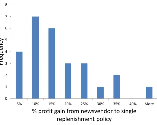
Figure 2.4: Histogram of profit gain with single replenishment, 27 instances, Uniform distri-bution
optimal solutionQ1=Q2=b1+zz. In other words, the optimal policy specifies that the two
ordering decisions are identical, with probability of replenishment 1−F(Q1) =RQb
1
1
b−ad x=
1
b
b−b1+zz=1−(1+zz). However, this does not hold whena >0.
We also consider a numerical analysis of varying problem instances with parameter bounds
listed in Table 2.1.
Table 2.1: Experimental set
low middle high
r , revenue 1.75 2.5 3.25
s , salvage 0 0.4 0.8
p, lost sales penalty 0 0.5 1 c1=c2, materials cost 1
For each problem instance, we compare the expected seasonal profit of a newsvendor
40.00 50.00 60.00 70.00 80.00 90.00 100.00
1 3 5 7 9 11 13 15 17 19 21 23 25 27
O
rd
er
q
ua
nt
ity
27 instances, ordered by newsvendor fractile Single
replenishment No replenishment
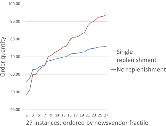
Figure 2.5: Comparing expected total units ordered over, 27 instances, Uniform distribution
analysis,F(ξ)∼U(10, 100). Across these instances, we find the average percentage increase
in seasonal profit by allowing the option of a replenishment to be 15.4%, with a median
improvement of 13.2%. A histogram of the profit improvement is shown in Figure 2.4.
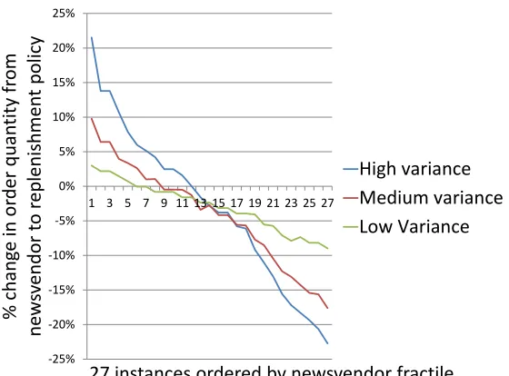
An interesting result is the comparison of total units ordered. For the newsvendor problem
with uniform demand between(a,b), total units ordered is simplya+r+p−c1
r+p−s (b−a). When
a replenishment order opportunity is allowed, the expected number of total units ordered
isQ1+Q2(1−F (Q1)). Numerically, we can find the percent change in total expected units
ordered. These results are summarized in Figure 2.5. The results show that in low service level
cases, the replenishment opportunity results inmoregoods being ordered compared to the
single order newsvendor case. Problem instances with increasing service level show a trend
that the replenishment opportunity “allows” fewer units to be ordered on average comapred
to the newsvendor solution, while still increasing profits and maintaining service levels.
Comparing the newsvendor order quantity withQ1for the replenishment problem, we
find that the average difference over the problem instances tested was 36%. In other words,
Table 2.2: Analysis of variance results
Statistical p–values
% Profit increase % Sales increase % Lost sales decrease
Revenue 0.008 0.013 0.015
Lost sales penalty 0.555 0.604 0.615
Salvage value 0.001 0.0002 3.183e(-5)
average of 36%. IfQ1is depleted in the replenishment case and a subsequent order ofQ2is
made, the average increase in the total units ordered during the season is 13% over the simple
newsvendor order quantity.
We conduct an analysis of variance (ANOVA) test to determine which of the factors are
most important in determining the value of the replenishment opportunity. In addition, we
conduct a similar ANOVA test against the percentage increase in the number of goods sold
with the replenishment opportunity, as well as the percentage decrease in lost sales with the
replenishment opportunity. These results are highlighted in Table 2.2. It is worth noting that
revenue and salvage value were considered significant at the 0.05 significance level, whereas
the lost sales penalty,p, was not. This results stems from the fact that the lost sales penalty is
small compared to the lost revenue of missing a sale. In other words, missing the revenue is
Figure 2.6: ANOVA results for % profit increase with replenishment, salvage value term
Visually, we see in Figure 2.6-Figure 2.14, the same percentage changes as shown