Scholarship@Western
Scholarship@Western
Electronic Thesis and Dissertation Repository
4-15-2016 12:00 AM
Data Smoothing Techniques: Historical and Modern
Data Smoothing Techniques: Historical and Modern
Lori L. Murray
The University of Western Ontario
Supervisor David Bellhouse
The University of Western Ontario Joint Supervisor Duncan Murdoch
The University of Western Ontario
Graduate Program in Statistics and Actuarial Sciences
A thesis submitted in partial fulfillment of the requirements for the degree in Doctor of Philosophy
© Lori L. Murray 2016
Follow this and additional works at: https://ir.lib.uwo.ca/etd
Part of the Statistics and Probability Commons
Recommended Citation Recommended Citation
Murray, Lori L., "Data Smoothing Techniques: Historical and Modern" (2016). Electronic Thesis and Dissertation Repository. 3679.
https://ir.lib.uwo.ca/etd/3679
This Dissertation/Thesis is brought to you for free and open access by Scholarship@Western. It has been accepted for inclusion in Electronic Thesis and Dissertation Repository by an authorized administrator of
Some elementary data smoothing techniques emerged during the eighteenth
cen-tury. At that time, smoothing techniques consisted of simple interpolation of the data
and eventually evolved into more complex modern methods. Some of the significant
milestones of smoothing or graduation of population data will be described including
the smoothing methods of W.F. Sheppard in the early twentieth century. Sheppard’s
statistical interests focused on data smoothing, the construction of mathematical
ta-bles and education. Throughout his career, Sheppard consulted Karl Pearson for
advice pertaining to his statistical research. An examination of his correspondence
to Pearson will be presented and his smoothing methods will be described and
com-pared to modern methods such as local polynomial regression and Bayesian smoothing
models.
In the second part of the thesis, the development of Bayesian smoothing will be
presented and a simulation-based Bayesian model will be implemented using
histori-cal data. The object of the Bayesian model is to predict the probability of life using
grouped mortality data. A Metropolis-Hastings MCMC application will be employed
and the results will then be compared to the original eighteenth-century analysis.
Keywords: Data smoothing methods, smoothing, splines, Bayesian smoothing,
Shep-pard, Pearson, life tables, history of statistics.
I would like to express my sincere thanks to my advisors Dr. David Bellhouse for
his extensive knowledge in the history of probability and statistics and Dr. Duncan
Murdoch for his expertise in statistical computation. I am genuinely grateful to have
had the opportunity to study and research both the historical and modern methods
of statistics with them.
I would also like to thank my husband Jeff and our three children for their love
and support while working on this thesis.
Abstract ii
Acknowlegements iii
List of Figures vi
List of Tables viii
List of Appendices ix
1 Introduction 1
2 The Development of Early Smoothing Techniques 3
2.1 Introduction . . . 3
2.1.1 Graunt’s Life Table . . . 4
2.1.2 Halley’s Life Table . . . 5
2.2 Eighteenth-Century Smoothing . . . 7
2.2.1 De Moivre’s Survival Function . . . 7
2.2.2 Smart’s Life Table . . . 8
2.2.3 Simpson’s Life Table . . . 11
2.2.4 The Northampton Table . . . 12
2.3 Nineteenth-Century Smoothing . . . 14
2.3.1 The Carlisle Table . . . 14
2.3.2 Gompertz-Makeham Law of Mortality . . . 16
2.3.3 The English Table . . . 17
2.4 Early Twentieth-Century Smoothing . . . 18
2.5 Conclusion . . . 19
3 The Correspondence from Sheppard to Pearson 21 3.1 Background . . . 21
3.2 Early Correspondence . . . 22
3.3 Statistical Correspondence . . . 25
3.3.1 Probable Error . . . 27
3.3.2 Corrections of Moment Estimates . . . 30
3.3.3 Methods of Fitting Curves . . . 32
3.3.4 Quadrature Formulae . . . 37
3.3.5 Tests of Fit and Pearson’s Chi-Square Test . . . 38
3.3.6 Numerical Tables . . . 40
3.4 Later Correspondence . . . 41
4 Sheppard’s Tables 43 4.1 Background . . . 43
4.4 How Sheppard’s Tables Were Used . . . 50
5 Sheppard’s Smoothing Methods 53 5.1 Background . . . 53
5.2 Sheppard’s Smoothing Formula in Terms of Central Differences . . . 54
5.3 Sheppard’s Smoothing Formula in Terms of Central Summations . . . 59
5.4 Sheppard’s Smoothing Method Based on the Method of Least Squares . . . 65
5.5 Precursor Methods to Local Polynomial Regression . . . 66
5.6 Comparing Sheppard’s Methods to Modern Methods . . . 67
5.6.1 Local Polynomial Regression . . . 67
5.6.2 Bayesian Smoothing Method . . . 69
5.7 Conclusion . . . 77
6 The Development of Bayesian Smoothing 79 6.1 Background . . . 79
6.2 The Bayesian View . . . 80
6.3 Bayesian Smoothing . . . 81
6.4 Bayesian Smoothing and Mortality Data . . . 82
6.5 Conclusion . . . 84
7 Bayesian Smoothing 85 7.1 The Objective . . . 85
7.2 Preliminary Analysis of the Data . . . 85
7.3 The Model: Bayesian Smoothing . . . 87
7.4 Metropolis-Hastings MCMC . . . 92
7.5 Analysis . . . 93
7.6 Conclusion . . . 103
8 Conclusion 105
References 106
A Smart’s Life Table 115
B Correspondence from
W.F. Sheppard to K. Pearson 117
C Infant Mortality Data 136
Curriculum Vitae 136
2.1 Halley’s estimates of the number of lives at each age. . . 7
2.2 Smart’s estimates (lower curve) and Halley’s estimates of the number of lives at each age. . . 9
2.3 Simpson’s estimates (lower curve) and Halley’s estimates of the number of lives at each age. . . 11
2.4 Carlisle population curve. . . 15
3.1 Pearson’s histogram. . . 34
3.2 Pearson’s diagram of a frequency curve based on observations forming a series of polygons. . . 35
5.1 Sheppard’s smoothed values (open circles) and the data (solid circles) using method of least squares. . . 66
5.2 Differences between the smoothed values using Sheppard’s method and local polynomial regression. . . 69
5.3 Bayesian smoothing model using k=0.1. . . 72
5.4 Bayesian smoothing model using k=1. . . 73
5.5 Bayesian smoothing model using k=5. . . 73
5.6 Bayesian smoothing model using k=10. . . 74
5.7 Residual plot using k=5. . . 74
5.8 The 95% credible intervals using k=5. . . 75
5.9 Comparison of Sheppard’s smoothed values (open circles), Bayesian smooth-ing (line) ussmooth-ing k=5 and the data (solid circles). . . 76
5.10 Differences between Sheppard’s smoothed values and Bayesian μ(t) eval-uated yearly. . . 77
7.1 Cumulative number of deaths per thousand versus age as reported by Smart (open circles) and group data (solid circles). . . 86
7.2 Cubic B-splines on [0,100] corresponding to knots at 0, 2, 5, 10, 20, 30, 40, 50, 60, 70, 80, 90 and 100. . . 88
7.3 Prior samples of λ(t) for k= 0.1, 1, 3 and 10. . . 91
7.4 Trace plots for the last 100,000 iterations for parameters 1 to 15. . . 94
7.5 Trace plots for the last 100,000 iterations for parameters 1 to 15 using different standard deviations. . . 95
7.6 λ(t): number of deaths per year. . . 96
7.7 λ(t) and rectangles representing the area for each age group cell. . . 96
7.8 Standardized residuals for each age group. . . 97
7.9 Trace plots for the last 100,000 iterations for parameters 1 to 15 using step function penalty. . . 98
7.10 Trace plots for the last 100,000 iterations using different standard devia-tions for parameters 1 to 3. . . 99
7.12 λ(t) with 95% credible intervals. . . 100 7.13 Standardized residuals for each age group using step function. . . 101 7.14 λ(t) and rectangles representing the area for each age group starting at
age 2. . . 101 7.15 Hazard function with 95% credible intervals. . . 102 7.16 Comparison of the Bayesian model (line) and Smart’s cumulative
distri-bution (open circles). . . 103
2.1 Graunt’s Life Table. . . 4
2.2 Halley’s Breslau table. . . 6
2.3 Mortality rates from the Bills of Mortality for London, 1728 to 1737. . . 9
2.4 The Construction of the Northampton Table. . . 12
2.5 The Carlisle data. . . 15
3.1 Descriptions of the 23 letters from Sheppard to Pearson. . . 22
4.1 Sheppard’s tables related to the normal curve. . . 47
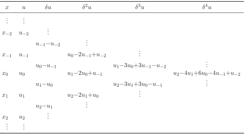
5.1 Central differences of u0. . . 55
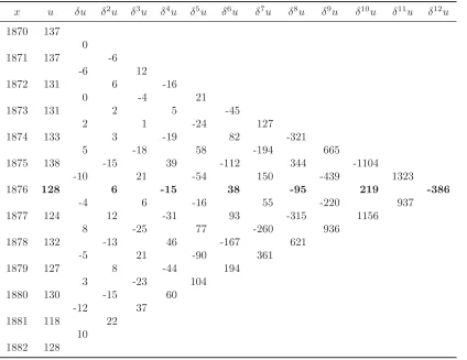
5.2 Central differences of u7 using the infant dataset. . . 58
5.3 Central differences of vi. . . 60
5.4 General form for calculating central sums. . . 60
5.5 Central sums using the infant dataset. . . 62
5.6 Central sums to obtain v1. . . 63
Appendix A: Smart’s Life Table . . . 115 Appendix B: Correspondence from W.F. Sheppard to K. Pearson . . . 117 Appendix C: Infant Mortality Data . . . 136
Introduction
In this thesis, historical and modern data smoothing techniques are presented and
compared. The topics would be of interest to the statistical community and for those
with an interest in the history of statistics.
Chapter 2 describes some of the significant milestones of early smoothing
meth-ods beginning in the late seventeenth century. Some of the earliest evidence of
smooth-ing data can be found in the construction of life tables. Since population data contains
irregularities, some adjusting or smoothing of the data is necessary. The collection of
early data was often grouped by age and the gaps in the ages, such as deaths grouped
into ranges with breaks at ages 10, 20, 30 years and so on, required smoothing for
the purpose of interpolation. Elementary smoothing techniques such as visual
inter-polation, averaging, and mathematical interpolation were used to smooth out such
irregularities in the data.
As the quality of data improved, smoothing methods became more advanced.
Parametric and nonparametric models were developed along with graphical
meth-ods and difference formulas. The smoothing method of W.F. Sheppard in the early
twentieth century was a significant milestone in the development of data smoothing.
Sheppard’s statistical career and correspondence to Karl Pearson are described in
Chapter 3. The correspondence spans three decades and it is obvious they became
very close colleagues and good friends. Although the correspondence is one-sided
(only the letters from Sheppard to Pearson are extant), they provide an
interest-ing background to their statistical ideas and opinions before their manuscripts were
published.
In the letters, Sheppard often asks Pearson for his advice regarding formulas for
the tabulations of his tables related to the normal distribution. These were the first set
of modern tables for the normal distribution based solely on the standard deviation.
Throughout his career, Sheppard increased the accuracy of the tables by obtaining a
higher number of decimals. Chapter 4 describes the methods of construction of his
tables and how they were used.
Sheppard presented his smoothing method in a series of publications from 1912
to 1915. His method involves central differences and summation formulas based on
least squares and is given in Chapter 5. We compare his method to modern smoothing
methods such as local polynomial regression and Bayesian smoothing models.
The development of Bayesian smoothing and applications to the construction of
life tables are given in Chapter 6.
In Chapter 7, a Bayesian smoothing model is developed to predict the probability
of life using eighteenth-century mortality data. The model implements a Metropolis
Hastings MCMC algorithm and the results are compared to the original eighteenth
century analysis.
Chapter 8 provides a conclusion to the thesis. The various smoothing techniques
The Development of Early
Smoothing Techniques
2.1
Introduction
This chapter provides an overview of the development of early smoothing techniques
beginning in the seventeenth century. Some of the earliest evidence of smoothing is
found in the construction of life tables. A life table shows the number of persons
alive at each age, and allows inferences to be made, such as the probability of
sur-viving any particular age or the remaining life expectancy for persons at different
ages. Population data contain irregularities and some adjusting or smoothing of the
data is necessary in order to obtain reasonable estimates. The collection of detailed
population data was slow to evolve. With the absence of a population census, early
life tables were constructed from a limited number of observations spanning a short
period of time. The compilers of early life tables did not disclose their exact methods
of construction. However, given the techniques that were available to them at the
time and examining others who used their methods, possible methods of construction
will be described.
2.1.1
Graunt’s Life Table
John Graunt, a London merchant, constructed a life table based on the observations
recorded in the Bills of Mortality for the City of London, England. Starting in the
early seventeenth century, the Bills of Mortality were bulletins published weekly to
show the number deaths to warn residents of possible outbreaks of the bubonic plague.
The London Bills consisted of the number of baptisms and deaths collected from parish
clerks. As the main concern was for risk of recurrent epidemic diseases, only the cause
of death was recorded and not the age at which a person died. Information about the
collection and publication of these data can be found in “London Plague Statistics
in 1665” (Bellhouse 1998). Using the London Bills, Graunt estimated the number of
births and the number of persons living up to age 6, 16, and for every ten years up
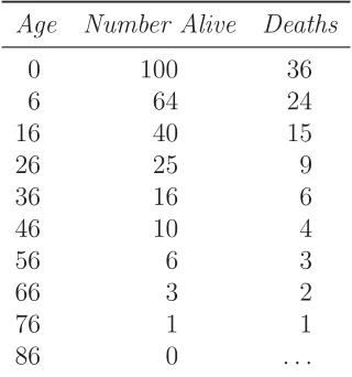
to age 86. He determined that for every 100 births, 36 die before the age of 6. Since
the data was not grouped by age, Graunt had to guess the ages at which people had
died given the cause of death. The results were published in 1662 in “National and
political observations made upon the Bills of Mortality” (Graunt 1662) and are shown
in Figure 2.1.
Table 2.1: Graunt’s Life Table.
Age Number Alive Deaths
0 100 36
6 64 24
16 40 15
26 25 9
36 16 6
46 10 4
56 6 3
66 3 2
76 1 1
86 0 . . .
We observe a smooth progression after age 6 where the number of persons living is
rate of about 95.4%, independent of age. The annual mortality rate according to
Graunt’s estimates would then be 1/18. The overall annual mortality rate shown
in his data is 1/27 (Lewin and Valois 2003). Perhaps if Graunt had realized the
discrepancy he would have adjusted the adult mortality rates to increase with age
making the estimates in his table more accurate.
2.1.2
Halley’s Life Table
Nearly thirty years later in 1693, Edmond Halley designed a life table based on
mor-tality data for the valuation of life annuities. Casper Neumann, a Protestant pastor,
collected the data from the parish registers in Breslau from 1687 to 1691. The city of
Breslau in Silesia is now called Wroclaw in Poland. The data consist of the number of
births and the number of deaths including the age at which people had died. Halley
obtained the Breslau data, analysed it and constructed a life table. The Breslau data
show that the population was approximately stationary. A stationary population is
when the number of births equal the number of deaths and the age-specific mortality
rates remain constant over time.
Analysing the data, Halley determined that the total population of Breslau was
approximately 34,000 with a mean of 1238 births per year and 348 deaths in the first
year of life. This gives (1238 + (1238-348))/2 = 1064, the mean number of infants
alive in the first year. Halley rounded this number to start his population table
with 1000 persons alive in the first year of age. Bellhouse (2011) illustrates how the
additional 64 lives were redistributed throughout the early years of life. Halley’s table
is referred to as a life table, although by correct definition, it is a population table
since it displays the mean number of persons alive at each age for Breslau (Greenwood
1941).
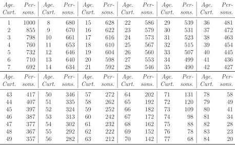
Table 2.2 shows Halley’s estimates of the number of persons living at each age
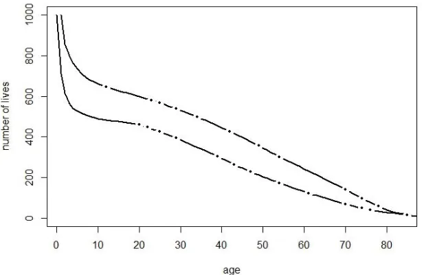
reached their birthday of that year. Figure 2.1 show Halley’s estimates of the number
of persons alive as a function of age. Smoothing was necessary due to the irregularities
of the data and the small numbers of deaths at the older ages. Calculating the slope
for the yearly rates we find that Halley used piecewise linear interpolation to smooth
out such irregularities. In general, Halley’s estimates are approximately linear from
age 12 to 78. The curve in Figure 2.1 is exactly linear between the dots.
Table 2.2: Halley’s Breslau table.
Age. Per- Age. Per- Age. Per- Age. Per- Age. Per- Age. Per-Curt. sons. Curt. sons. Curt. sons. Curt. sons. Curt. sons. Curt. sons.
1 1000 8 680 15 628 22 586 29 539 36 481
2 855 9 670 16 622 23 579 30 531 37 472
3 798 10 661 17 616 24 573 31 523 38 463
4 760 11 653 18 610 25 567 32 515 39 454
5 732 12 646 19 604 26 560 33 507 40 445
6 710 13 640 20 598 27 553 34 499 41 436
7 692 14 634 21 592 28 546 35 490 42 427
Age. Per- Age. Per- Age. Per- Age. Per- Age. Per- Age. Per-Curt. sons. Curt. sons. Curt. sons. Curt. sons. Curt. sons. Curt. sons.
43 417 50 346 57 272 64 202 71 131 78 58
44 407 51 335 58 262 65 192 72 120 79 49
45 397 52 324 59 252 66 182 73 109 80 41
46 387 53 313 60 242 67 172 74 98 81 34
47 377 54 302 61 232 68 162 75 88 82 28
48 367 55 292 62 222 69 152 76 78 83 23
49 357 56 282 63 212 70 142 77 68 84 20
The results were published in 1693 in Philosophical Transactions titled “An
es-timate of the degrees of the mortality of mankind, drawn from curious tables of the
births and funerals at the City of Breslaw; with an attempt to ascertain the price of
annuities upon lives” (Halley 1693). The table proved to be reliable in the valuation of
annuities. Halley’s table is considered the world’s first life table and has been analysed
Figure 2.1: Halley’s estimates of the number of lives at each age.
In the eighteenth century Halley’s table was used as a source for other works
such as Daniel Bernoulli’s model on smallpox. Bernoulli used Halley’s table in his
calculations to model the probability of dying of smallpox. Adjusting the number of
births from 1238 to 1300 was the only change Bernoulli made to Halley’s estimates
(Baca¨er 2011, pp. 21–29).
2.2
Eighteenth-Century Smoothing
2.2.1
De Moivre’s Survival Function
Deriving estimates for annuities using Halley’s life table was a laborious task. In 1725
Abraham De Moivre developed a survival function that simplified the calculations.
De Moivre used the fact that Halley’s table was approximately linear after age 30 and
used this assumption in deriving his survival probability model (De Moivre 1725).
annuities of joint lives as a function of the corresponding annuities on single lives,
De Moivre used an exponentially decreasing function. The two assumptions, linear
and exponential, are incompatible but De Moivre did it anyway to obtain a simple
approximation (Bellhouse 2011b, pp. 161–164).
2.2.2
Smart’s Life Table
Nearly 65 years after the publication of Graunt’s life table, the collection of mortality
data in London remained unchanged; parish clerks were required to report only the
cause of death and not the age at which a person had died. In 1726 John Smart,
a clerk at Guildhall London, wanted to construct a life table to estimate annuities
but his design required the number of deaths at each age with observations taken
over several years. Smart describes the problem in his book titled “Tables of Interest,
Discount, Annuities, &c” (1726, p. 113). Smart didn’t feel a change would be made
during his lifetime. However, in less than two years after the publication of his book,
parish clerks were required to include the approximate age of death. By 1737 Smart
felt he had enough observations to construct a life table for the City of London.
Smart’s life table along with the raw data is recorded on a broadside and held
in the Guildhall Library in London (Smart 1738b). Extracted from the London Bills,
the data gives the number of deaths for each year between 1728 to 1737 inclusive
for each age group ranging from birth to greater than 90. Table 2.3 shows the total
number of deaths for each age group and the corresponding number out of 1000.
Smart took the total number of deaths over ten years for each age group and
determined the proportion out of 1000. We find from Smart’s life table in Appendix A
that the yearly rates remain constant over a few years. Smart retained the proportion
of death for each age group given in the data and used piecewise linear interpolation
to obtain the number of lives and deaths for the years between each age group.
Table 2.3: Mortality rates from the Bills of Mortality for London, 1728 to 1737.
Age Group Total Deaths Out of 1000
0 to 2 103159 386
2 to 5 23505 88
5 to 10 9775 36
10 to 20 8242 31
20 to 30 19776 74
30 to 40 24302 91
40 to 50 23989 90
50 to 60 19693 74
60 to 70 16309 61
70 to 80 10684 40
80 to 90 6450 24
> 90 1266 5
for Breslau (upper curve). Smart estimates higher mortality rates than Halley’s except
for the older ages. Calculating the slope for the yearly rates we find Smart’s curve
is approximately linear from age 21 to 71. From age 21 to 60 the curves are nearly
parallel. The curves are exactly linear between the dots.
Smart wrote a letter to George Heathcote and enclosed a copy of his table
es-timates (Smart 1738a). Heathcote was a politician and a member of parliament in
London. Dated February 25th, 1737, Smart explains to Heathcote how his life table
is different than Halley’s. Smart writes
. . . you will find a very great Difference more especially in the early part
of Life. For 1238 Persons dying yearly at Breslau, the Doctor computes
616 of them, which is near one half, attain the age of seventeen: whereas
by my Table, of 1000 Persons, there are but 501 who live to eight years
of Age. But with respect to old Age, the Tables agree well enough for, by
the one, 20 of the 1238, live to eighty four; by the other, 20 in 1000, to
eighty three years of Age. (Smart 1738a)
Smart also explains how the two cities are different:
. . . Breslau is an inland City in Germany, inhabited chiefly by sober,
in-dustrious Peoples, Strangers to Luxury that Parent of all Vices, whereas
London is a City abounding with Luxury amongst the Rich, and
Debauch-ery amongst both of the Rich and Poor. (Smart 1738a)
Smart acknowledges that Breslau and London are different, but like Halley’s table
he assumed the population of London was stationary when he constructed the table.
A consequence of assuming a stationary population is that the characteristics of the
population are independent of time. This means that for each age group the number
of live persons is always the same as that of the original life table. This is not realistic
since most populations vary over time. A life table constructed with this assumption
does not guarantee accurate estimates in the long run. The assumption was not
practical for the city of London as it was with Breslau. At the time, London was
experiencing significant immigration. Smart’s estimates were based on the number of
births, the number of deaths, and the age of death. He did not know the number of
2.2.3
Simpson’s Life Table
The consequence of Smart’s assumption of a stationary population was quickly
rec-ognized by Thomas Simpson. Simpson (1742) published a revision to Smart’s table
that tried to take into account migration. Simpson changed Smart’s estimates up to
age 25 and kept the remaining estimates the same. Simpson increased the number
of births from 1000 to 1280, and using Halley’s life table as a reference, used linear
interpolation for the younger ages (Hald 1990, pp. 518–519). Figure 2.3 shows
Simp-son’s estimates (lower curve) and Halley’s estimates (upper curve) for the number of
lives at each age. Simpson estimates higher mortality rates than Halley except for
the older ages. Calculating the slope for the yearly rates we find Simpson’s curve is
approximately linear after age 12. The curves are nearly parallel from age 12 to 60.
The curves are exactly linear between dots. Simpson’s table was published in 1742
and used for insurance purposes (Hald 1990, p. 519).
2.2.4
The Northampton Table
Mathematician, philosopher and theologian Richard Price constructed a life table
based on observations from the Register of Mortality at Northampton. The data are
from the burial register of the Parish of All Saints in Northampton, England and
spans 46 years from 1735 to 1780. The first version of the table was compiled using
data from 1735 to 1770. With ten additional years of data in hand, Price revised
and published the table in 1783 in Observations reversionary payments; schemes
for providing annuities for widows, and for persons in old age; on the method of
calculating the values of assurances on lives. The data consist of 4689 deaths and 4220
baptisms, a difference of 469 (or 10%). Price describes his method of construction on
page 358 of hisObservationsalthough he is not explicit. William Farr (1848) explains
in the 8th Report of the Registrar General that Price accounted for immigration at
age 20. Based on Farr’s description, W. Sutton (1883) proposes a method for the
construction of the table. The construction of Price’s life table is shown in Table 2.4.
Table 2.4: The Construction of the Northampton Table.
(1) (2) (3) (4) (5) (6) (7) (8)
Age Deaths Deaths Living Living Less 1300 Living Northampton Adjusted 10000 under 20 Adjusted Table
0 1529 1529 4689 10000 8700 11649.2 11650
2 362 362 3160 6739 5439 7283 7283
5 201 201 2798 5967 4667 6249 6249
10 189 189 2597 5538 4238 5675 5675
20 373 351 2408 5135 3835 5135 5132
30 329 351 2057 4387 . . . 4387 4385
40 365 365 1706 3638 . . . 3638 3635
50 384 384 1341 2860 . . . 2860 2857
60 378 378 957 2041 . . . 2041 2038
70 358 358 579 1235 . . . 1235 1232
80 199 199 221 471 . . . 471 469
90 22 22 22 47 . . . 47 46
100 . . . 0 21 . . . 0 0
each age group. For example, there are 1529 deaths from birth up to age 2, and there
are 362 deaths from age 2 up to age 5, and so on. Price smooths the number of deaths
by averaging the age groups 20 to 30 and 30 to 40 so that they are equal (shown in
bold). Column 4 corresponds to the number of person living if the population was
stationary with the initial value for the number of persons alive from birth to age 2
being the sum of all the deaths from column 3. Column 5 is the number of persons
living for each age group proportionally increased for a population size of 10,000.
Column 6 is smoothed to account for immigration by decreasing up to age group 20
to 30 in column 5 by 1300 (13% of 10,000 instead of the 10% suggested by the data).
Column 7 increases the first five age groups by the proportion (5135/3835) required
to restore the age group 20 to 30 to the original value in column 5. The last column
shows Price’s Northampton table. The differences between the last two columns differ
by no more than 3 between the age 20 and 90.
Price’s Northampton table was constructed properly based on the given data
(Registrar General 1848, p. 291). However, Farr (1853) states that the data did not
accurately represent Northampton because there were a great number of Baptists
liv-ing in the town and they do not baptize infants. This reduced the ratio of christenliv-ings
to deaths, which decreased the average life expectancy. The consequence of this was
that the mean duration of life was assumed to be 24 years when it was really about
30 years. The table was used by the Equitable Life Assurance Society and the British
government for 20 years to determine the price of annuities it sold. This led to losses
2.3
Nineteenth-Century Smoothing
2.3.1
The Carlisle Table
Joshua Milne employed a graphical smoothing method in the construction of the
Carlisle Table, a life table based on data from the City of Carlisle. Milne was an
actuary for the Sun Life Assurance Society. The table was published in 1815 in A
Treatise on the Valuation on Annuitities and Assurances on Lives and Survivorships
(Milne 1815). The data were provided by John Heysham, a medical doctor, and was
taken from population data and the Bills of Mortality of two parishes in Carlisle. The
data consist of a census of grouped data for the number of persons living for the years
1780 and 1787. The data include the number of deaths for the same age groups with
birth to 5 given in one year intervals covering the period from 1779 to 1787.
Columns 1 to 3 in Table 2.5 show the data with the number of persons alive for
each age group for the years 1780 and 1787 respectively. The total number of persons
living for the eight-year period is calculated as the sum of the 1780 and 1787 censuses
multipled by 4 and is shown in column 4. Column 5 is the total number of persons
living (column 4) divided by the width of each age group and rounded to the nearest
integer.
Milne begins his graphical approach by constructing rectangles whose base
cor-responds to the widths of each age group and the heights as calculated in column 5
of Table 2.5. For example, the age group birth to 5 has 8772 persons living over a
five year period which represents the area of the first rectangle with the height given
by 8772/5=1754 from column 5. Using his knowledge and experience, Milne drew a
smooth continuous curve through the tops of the rectangles such that any additional
area added to the rectangles was equal to the amount removed. Milne knew to start
the curve high because the infant mortality data showed a high number of deaths in
Table 2.5: The Carlisle data.
(1) (2) (3) (4) (5)
Age Population Population Living 8 year total Group in 1780 in 1787 8 year total at each age
0 to 5 1029 1164 8772 1754
5 to 10 908 1026 7736 1547
10 to 15 715 808 6092 1218
15 to 20 675 763 5752 1150
20 to 30 1328 1501 11316 1132
30 to 40 877 991 7472 747
40 to 50 858 970 7312 731
50 to 60 588 665 5012 501
60 to 70 438 494 3728 373
70 to 80 191 216 1628 163
80 to 90 58 66 496 50
90 to 100 10 11 84 8
100 to 105 2 2 16 . . .
Figure 2.4 is Milne’s graph of the Carlisle population curve (Milne 1815, p. 101).
Milne used the graph for the purpose of illustration but did not include the values for
the horizontal and vertical axes.
The Carlisle table is constructed from the graph in Figure 2.4. The number of
persons living for each year is determined by finding the year on the horizontal axis
and the corresponding value on the curve. The same graphical interpolation method
can be used to find the number of deaths as illustrated by actuary George King (1883).
The Carlisle table was widely adopted by actuaries and used for many years for
the valuation of annuities (BMJ 1902). TheBritish Medical Journal featured Milne’s
method in its 1902 publication concluding that the graphical method “is simpler, more
elegant, and equally accurate with the analytical method” (BMJ 1902).
2.3.2
Gompertz-Makeham Law of Mortality
Mathematician and actuary Benjamin Gompertz derived a parametric model for the
construction of life tables. The idea of the model was first introduced and published
inPhilosophical Transactionsin 1820 and 1825, and further developed and presented
to the Royal Society in 1861 (Gompertz 1820, 1825, 1861). The model is known as
the Law of Mortality. Let Dx be the cumulative number of deaths up to age x, then
Dx =Bcx (2.1)
whereB andcare constants. Fellow actuary William Makeham revised the model to
improve the accuracy. The model was published in theJournal of the Institute of
Ac-tuaries in 1859 titled “On the Further Development of Gompertz’s Law”. Makeham’s
model includes the addition of a constant term A and is given by
Dx =A+Bcx. (2.2)
The model is useful for smoothing mortality observations and for calculating the value
2.3.3
The English Table
Farr constructed the first four English Life Tables. The third life table was published
in 1864 and the method for its construction is described in full in his book, English
Life Table(Farr 1864). The data are based on the 1841 and 1851 population censuses
for England and Wales and the number of deaths for the 17 years from 1838 to 1854
for both males and females from the civil registrations. The data consist of population
and deaths for individual years from birth to age 4, for every five years up to age 15,
and for every ten years up to greater than 95 (Farr 1864, p. xix).
Farr obtained a uniform distribution of deaths using
px =
2−mx
2 +mx
(2.3)
where px is the probability that someone age x will survive to age x+ 1 and mx is
the number of persons dying at age x divided by the mean population at age x. In
other words, mx is the rate at which people are dying in the middle of the year of age
x to x+ 1 and is formally known as the central force of mortality. Farr retained the
rates of mortality for ages under 5 given in the data. For the 10-year groups Equation
(2.3) gives the force of mortality for integral ages instead of for the mean of the year
of age.
Farr assumed that the force of mortality (instantaneous mortality rate at agex)
for a country increased in a geometrical progression using the relation μx+t = rtμx
for t years and r10 =μx+ 10/μx. Then
−ln(px) =
1
0
μt+1dt= r−1
ln(r)μx. (2.4)
Transforming into common logarithms we have
−log(px) = k
2(r−1)
where k = log10e. The values for log(px) for ages 3, 4, 7, 12 and every ten years
thereafter were used as the basis for third difference interpolation after dividing the
table into sections. Table divisions were done separately for males and females based
on the analysis of the data. Farr (1864, p. clxvii) obtained the deaths rates for
each year of life and tabulated the results. The yearly mortality rates are given
in logarithms for both male and female from birth to age 109. The computations
involved were extensive and the tables were used for insurance purposes.
2.4
Early Twentieth-Century Smoothing
A special edition on data smoothing methods was published in 1921,Tracts for
Com-puters by E.C. Rhodes and edited by Karl Pearson. This rare publication examines
and compares some of the data smoothing (or graduation) techniques in use at the
time and served in part as the motivation for this thesis. A large amount of
experi-mental and observational data were collected during W.W.I, which prompted serious
discussion on smoothing methods (Rhodes 1921, p. 4). The staff of the Galton
Lab-oratory, UCL were engaged in research for the Admiralty Air Department and
Min-istry of Munitions and the collection of wartime data was related to fuses, elasticity,
propellers, aircraft and ballistics trajectories, and range tables (Galton Laboratory
Wartime Research Papers, UCL Special Collections, Pearson/9). The smoothing
methods of John Spencer (1904), W.S.B. Woolhouse (1869), A. Cauchy (1837), T.
Sprague (1886) and W.F. Sheppard (1914b) are considered. Spencer’s graduation
formula, also known as the summation formula, uses 15 or 21 values tabulated in
order to obtain one smoothed value at a time. The process is repeated with the series
of smoothed values proceeding by constant third differences. The method is simple
for practical use and was widely used by actuaries. Woolhouse’s method uses 15
val-ues to smooth out the central value, using repeated summations until each value is
smoothed. He was the first person to use differences to smooth data. His method
interpolation. Cauchy suggests a method of smoothing observations using a known
function, and Sprague uses a graphical approach using osculatory interpolation which
requires previous knowledge and experience of the given data.
Great attention is given to Sheppard’s smoothing method using differences based
on least squares. His method is proven to perform well by having the smallest or
same magnitude of mean square error as the other methods studied in the tract.
Sheppard’s statistical career and correspondence to Pearson is given in Chapters 3,
the construction of his tables in Chapter 4, and his smoothing method in Chapter 5.
2.5
Conclusion
The collection of detailed population data increased and was recorded over longer
periods of time. Elementary smoothing techniques evolved into more complex modern
methods. The progression of smoothing methods began with visual interpolation,
averaging, and mathematical interpolation, and developed into smoothing methods
using parametric and nonparametric models, differences and graphical methods. The
motivation for developing new methods or improving on existing ones is to find a way
to adjust the data that results with smoothed values that are closer to the true values,
and thus reducing the error, while keeping in mind that the new method is suitable
for practical use.
Advanced smoothing methods are employed in the construction of modern life
tables. For example, the construction of life tables in use by Statistics Canada (2015)
involve two methodologies: logistic models and splines. B-splines are used for
smooth-ing the ages of death due to their flexibility. The logistic model replaced the quadratic
model in 2005. Studies show that the mortality rate in countries with higher
qual-ity data tended to follow a logistic curve (Statistics Canada 2015). The process of
The Correspondence from
Sheppard to Pearson
3.1
Background
William Fleetwood Sheppard was born in 1863 in Sydney, Australia. He attended
grammar school in Brisbane and was sent to England to finish his education at
Char-terhouse School. He won a scholarship to Trinity College, Cambridge and was Senior
Wrangler in the Mathematical Tripos of 1884. Sheppard became a Fellow of Trinity
College and published a paper on Bessel functions (Sheppard 1889). Sheppard left
Cambridge to pursue a career in law but returned to his interest in education and
research, and focused on statistics. In 1896, he was appointed Junior Examiner in the
Education Department and later promoted to Assistant Secretary. He retired in 1921
at the age of 58. He then became a Senior Examiner at the Univeristy of London
before moving to Edinburgh in 1926. He worked at the Edinburgh University and
was elected a Fellow of the Royal Society of Edinburgh in 1932 (Sheppard 1938).
3.2
Early Correspondence
At the beginning of his statistical career, Sheppard consulted British statistician Karl
Pearson, a leading pioneer of modern statistics who could provide Sheppard with
statistical advice and expertise. Sheppard wrote a letter to Pearson describing a
manuscript he was working on with Francis Galton and asked if he would review it
when it was completed. This was the first letter of a series of 23 letters that are
archived at University College, London (Pearson 1896–1926). The letters have been
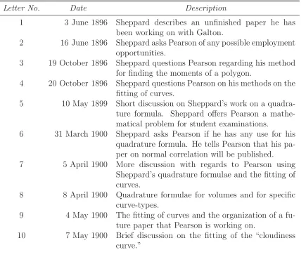
transcribed and can be found in Appendix B. For reference, a brief description of the
letters are given in Table 3.1.
Table 3.1: Descriptions of the 23 letters from Sheppard to Pearson.
Letter No. Date Description
1 3 June 1896 Sheppard describes an unfinished paper he has
been working on with Galton.
2 16 June 1896 Sheppard asks Pearson of any possible employment
opportunities.
3 19 October 1896 Sheppard questions Pearson regarding his method for finding the moments of a polygon.
4 20 October 1896 Sheppard questions Pearson on his methods on the fitting of curves.
5 10 May 1899 Short discussion on Sheppard’s work on a
quadra-ture formula. Sheppard offers Pearson a mathe-matical problem for student examinations.
6 31 March 1900 Sheppard asks Pearson if he has any use for his
quadrature formula. He tells Pearson that his pa-per on normal correlation will be published.
7 5 April 1900 More discussion with regards to Pearson using
Sheppard’s quadrature formulae and the fitting of curves.
8 8 April 1900 Quadrature formulae for volumes and for specific
curve-types.
9 4 May 1900 The fitting of curves and the organization of a
fu-ture paper that Pearson is working on.
10 7 May 1900 Brief discussion on the fitting of the “cloudiness
11 18 December 1900 Sheppard tells Pearson he would like to write a short article about interpolation formulae for sur-faces.
12 13 Febrary 1901 Sheppard encourages Pearson to write an article on the mathematical treatment of statistics for the Times.
13 16 February 1902 Discussion as to where Sheppard’s tables related to the normal distribution could be published. Per-sonal writing about Pearson’s health.
14 13 February 1908 Sheppard asks Pearson the proper etiquette for re-using questions from others’ examination papers in textbooks.
15 18 May 1911 Sheppard discusses a problem on probability. 16 4 October 1911 Sheppard’s tables related to the normal
distribu-tion including a table of values.
17 23 July 1915 Personal topics regarding Sheppard’s family and the health of his eldest son.
18 18 October 1916 Brief discussion about a probability problem. 19 10 April 1925 Brief discussion about Sheppard’s tables related
to the normal distribution with some calculated values.
20 6 September 1925 Discussion about Sheppard’s tables related to the normal distribution and extending the number of decimal places.
21 26 November 1925 More discussion about Sheppard’s tables with some calculated values.
22 2 December 1925 Sheppard desribes 3 of his tables and includes them in the letter.
23 29 June 1926 Details on Sheppard’s tables related to the normal distribution. A personal note on Pearson’s opera-tion.
The letters span three decades from 3 June 1896 to 29 June 1926. The majority
of the correspondence spans the first decade during which time many of Sheppard’s
papers were published. The letters begin very formally with “Dear Sir” and discussions
about statistical methods, but over the course of the thirty years they become informal
where Sheppard speaks of his family and of Pearson’s health. It is obvious that they
became very good colleagues and good friends.
with the hope of being published. He shares his statistical ideas and methods with
Pearson and frequently asks for his advice on which journal would be the most suitable
for the publication of his manuscripts. Reducing the costs of publishing his methods
and tables was also considered. For example, Sheppard suggests using the derivatives
of a function instead of the differences for his tables to save time and space. Sheppard
estimated his quadrature formula would take up 10 or 11 pages using octavo-sized
paper. The speed of the calculations are discussed throughout the correspondence.
Sheppard knew how many minutes it would take to use his method of interpolation
using a Brunsviga mechanical calculator that he had on loan from the Royal Society.
Sheppard wondered if Charles Vernon Boys, a British physicist and inventor, could
devise a machine to simplify the process of calculating large numerical determinants.
Vernon Boys (1944) designed and constructed an integration machine. Instruments,
such as a planimeter were used for testing what Sheppard called “closeness of fit.” A
planimeter determines the area of a two-dimensional shape.
Sheppard was also interested in teaching. He asks Pearson of any possible
em-ployment opportunities and the average hourly rate for private mathematical
coach-ing. In the early correspondence, Pearson offered Sheppard a position to teach
as-tronomy. However, Sheppard declined stating it wasn’t the best subject for him when
he attended Cambridge. Sheppard knew that Pearson set examinations and offered
a problem that he could use in his examinations. He asks Pearson if questions from
publications are allowed to be used in student examinations. The correspondence
shows the solutions to probability questions that Sheppard had worked out for future
examinations.
The letters suggest that Pearson had a major influence on Sheppard’s statistical
work. Sheppard compares his methods and results to Pearson’s in a non-competitative
way to try to fully understand the statistical concepts. For example, Sheppard
dis-covered that Pearson had published a paper on the normal correlation based on the
for normal correlation for the double integral (the bivariate normal distribution) and
found that his method was different than Pearson’s. Sheppard did not always agree
with Pearson’s methods and would offer an explanation as to why. Sometimes he
would give an alternate method and ask for Pearson’s opinion. Sheppard shared
proofs and formulas and referenced Pearson in his published works. Pearson must
have liked Sheppard’s results. He referenced Sheppard’s methods and formulas such
as his corrections of moment estimates for normally grouped data and his
quadra-ture formulas in his own published works (Pearson 1902, 1914a, 1914b). Details of
Pearson’s references will be given later in this chapter.
The letters provide a rare and insightful glimpse into the personal and
profes-sional relationship between Sheppard and Pearson. They give some of the background
details of Sheppard’s methods and formulas that would eventually be published and
adopted by other statisticians.
3.3
Statistical Correspondence
The main theme of their correspondence was the fitting of curves but they also
dis-cussed probable error formulas, moment estimates and corrections to moment
esti-mates for grouped normal data, quadrature formulas, tests of fit, Pearson’s chi-square
test, and tables for the normal density function.
Before proceeding to the specific topics discussed in the correspondence, it is
important to describe some of the statistical terminology and theory that was being
developed at the time. Towards the end of the nineteenth century, asymmetrical
distributions were becoming accepted and new distributions were being developed to
model skewed data. Previously, it was assumed that all continuous statistical data
were normally distributed. Probability distribution functions were called frequency
distributions or curves of frequency. In 1895, Pearson developed four types of
curves had increased to twelve and they became well known as the “Pearson Family
of Frequency Curves” (Stigler 2008). The details of how Pearson derived his family
of curves can be found in §2.3.3. Although they were referred to as parameters, the
constants of the frequency curves were not parameters in the way we define them
today. Quantities such as the mean and standard deviation were expressed, when
possible, in terms of the frequency constants.
Pearson sometimes used the constants of his frequency curves as though they
were parameters but this proved to be consequential. Historian Stephen Stigler (2008)
explains why. Referring to an 1898 paper jointly authored by Pearson and colleague
L.N.G. Filon (Pearson and Filon 1898), Stigler describes a major error when they
incorrectly derived an asymptotically approximate multivariate normal distribution
for the errors of estimation from the expansion of a log-likelihood ratio. The source
of the error was the substitution of integrals for sums in the Taylor expansion. Stigler
points out this was equivalent to replacing the sums with expectations. The Taylor
expansion they used was about the estimates meaning the expectations were then
functions of the estimates and not that of the true values. In other words, there
was no distinction between the estimates and the parameters of the model. Stigler
explains the consequence of the error:
All the expectations are computed as if the estimated values were true
values, and the result is a distribution for errors that does not in any way
depend upon the method used to estimate. (Stigler 2008)
Unfortunately, Pearson lacked the notion of a distribution of true values of the
pa-rameters and “for him there was no ‘true value,’ only a summary estimate in terms
of observed values” (Stigler 2008). At the time, the consequences of the method
went unnoticed. The idea of parametric modelling was not introduced until 1922 by
R.A. Fisher. Fisher presented a method for fitting curves using maximum likelihood
estimation. The new method proved to be superior to Pearson’s method since the
asymptotically normal.
3.3.1
Probable Error
The first letter in the Pearson Papers collection describes an unfinished paper on the
normal curve that Sheppard and Galton had been working on. Sheppard explains
how the paper is entirely theoretical and geometrical without the use of any
differen-tiation or integration. The paper contains new material on the correlation between
normal distributions and that non-normal distributions would only be considered for
the purpose of analysing them into component normal distributions. Sheppard writes
that the paper takes up a great deal of space but he wanted to treat the subject
thor-oughly. Sheppard wanted to know if Pearson would be willing to look at the paper
when it was finished and if he might suggest a suitable journal for its publication.
Sheppard wondered if the paper had a chance of being published in thePhilosophical
Transactions. Given the date of the letter and the subject of the unfinished paper,
it appears Sheppard was referring to his paper, “On the geometrical treatment of
the ‘normal curve’ of statistics,” dated October 1897 and published in the
Proceed-ings of the Royal Society of London (Sheppard 1897b). The paper was revised and
republished under the title, “On the application of the theory of error to cases of
normal distributions and normal correlations,” in 1899 in Philosophical Transactions
of the Royal Society (Sheppard 1899c). In the paper, Sheppard makes reference to
Galton, highlighting his contribution on normal correlation. Sheppard includes his
proof of a theorem in bivariate normal correlation, which is now sometimes known as
Sheppard’s theorem on median dichotomy (MacKenzie 1981, p. 97). In addition, the
paper includes methods for evaluating probable error for the frequency constants of
the normal distribution and tables for calculating probable error.
The term “probable error” was first used in the early nineteenth century to
describe what we now call the median error of an estimate (Stigler 2008). If m
m = 0.6745σ. The first and third quantiles of a normal distribution are 0.6745σ
from the mean. The probability that a deviation is greater than the probable error
is 0.5 and is equal to the probability of a deviation less than the probable error. If
the observed deviation is less than 3 times the standard error it is approximately
equivalent to the observed deviation being less than 4.5 times the probable error.
In his 1899c paper, Sheppard gives two applications where probable error can be
used: for computing the discrepancy between the observed values and the true values,
and for hypothesis tests. The hypothesis tests include the test for normality, test for
normal correlation and the test for independence of two distributions. Generally
speaking, for about half the values of X, the discrepancy, d, should be less than the
probable discrepancy, q, and amongst the remaining values the discrepancy should
not be a large multiple of the probable discrepancy. The ratios,d/q, are computed to
determine if they are or are not greater than we might reasonably expect. Sheppard
includes a table of values to compare with the computed ratio values. The method is
similar to the rejection region approach for hypothesis tests that is used today. Let q
be the quartile deviation (probable discrepancy) andmthe number of random values.
If the area of the standard normal distribution between the pointsx=−p/q andx=
+p/qisφ, then the probability of at least one of the values ofδ being greater thanpis
1−φ. Ifφis chosen such that the probability is 0.5, the corresponding value pwill be
the “probable limit” ofδ. The tables gives 20 values formcorresponding to the values
of the ratio p/q. For example, when m=1 then p/q=1 and when m=10, p/q=2.716.
For values greater than m=20, Sheppard (1899, p. 123) suggests using Chauvenet’s
criterion for the rejection of one out ofm/ln(4+1/2) observations. William Chauvenet
was an American mathematician and astronomer.
Sheppard gives several examples to illustrate the hypothesis tests using probable
error. For example, a hypothesis test to determine if a distribution is normal is given
using grouped data of the chest measurements of 5,732 local Scottish militia, a famous
first step is to calculate the mean ¯x, and standard deviation s. Sheppard (1897a)
uses a special formula to calculate the standard deviation based on grouped data that
he derived in a previous paper. He uses areas to derive the variance which he calls
the mean square and is similar to the shortcut formula we use today to calculate
the variance for grouped data [(f x2)−((f x))2/n)]/(n−1) where f is the group
frequency. This was Sheppard’s first published paper in statistics where he developed
corrections to moment estimates for normally grouped data. Details about the paper
can be found in §3.2.2.
In the next step, Sheppard creates new bins of the chest measurements to equal
the midpoint of each class, for example, 33 belongs to the bin 32.5 to 33.5 and 48
belongs to the bin 47.5 to 48.5. He then computes the class-index, αi, for each value
which represents the standardized proportion for each class [(2ni/n)−1] where ni =
i
j=1fj. The middle ten values (35.5 to 44.5) are standardized, zk for k = 1, . . .10. Sheppard then calculates ¯x+szk for each class k. The discrepancy values,dk, are the
differences between each midpoint value and ¯x+szk. Letφ(zk) be the standard normal
pdf evaluated for each class k, then the standard deviation for each discrepancy is
[s2(1−αk2)/4φ(zk)2 −(1 + 12zk2)]1/2/√n, which when multiplied by 0.67449 gives the
probable discrepancy valuesqk. For the ten classes, four of the actual discrepancies are
less than the probable discrepancies, and the remaining six are greater. In addition,
the ratios (d/q)k are compared to Sheppard’s probable limit δ, mentioned above, for
m=10. Nine of the ten values are less than the corresponding p/q, and therefore, it
is concluded that the data appear to justify the hypothesis of a normal distribution.
The probable error can be calculated using Table V on pages 159 to 166 of
Sheppard’s 1899c paper. The tables contain values for the mean square (variance),
denoted by N, and the intermediate values (shown in the table between two values
of N) that correspond to the probable values, Q√N, where Q=0.67448975... For
example, if the variance is calculated as N= 0.019300, then the value of Q√N to
At the time, probable error was used as a measure of the variability of the
con-stants of frequency curves resulting from a random sample. In this case, the probable
error is the standard deviation of the constant multiplied by 0.67449. The convention
of using probable error as a measure of goodness of the sample, rather than the
stan-dard deviation, was adopted since the theory was developed from the normal curve.
At the end of the first letter, Sheppard wrote a post script stating he “should be
much gratified if any of my work would be of use to you in your own investigations.”
In their 1898 paper, Pearson and Filon derived the probable error for the frequency
constants but used a different method than Sheppard (Pearson and Filon 1898). They
used a Bayesian approach with a uniform prior, which was sometimes referred to as
the Gaussian method (Stigler 2008, p. 5). It was a method of inverse probability
and was commonly used over the nineteenth century. As noted by Stigler, Pearson
and Filon’s derivations contained some errors in the distinction between the estimates
and the population parameters. Over time, Pearson distanced himself from his
prob-able error methods in preference for Sheppard’s non-Bayesian methods (MacKenzie
1981, pp. 203-204) and (Stigler 2008). Pearson referenced Sheppard as being the
“fundamental memoirs on the subject” in the editorial appearing in the volume of his
1903 paper titledOn the probable error of frequency constants (Pearson 1903, p. 35).
Pearson included Sheppard’s methods for finding the probable error of the frequency
constants for five types of his system of curves. Sheppard’s methods for evaluating the
probable error for the frequency constants involve simple linear functions of frequency
counts using a Taylor expansion when necessary. The probable errors are estimated
and then the moments are found from the variances and covariances of the counts.
3.3.2
Corrections of Moment Estimates
The early correspondence includes references to methods for finding moment
esti-mates. In Letter 3, Sheppard enclosed a manuscript for Pearson to review, suggesting
put the mathematical part into a separate paper and asks for Pearson’s advice on
the possibility of it being published in the Philosophical Magazine or the Cambridge
Philosophical Society. It appears Sheppard is referring to his first statistical paper
published in 1897 in the Journal of the Royal Statistical Society (Sheppard 1897a).
The paper summarizes his corrections of moment estimates for normally grouped
data. They were fully presented mathematically in 1898 (Sheppard 1898) and
be-came known as “Sheppard’s corrections” (Aitken 1938).
For continuous frequency distributions, it can be assumed frequencies are
cen-tered at the midpoints of the class intervals when calculating the moments. This
introduces some error and corrections are required. In modern notation, letμn be the
nth central moment, μ∗n the corresponding corrected moment and c the bin width.
Sheppard’s first five corrected moments are:
μ∗1 =μ1 = 0
μ∗2 =μ2 − 1
12c
2
μ∗3 =μ3
μ∗4 =μ4 −1
2μ2c
2+ 7
240c
4
μ∗5 =μ5 −5
6μ3c
2
In a memoir, after Sheppard’s death, A.C. Aitken highlights an error where
Pearson incorrectly omits the use of the corrections in his 1895 paper (Pearson 1895).
Aitken writes that corrections of the moment estimates should be applied in a certain
case for grouped data and gives Sheppard credit for deriving them (Aitken 1938).
Aitken describes how Sheppard was tactful in pointing out Pearson’s error and because
of this, his corrections were not universally adopted for some time.
Pearson used Sheppard’s corrections of moment estimates throughout his 1902
paper, “On the Systematic Fitting of Curves to Observations and Measurements”
Tables for Statisticians and Biometricians, a publication edited by Pearson (Pearson
1914a, 1914b). The first four moments are calculated on the head circumferences
of 1,306 criminals. The data consist of 40 sub-groups and Pearson suggests that 20
sub-groups be used instead, and that Sheppard’s corrections would fully adjust for
the difference (Pearson 1914a, p. lxxvi).
3.3.3
Methods of Fitting Curves
Differences in their statistical views and methods began to surface a few months
into their correspondence. Two back-to-back letters (Letters 3 and 4) reveal some
of these differences. In Letter 3, Sheppard informs Pearson that after reading his
essay on “Skew Variation”, he modified a manuscript he was working on to include a
reference to Pearson’s paper and for illustration to include one of his tables. Sheppard
(1898) was working on his manuscript on corrections of moment estimates which
includes an appendix on the moments of a polygon based on a frequency curve. In
the letter, Sheppard writes that his method for finding the moments of a polygon
based on observations is very different from Pearson’s and that his method “seems
the more correct.” This would have been of interest to Pearson since the moments of
a polygon based on observations were used in his method for fitting frequency curves
to data. Sheppard is referring to Pearson’s 1885 paper titled, “Contributions to the
Mathematical Theory of Evolution. II. Skew Variation in Homogeneous Material”
(Pearson 1895). Pearson’s essay on “Skew Variation” was his first paper where he
gives a systematic method for the theoretical fitting of curves. As mentioned earlier,
it was at this time that asymmetrical distributions were becoming accepted for fitting
statistical data and Pearson was a leader in the development. His system of frequency
curves was derived using the following method. A density function, f(x), is defined
as a solution to the differential equation:
df dx =
(x−a)f(x)
The differential equation is based on the logarithm of the density function of the
nor-mal distribution and the probability mass function of the hypergeometric distribution.
The sign of the roots of the characteristic equation in the denominator determine two
main types of curves each containing sub-type curves. The types of curves relate to
the values of the parameters. To find the values of the parameters, Pearson used the
method of moments. He imported the method from physics (mechanics) (Porter 2004,
p. 240). In mechanics, a “moment” is a measure of force about a point of rotation
(center of mass) and is the product of the magnitude of the force by its perpendicular
distance from the point. In statistics, the first four moments represent the mean,
dis-persion of measurements around the mean, skewness and kurtosis. The parameters
in the denominator of the differential equation are expressed in terms of the moments
of the frequency curves. The values of the parameters determine the curve type. Any
Pearson curve can be uniquely determined by the first four non-central moments if
they exist. The nth non-central moment is
μn =
∞
−∞
xnf(x)dx (3.2)
and the nth central moment about the mean μof the distribution is
μn=
∞
−∞
(x−μ)nf(x)dx (3.3)
Using a standard conversion formula,
μn = n
j=0
n j
(−1)n−jμjμn−j (3.4)
the non-central moments can be converted to central moments. Pearson derived the
moments:
b0 =−σ2(4β2−3β1)/D,
a=b1 =β11/2σ(β2+ 3)/D,
b2 = (2β2−3β1−6)/D (3.5)
where β1 =μ23/μ32,β2 =μ4/μ22, μ2 =σ2 and D= 10β2−12β1−18. The moments of
the frequency curves are approximated by a formula derived by Pearson. He begins
by constructing rectangles based on observations shown in Figure 3.1. The figure is
taken from page 346 of his 1895 paper (Pearson 1895).
Figure 3.1: Pearson’s histogram.
Pearson definesyr as the height of therth rectangle andcas the distance between the
midpoints of each rectangle. Polygons are formed by joining the tops of the midpoints
of adjacent rectangles to form a frequency curve shown in Figure 3.2. Pearson refers
to the frequency curve as the “curve of observations.” The diagram of the curve is
from page 349 of his 1895 paper. The ordinates y1, y2, y3, . . . , yr, yr+1, . . ., are the
frequencies of deviations falling within the ranges x1 ±1/2c, x2±1/2c, x3 ±1/2c,
. . .,xr±1/2c, and so on. The area of the polygon is approximately equal to that of
the curve, and the first non-central moments of the two areas are also approximately