Along-Track Motion Compensation for Strip-Map SAR
Based on Resampling
Hui Ma, Ming Bai*, Bin Liang, and Jungang Miao
Abstract—The airborne or vehicle-based SARs are very vulnerable to the influences of airflows or
road conditions so as to deviate from the predicted trajectory, which undermines the uniformity of the azimuth sampling. As a result, the SAR image quality can get impaired in varying degrees. Since the SAR systems are sensible to the track deviation, the motion compensation (MOCO) algorithms are always applied as pre-processing of SAR raw data. In this paper, mainly with regard to the motion error caused by the forward velocity variation, a ‘resampling MOCO’ algorithm is proposed as an auxiliary of the widely used bulk MOCO. The simulation result has verified that the performance of the fundamental bulk MOCO algorithm is greatly improved utilizing the proposed method.
1. INTRODUCTION
After a few decades of development, synthetic aperture radar (SAR) is now widely used as a mature and reliable technology for obtaining high-resolution microwave images of the observed scene. For whatever topologies of SAR imaging system, the range resolution is determined by the bandwidth of the transmitted signal [1]. While with regard to the azimuth resolution is related to the Doppler bandwidth generated by the motion of the radar. When the radar moves along a straight line in a constant velocity, for a point target, the signal of each azimuth bin can be approximated as a linear FM signal. And after match filtering, the signal should focus on the target’s azimuth location.
It is inevitable that the moving platform, either airborne or vehicle-based, deviates from the rectilinear trajectory and its velocity might vary as well due to either the atmospheric turbulence or practical road conditions. The trajectory deviation does not affect the range compression but shifts the coordinate of the range bin, as well as brings about additional phase. Therefore, the signal of each azimuth bin is disordered, which affects the final imaging performance. To address this problem, motion compensation (MOCO) is always involved [2–4].
To obtain the precise trajectory and exact the error caused by deviation, one of the two commonly used methods is to record the real-time position by means of inertial navigation units (INU) or Global Positioning System (GPS) mounted on the moving platform [5, 6], and the precision of the provided position can reach the magnitude of millimeter, which is enough for most of SAR systems. However, one of the problems is that the data rate of INU or GPS is usually much lower than the azimuth sampling frequency, while the interpolation may bring about extra errors and reduce the precision. The other commonly used way to obtain the motion error is to estimate the trajectory deviation directly from the raw data [7–17]. It is based on the concept that the uniformly azimuth-sampled data without motion errors has its intrinsic coherence, while the motion error is random. And the forward velocity variation and the displacement in line of sight (LOS) affect respectively the lower and higher order terms of the Doppler frequency, so that they can be extracted sequentially. According to this, several algorithms [11] are proposed, such as the reflectivity displacement method (RDM) [12], the phase gradient algorithm (PGA) [13, 14, 16] and the phase retrieval [17] methods.
Received 18 September 2014, Accepted 29 October 2014, Scheduled 14 November 2014
* Corresponding author: Ming Bai ([email protected]).
Assuming that the motion error is known as a priori information, then the next step is to compensate the errors; based on some previous researches on this topic [18–26], a widely used algorithm is bulk MOCO. The algorithm is implemented in two steps to compensate the range-independent and range-dependent motion errors respectively [27]. Here the range-independent compensation can also be regarded as the entire range cell offset or a range gate adjustment, and it is handled in a pre-processing step in common cases, whereas the range-dependent motion error is a specific filter that varies at every cell in the illuminated scene, and it still impair the focusing as the residual error. In practical applications, the bulk MOCO is affiliated to the image formation algorithm, i.e., back-projection algorithm (BPA) and range-Doppler algorithm [28].
However, the bulk MOCO is not always applicable to compensate the forward velocity variation, because essentially the forward velocity variation corresponds to non-uniform sampling in the azimuth dimension and performs practically as range-dependent so that it can impossibly be compensated by the bulk MOCO. First approach for the compensation in the forward velocity direction (FVD) is hardware-implemented by means of adjusting the real-time pulse repetition frequency (PRF) [29]. Also, for signal processing method, the attempt to resample the azimuth data and then interpolate in the range dimension [28] is carried out at the expense of computational load. In this paper, we have proposed a new approach for compensating FVD error via resampling so as to acquire uniform azimuth sampling and counterpoise the range samples without interpolation. This method involves neither hardware requirements nor large computation and has a good performance in application.
This paper is organized as follows: firstly in Section 2, this paper gives the typical geometry and signal model with and without motion errors. And then, in Section 3, the bulk MOCO algorithm is discussed. Especially, the residual error of bulk MOCO is analyzed. Followed in Section 4, a new method focusing on the MOCOin FVD is proposed, and the residual error of this algorithm is also discussed. Next in Section 5, the proposed method is verified in simulation with BPA. Finally, discussion of applicability of the proposed algorithm for other different topologies is given.
2. GEOMETRY AND SIGNAL MODEL
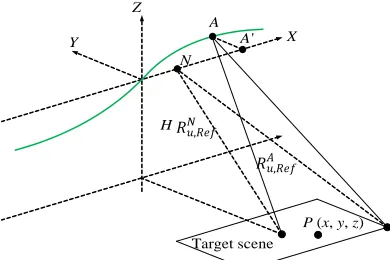
The geometry of the airborne or vehicle-based strip-map SAR is illustrated in Figure 1, in which the green solid curve indicates the real track of the radar, and the dotted line is the predicted ideal path. Strip-map SAR means that the illumination direction of the radar remains unchanged.
In the coordinate in Figure 1, the origin is at the center of the synthetic aperture. The forward velocity direction of the radar is along the X axis, and the Y-Z plane is the perpendicular plane of the nominal trajectory. The two points marked as N and A are respectively the nominal and actual locations of the radar platform at a certain azimuth-time, and the point marked as P is one arbitrary point scatter located at (x, y, z).
Assume that the pulse repeat interval (PRI) is Tr, then the slow time Tu is an integer multiple of Tr. Therefore, the ideal positions of the radar are evenly distributed along X-axis with an interval of V ·Tr, here V is the forward velocity.
X Y
Z
A
P (x, y, z) H
N A'
Target scene
The nominal and actual positions can be denoted as (V·Tu,0, H) and (V·Tu+Xu, Yu, H+Zu), here H is the altitude of the radar, and (Xu, Yu, Zu) is the motion error vector at slow-time Tu. Assuming that the entire synthetic aperture is Ls, then the nominal and actual distances between the radar and the point target are:
RNu =
(V ·Tu−x)2+y2+ (H−z)2 (1)
RAu =
(V ·Tu+Xu−x)2+ (Yu−y)2+ (H+Zu−z)2 (2)
LOS is the beam center of the radar antenna, and in Figure 1, it is vertical to FVD, whereas it may not be the common case. The motion error is usually divided into two components, which are the deviation along LOS and displacement along FVD. Here, the attitude variation is to be classified as error
in LOS. Hence in Figure 1, the motion errorN A = (Xu, Yu, Zu) can be divided into two parts, which
are errors in LOS and FVD respectively as the vectors AA= (0, Yu, Zu) andN A = (Xu,0,0), where A is the projection ofA onX axis. In the following analysis, they would be eliminated respectively in different methods.
If the transmitted signal is:
S(t, u) =p(t) (3)
Considering one single target, the reflected signal can be written as:
SN(t, u) = p
t−2·R N u c ·exp
−i·2π·
2·RuN λ
+fduN ·t
(4)
SA(t, u) = p
t−2·R A u c ·exp
−i·2π·
2·RAu λ
+fduA ·t
(5)
whereSN andSAare the nominal and actual data received by radar. tis the fast-time, uthe slow-time, λthe wavelength of the transmitted signal, andcthe speed of light. AndfduN/A= (2π/λ)·(dRN/Au /P RI), is the Doppler frequency at each slow-timeu, determined by the variation ofRN/Au within each PRI.
To compress the data, the matched filtering is applied usingp(t) as the reference signal. The phase term of fdu brings about a shift byfdu in the frequency domain and is calculated and compensated in advance. To compensate the Doppler shift, the signal is multiplied with the conjugate of the Doppler exponential term exp(−i·2πfduNt), and then the signal is correlated with the local generated reference in the range compression, and therefore the range compressed data can be written as:
˙
SN(t, u) = Pr
t−2·R N u c ·exp −i· 2π λ
·2·RNu
(6)
˙
SA(t, u) = Pr
t−2·R A u c ·exp −i· 2π λ
·2·RAu
(7)
Here, ˙S denotes the range compressed data andPr(τ) the cross-correlated function of the received and reference signal in the fast-time domain. In (6)–(7), although the Doppler shift is compensated, the phase corresponding to the target trajectory is still maintained, which is the data to be compressed in the azimuth dimension. Through the comparison between ˙SN and ˙SA, the errors act as the delay deviation Δτ and additional phase Δϕ, which are:
Δτ = 2· RuA−RNuc (8)
Δϕ =
2π
λ
·2· RAu −RNu (9)
3. BULK MOCO
3.1. Principle of the Bulk MOCO
and additional phase in the signal should be extracted so that the actual signal can match with the reference signal.
It can be observed in Figure 1 that (RA
u −RNu) is different for targets at different locations. Hence, different compensation filters should be applied to different targets, which is the fundamental concept of the bulk MOCO.
Since the bulk MOCO has been researched a lot in [18–26], here it is only simply mentioned for deriving the following residual error discussion.
The bulk MOCO is composed of two essential steps, firstof which is to compensate the bulk portion common to all the targets, and second is to deal with the residual portion. The schematic diagram is illustrated in Figure 2.
The target at the scene center is usually chosen as the reference target for the bulk MOCO. According to (8) and (9), the delay deviation and the additional phase of the reference target are:
ΔτRef = 2· RAu,Ref −RNu,Ref
c (10)
ΔϕRef = 2π
λ ·2· R A
u,Ref −RNu,Ref
(11)
For other targets, the residual phase error is the difference between Δϕand ΔϕRef:
ΔϕRes = Δϕ−ΔϕRef = 4π
λ · R
A u −RNu
− RAu,Ref−RNu,Ref (12)
And the residual delay deviation ΔτRes is proportional to ΔϕRes:
ΔτRes = ΔϕRes· λ 2π
c (13)
The residual error varies with the scene pixels, which affects the azimuth signals. Hence, it makes it inevitable to implement the residual MOCO during the azimuth compression but not in advance, so that the residual error should be added to the azimuth matched filter, and the final compressed data is undoubtedly to be impacted by the residual error.
3.2. Residual Error of the Bulk MOCO
To quantify the performance of the bulk MOCO, the component ρRes is introduced here as the
uncompensated factor or the residual factor.
ρRes =|ΔϕRes|max/|Δϕ| (14)
In the bulk MOCO, the motion error is the vector pointing from the nominal radar position to the real one, and therefore the motion error is composed of two factors, magnitude and orientations.
Raw Data
Range Compression
Image Shift by
Azimuth Compression
Shift by
Multiply by
Figure 2. Schematic diagram of the bulk MOCO.
X Y
Z
Scene
Nominal trajectory
0 20 40 60 80 100 Antenna Beam-width / degree
θ2=0°
r/R0=0.2
r/R0=0.4
r/R0=0.6
r/R0=0.8
0 20 40 60 80 100
An tenna Beam-width / degree θ2=30°
r/R 0=0.2
r/R 0=0.4
r/R 0=0.6
r/R0=0.8
0 20 40 60 80 100
Antenna Beam-width / degree
θ =60°2 r/R =0.2 0
r/R =0.4 0
r/R =0.6 0
r/R =0.8 0
0 0.2 0.4 0.6 0.8 1
Uncompensated factor
0 0.2 0.4 0.6 0.8 1
Uncompensated factor
0 0.2 0.4 0.6 0.8 1
Uncompensated factor
(a)
(b) (c)o o o
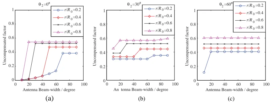
Figure 4. Maximum uncompensated factorρRes of the bulk MOCO.
Under certain orientation, ρ =|ΔϕRes|/|Δϕ| for different magnitudes is constant. While for the same magnitude, ρvaries with orientations and there exists the maximum value of ρ which isρRes in (14).
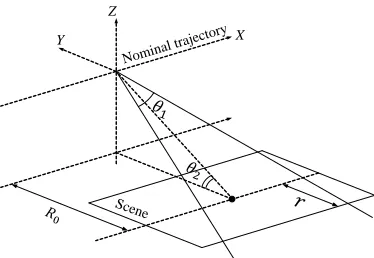
Obviously,ρRes is with relation to the position and the dimension of the target scene and the beam width of the radar antenna. All the above factors can be described by three parameters of (r/R0), θ1
and θ2 in Figure 3, herer is half the scene’s dimension along LOS,R0 is the range of the scene center,
θ1 is the beam width of the antenna andθ2 is the elevation angle.
Under the geometric model in Figure 3, ρRes of the bulk MOCO is calculated by statistic means whereρ for all orientations are calculated to obtain ρRes. The variation ofρRes with the change of the parameters is shown in Figure 4.
It can be seen from Figure 4 that when the dimension of the scene is comparable to the range of the scene center, the beam width antenna is larger than 60◦, and the elevation angle is larger than 30◦, the residual factorρRes is as large as around 0.6. In fact, for many practical cases, the range-dependent error is the dominant part, especially the error in FVD. Hence, a ‘resampling MOCO’ algorithm focusing on MOCO in FVD is proposed in Section 4 as an auxiliary of bulk MOCO.
4. RESAMPLING MOCO
4.1. Principle of the Resampling MOCO
As discussed in previous sections, the LOS error is instantaneous, while the FVD error is different and is accumulation of the forward velocity variation. Hence, during long data acquisition time, the FVD error may reach a huge value. The basic concept of the resampling MOCO is to limit the FVD error within one azimuth sample via data restructuring.
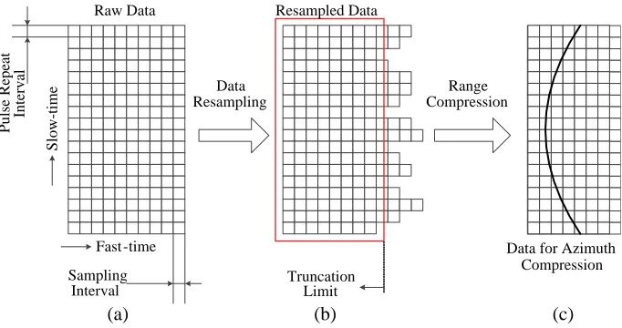
Generally, since PRI (Tr) and sampling frequency in range (FS) are both fixed, the received data can be divided into several range bins corresponding to each slow-time, and the amount of data of each range bin is Tr·FS. As shown in Figure 5(a), for an ideal case, the number of samples in each range bin should be always identical, and the distance between adjacent samples in the azimuth dimension should be the product ofTr and the forward velocity Vu, that is:
Lu =Tr·Vu (15)
IfVuvaries with slow-timeu, thenLufluctuates so that azimuth sampling turns to be non-uniform. In this case, in order to obtain constantLu, the tuneable PRI should be:
˜ Tr = ¯L
Vu (16)
Here, ¯L is the average interval of azimuth samples, and the current number of samples ˜Tr·FS is not identical any more for different range bins, as shown in Figure 5(b).
Data Resampling
Range Compression
Data for Azimuth Compression Raw Data
Fast-time
Resampled Data
Slow-time
Sampling Interval
Pulse Repeat
Interval
Truncation Limit
(a) (b) (c)
Figure 5. Schematic diagram of the resampling MOCO.
azimuth bins, as illustrated by the large red frame in Figure 5(b). Finally, the range compressed data will be processed in azimuth dimension by conventional image formation algorithm.
From Figure 5, the concept of resampling MOCO is the tunable sampling according to the forward velocity variation which avoids error accumulation in FVD, but this process shortens the range bin at the same time.
Essentially, although the raw data are resampled and truncated, each range sample still represents the same length in the range dimension, and the only change is the length of the range bin. In other words, the duration of the range signal is shortened. However, if we consider the PRI equals 1 ms, then the distance corresponding to each range bin is the product of PRI and the speed of light and equals 300 km, which is enough for most of the airborne and vehicle-based SAR systems even truncated by 20%.
4.2. Residual Error of the Resampling MOCO
In the proposed algorithm, the original idea to resample the raw data is to rearrange the azimuth samples to be uniform. However, since the velocity of radar can be different in each PRI, it should be noticed that for each certain fast-time, there is still slight deviation in the azimuth samples. And this residual error can be written as (see Appendix A):
ERes =
1− Vmin Vmax
·Tr·Vave (17)
Here, Vmin, Vmax and Vave are respectively the minimum, maximum and average velocities of the radar.
Even in the most extreme case that we can assume, the speed of the radar is in the range of 500±25 m/s. If PRF is 2 kHz, the residual FVD displacement should be around 2 cm according to (17). Based on Figure 2 and Figure 4, even the beam width is as large as 60◦, the path error of the signal, by converting from the residual displacement in FVD, is 1 cm. Then the path error of the round trip is 2 cm, and the sequent phase error is acceptable to most of SAR systems.
Furthermore, according to (17), we can also reduce the residual error by increasing the PRF. Hence, from another point of view, if we set, in advance, a threshold for the residual error, then PRF can be calculated as:
PRF = 1/Tr =
1− Vmin Vmax
·Vave/ERes (18)
5. MOCO WITH BACK-PROJECTION ALGORITHM
In this section, the proposed MOCO method is to be applied during the image formation and specifically the back-projection algorithm (BPA) is involved.
5.1. Fundamental and Modified Back-projection Algorithms
Figure 6 shows the fundamental SAR image formation process. Firstly, the range compressed data is obtained by applying the matched filtering in advance. The matched filtering process is specifically the correlation between the received signal and transmitted signal. Then the scene image can be obtained
Received Signal
Back -projection Reference
Signal
Image Range
compression
Figure 6. Fundamental BPA block diagram.
Range
Compressed
Data
Data @ Slow-time u 1
Data @ Slow-time u2
Data @ Slow-time u M
Targets Range @ Slow-time
u1
Targets Range @ Slow-time
u2
Targets Range @ Slow-time
uM
Image Targets distribution @ Slow-time u1
Targets distribution @ Slow-time u2
Targets distribution @ Slow-time uM
Figure 7. Back projection processing.
Received Signal
Back-projection
Reference Signal
Image Resampling &
truncating MOCO
Resampling & truncating
MOCO
Residual MOCO Range
compression
Bulk MOCO
Received Signal
Back-projection
Reference Signal
Image Resampling &
truncating MOCO Bulk
MOCO
Resampling & truncating
MOCO
Residual MOCO Range
compression
(a)
(b)
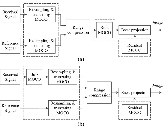
after back projection process. Detailed back-projection processing is presented in Figure 7 which includes several steps. First step is the projection calculation implemented for all slow-time fromu1 to uM. For each slow-time u, the target scene is meshed into several grids, and for each grid, the round trip range is calculated. The range compressed data are allocated to all grids according to the calculated range. The final step of the back-projection algorithm is the integration throughout the illuminating duration. Based on the fundamental BPA block diagram, the MOCO procedure is added in Figure 8.
Firstly, to eliminate the FVD deviation, resampling MOCO is applied to the raw data before the range compression. Secondly, to remove LOS error, bulk MOCO is applied to compensate the corresponding delay shift and additional phase. The range compression is a linear process for the phase, so the bulk MOCO can either be carried out before the range compression or after that, as can be seen from Figures 8(a) and (b). Last, as a remaining step of the bulk MOCO, the residual MOCO is applied during the back projection process.
5.2. Simulation Results
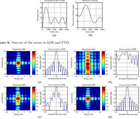
The feasibility of bulk MOCO has been verified in a few applications, while the resampling MOCO method is to be firstly tested here. Therefore, for a general vehicle-based SAR case, a typical set of error in LOS is given as the simulation parameter setting, but the error in FVD is given as magnified to verify
0 1000 2000 3000 4000
0 5 10 15 20 25 Time [ms] Deviatin [cm]
Deviation in line of sight
0 1000 2000 3000 4000
0 5 10 15 20 Time [ms]
Receivers Velocity [mps]
Receivers Velocity
(a) (b)
Figure 9. One set of the errors in LOS and FVD.
Range [m]
Azimuth [m]
Magnitude [dB]
-10 -5 0 5 10 -35
-30 -25 -20 -15 -10 -5 0
-10 0 10
Azimuth Direction [m]
Magnitude [dB]
Cross-section of PSF
Range [m]
Azimuth [m]
Magnitude [dB]
-10 -5 0 5 10 -35
-30 -25 -20 -15 -10 -5 0 0 10
Azimuth Direction [m]
Magnitude [dB]
Cross-section of PSF
Range [m]
Azimuth [m]
Magnitude [dB]
-10 -5 0 5 10 -35
-30 -25 -20 -15 -10 -5 0
-10 0 10
Azimuth Direction [m]
Magnitude [dB]
Cross-section of PSF
Range [m]
Azimuth [m]
Magnitude [dB]
-10 -5 0 5 10 -35
-30 -25 -20 -15 -10 -5 0
-10 0 10
Azimuth Direction [m]
Magnitude [dB]
Cross-section of PSF -10 -5 0 5 10 -30 -25 -20 -15 -10 -5 0 -10 -5 0 5 10 -10 -30 -25 -20 -15 -10 -5 0 -10 -5 0 5 10 -10 -5 0 5 10 -30 -25 -20 -15 -10 -5 0 -30 -25 -20 -15 -10 -5 0 (a) (b) (c) (d)
the performance of the proposed method, as shown in Figure 9. The simulated point spread functions (PSFs) and the azimuth cross-sections are shown in Figure 10 to compare the focusing performance.
According to Figure 10, firstly, the imaging without any motion error is processed for comparison (Figure 10(a)) which has a common azimuth side-lobe as−13.2 dB, followed by the PSF in Figure 10(b) considering the motion error in Figure 9 but without any MOCO, and therefore the azimuth compression is failed, since the compressed pulse is not peaking at the assumed delay and moreover the pulse shape no longer a Sinc(·) function. In Figure 10(c), the motion error is compensated by bulk MOCO only, and the Sinc(·) shape is recovered but with a higher side-lobe ratio as −7 dB which is high for radar remote sensing applications. At last in Figure 10(d), the motion error is compensated by integrated bulk MOCO and resampling MOCO. From the PSF, the azimuth signal is compressed correctly. From the range cross-section, the SLR is−13.3 dB, in the same level as the ideal case Figure 10(a). According to the simulation results, the proposed algorithm performs much better than the original bulk MOCO, and the origin PSF has been almost recovered.
6. DISCUSSION
Generally speaking, the phase and envelope errors caused by the motion deviation are constituted by both linear and non-linear terms. The motion error is totally random, while the image formation algorithm is processed as pulse compression based on the relevance of the signals. In this paper, the effect of the error to both the compression procedure and compressed data is concerned.
The essence of the MOCO may be regarded as the pre-processing of raw data, and under arbitrary SAR topologies, the proposed resampling MOCO method can be always employed as an auxiliary to other commonly used MOCO methods, bringing about improved MOCO performances. The phase error can always be compensated through multiplying with the signal carrying a phase opposite to the phase error, while the solution for the envelope advance or delay is always signal shift in the envelope, and resampling can be utilized for stretching the envelope. In this paper, the motion error is divided into two types, which are errors in LOS and FVD, respectively. The motion methods selected for the LOS deviation is the widely used bulk MOCO, while for FVD displacement, a novel ‘resampling & truncation’ MOCO algorithm is proposed.
For the bulk MOCO algorithm, the residual error, or the uncompensated factor is firstly statistically
analyzed. And for the proposed ‘resampling’ MOCO, the residual error is analyzed as well. The
feasibility of the proposed algorithm is verified by the simulation results, but it is still to be proved in the practical applications.
Till now, all the analysis and simulations in this paper mainly focus on the mono-static SAR. While for bi-static case, the motion errors of both the transmitter and receiver need to be taken into account, which is more complicated than the mono-static topologies. On one hand, if one of the transmitters or receivers is stationary or moves in a constant speed, the proposed algorithm can be applied directly. On the other hand, if the transmitter and receiver have different FVD deviations, modified algorithms should be concerned to satisfy different resampling requirements.
APPENDIX A. RESIDUAL ERROR OF RESAMPLING MOCO
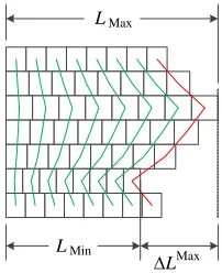
A description about the range of the residual error of resampling MOCO has been given in Figure A1. Grids of each row represent the range-sampled data in the corresponding slow-time, and the width of every grid indicates the distance that the radar has travelled in the interval of one range sample Ts which is the reciprocal of the sampling frequency Fs. In Figure A1, there is the same number of grids in each line, which means that samples of each range bin have been truncated into same length.
Since the grids in the same column belong to one azimuth bin, the grids of each azimuth bin are connected by the solid line. It can be seen very clearly that the rightmost azimuth bin in Figure A1 has the maximum fluctuation, so the column connected by the red solid line will be considered to analyze the residual error of resampling MOCO.
Since the whole length of each line denotes the radar trajectory in this range bin, the maximum length should be the origin distance between adjacent azimuth samples:
LMax
LMin
ΔLMax
Figure A1. Raw data after resampling and truncation.
Here,Vave is the average speed of the radar platform, and the number of samples of each range bin should be:
N = Lmax FS·Vmax
= Tr·Vave FS·Vmax
(A2)
Hence, the minimum length in the azimuth dimension of all the range bins should be:
Lmin=N·FS·Vmin = Tr·Vave·Vmin
Vmax
(A3)
Then the maximum difference of the samples in each azimuth bin should be:
ΔLmax=Lmax−Lmin =Tr·Vr¯ ·
1− Vmin Vmax
(A4)
Here, ΔLmax is the maximum residual displacement in FVD after data resampling.
REFERENCES
1. Cumming, I. G., et al., Digital Signal Processing of Synthetic Aperture Radar Data: Algorithms and Implementation, Artech House, Norwood, 2004.
2. Fornaro, G., G. Franceschetti, and S. Perna, “Motion compensation errors: Effects on the accuracy of airborne SAR images,”IEEE Transactions on Aerospace and Electronic Systems, Vol. 41, No. 4, 1338–1352, 2005.
3. Kirk, Jr., J. C., “Motion compensation for synthetic aperture radar,” IEEE Transactions on
Aerospace and Electronic Systems, Vol. 3, 338–348, 1975.
4. Franceschetti, G., et al., “SAR sensor trajectory deviations: Fourier domain formulation and extended scene simulation of raw signal,”IEEE Transactions on Geoscience and Remote Sensing, Vol. 44, No. 9, 2323–2334, 2006.
5. Buckreuss, S., “Motion errors in an airborne synthetic aperture radar system,” European
Transactions on Telecommunications, Vol. 2, No. 6, 655–664, 1991.
6. Wu, H. and T. Zwick, “Micro-air-vehicle-borne near-range SAR with motion compensation,”
Progress In Electromagnetics Research, Vol. 145, 11–18, 2014.
7. Wu, H. and T. Zwick, “Octave division motion compensation algorithm for near-range wide-beam SAR applications,” Progress In Electromagnetics Research, Vol. 144, 115–122, 2014.
8. Long, T., et al., “A DBS Doppler centroid estimation algorithm based on entropy minimization,”
IEEE Transactions on Geoscience and Remote Sensing, Vol. 49, No. 10, 3703–3712, 2011.
9. Zhao, Y., et al., “A method of Doppler frequency rate estimation for millimeter-wave missile-borne
SAR,”2012 IEEE 5th Global Symposium on Millimeter Waves (GSMM), 604–607, 2012.
11. Wei, S.-J. and X.-L. Zhang, “Sparse autofocus recovery for under-sampled linear array SAR 3-D imaging,”Progress In Electromagnetics Research, Vol. 140, 43–62, 2013.
12. Moreira, J. R., “A new method of aircraft motion error extraction from radar raw data for real time motion,”IEEE Transactions on Geoscience and Remote Sensing, Vol. 28, No. 4, 620, 1990.
13. Zhang, L., et al., “A robust motion compensation approach for UAV SAR imagery,” IEEE
Transactions on Geoscience and Remote Sensing, Vol. 50, No. 8, 3202–3218, 2012.
14. De Macedo, K. A. C., R. Scheiber, and A. Moreira, “An autofocus approach for residual motion
errors with application to airborne repeat-pass SAR interferometry,” IEEE Transactions on
Geoscience and Remote Sensing, Vol. 46, No. 10, 3151–3162, 2008.
15. Xing, M., et al., “Motion compensation for UAV SAR based on raw radar data,”IEEE Transactions on Geoscience and Remote Sensing, Vol. 47, No. 8, 2870–2883, 2009.
16. Wahl, D., et al., “Phase gradient autofocus-a robust tool for high resolution SAR phase correction,”
IEEE Transactions on Aerospace and Electronic Systems, Vol. 30, No. 3, 827–835, 1994.
17. Isernia, T., et al., “Synthetic aperture radar imaging from phase-corrupted data,”IEE Proceedings — Radar, Sonar and Navigation, Vol. 143, No. 4, 268–274, 1996.
18. Liu, B. and W. Chang, “Range alignment and motion compensation for missile-borne frequency stepped chirp radar,”Progress In Electromagnetics Research, Vol. 136, 523–542, 2013.
19. Moreira, A. and Y. Huang, “Airborne SAR processing of highly squinted data using a chirp scaling
approach with integrated motion compensation,” IEEE Transactions on Geoscience and Remote
Sensing, Vol. 32, No. 5, 1029–1040, 1994.
20. Rodriguez-Cassola, M., et al., “Efficient time-domain image formation with precise topography
accommodation for general bistatic SAR configurations,” IEEE Transactions on Aerospace and
Electronic Systems, Vol. 47, No. 4, 2949–2966, 2011.
21. Prats, P., et al., “Comparison of topography- and aperture-dependent motion compensation algorithms for airborne SAR,”IEEE Geoscience and Remote Sensing Letters, Vol. 4, No. 3, 349– 353, 2007.
22. Zamparelli, V., S. Perna, and G. Fornaro, “An improved topography and aperture dependent
motion compensation algorithm,” 2012 IEEE International Geoscience and Remote Sensing
Symposium (IGARSS), 5805–5808, 2012.
23. De Macedo, K. A. C. and R. Scheiber, “Precise topography- and aperture-dependent motion compensation for airborne SAR,” IEEE Geoscience and Remote Sensing Letters, Vol. 2, No. 2, 172–176, 2005.
24. Sun, G., et al., “Focus improvement of highly squinted data based on azimuth nonlinear scaling,”
IEEE Transactions on Geoscience and Remote Sensing, Vol. 49, No. 6, 2308–2322, 2011.
25. Tian, B., D.-Y. Zhu, and Z.-D. Zhu, “A novel moving target detection approach for dual-channel SAR system,” Progress In Electromagnetics Research, Vol. 115, 191–206, 2011.
26. Zhu, D., Y. Li, and Z. Zhu, “A keystone transform without interpolation for SAR ground moving-target imaging,” IEEE Geoscience and Remote Sensing Letters, Vol. 4, No. 1, 18–22, 2007.
27. Franceschitti, G. and R. Lanari, Synthetic Aperture Radar Processing, CRC Press, 1999.
28. Fornaro, G., “Trajectory deviations in airborne SAR: Analysis and compensation,” IEEE
Transactions on Aerospace and Electronic Systems, Vol. 35, No. 3, 997–1009, 1999.