Novel Finite Airy Array Beams Generated from Gaussian Array
Beams Illuminating an Optical Airy Transform System
Lahcen Ez-Zariy, Zoubir Hricha, and Abdelmajid Belafhal*
Abstract—In this work, a novel family of Finite Airy array beams have been produced by an optical Airy transform system illuminated by Gaussian Array beams. Based on the generalized Huygens-Fresnel integral, an analytical expression is developed to describe the pattern properties of the beam generated at the output plan of the optical system. The well-known Finite Airy beam generated from the fundamental Gaussian beam using an optical Airy transform system is deduced, here, as a particular case of the main result of the actual study. Numerical calculations are performed to show the possibility to create a multitude of Finite Airy array beams with controllable parameters depending on the number of beamlets, the distance between the adjacent modules and the positions and orientations of the beamlets.
1. INTRODUCTION
In recent years, Airy beams have attracted great interest due to their unique features, including non-spreading, self-healing, self-acceleration (even in the absence of external force) and parabolic trajectories [1–5]. These characteristics lead them to be good candidate in many applications such as optical micro-manipulation [6], curved plasma channel generation [7, 8], optical microscopy and scanning microscopy using optical Airy bullets [9], vacuum electron acceleration [10], trapping and guiding micro-particles [11, 12]. Several methods have been devoted to generate the Airy beams with finite energy. Among these, we can cite the cubic phase, 3/2 phase only pattern and three-wave mixing processes in asymmetric nonlinear photonic crystals [13–18].
The integral transformations including Fourier, Hilbert and Airy transforms have long been of interest due to their wide applications in solving many problems in applied mathematics, engineering sciences and optics. The Airy transform which was firstly introduced in mathematics by Widder in 1979 [19] has been used in physics to solve the Schr¨odinger equation for free particle and free fall [20]. In optics, the concept of Airy transform has been applied in solving the free-space wave equation of light beams [21]. Recently, Jiang et al. [22] have implanted the Airy transform technique as a novel tool to generate and control the Finite Airy beams. The authors have also derived the amplitude expression of the so-called Airy-related beam by using an optical Airy transform system illuminated by a flattened Gaussian beam [23].
On the other hand, increasing attention has been paid to laser Array beams over the last few decades due to their applications in high-power laser systems, inertial confinement fusion and high-energy weapons and free-space optical communications [24, 25]. Particularly, the Gaussian Array beams, which are constructed by combining multiple separate beamlets, have been the subject of several studies [26– 32].
Received 19 April 2016, Accepted 5 July 2016, Scheduled 13 July 2016
* Corresponding author: Abdelmajid Belafhal ([email protected]).
In this work, by means of the two-dimensional optical Airy transform technique and with a setup including additional lens before a spatial light modulator [22], we introduce an analytical expression of a new Finite Airy Array beams family generated by an optical Airy transform system illuminated by Gaussian Array beams. Compared to a single conventional Airy beam, the creation of Airy Array beam can enable the parallel processing with intrinsic high processing efficiency for various applications; i.e., nanofabrication, generation of curve plasmon channel, light sheet microscopy, etc. Besides, compared to the Airy beam generated by Fourier transform of Gaussian beam modulated by a cubic phase [4], the Airy transform setup used in this work presents some practical advantages in controlling the output beam [22, 23]. It is provided that when the incident Gaussian beam is translated by a vector in the input plane, the output Airy beam will be translated by the same vector in the output plane. The optical Airy transform setup permits the control of the launch angle by varying the axial position of the beam waist. Furthermore, it is useful in directly producing and controlling new Airy beams from initial finite energy Airy beams [22]. In this paper, the properties of the new Airy Array beams generated are analyzed and discussed numerically. The obtained results are consistent with the previous works which can be regarded as particular cases of this study.
The paper is structured as follows. In the coming section, we present the distributions of the two-dimensional Gaussian Array beams as incident beams and their transverse intensity patterns at the source plan are illustrated. In Section 3, The mathematical model describing the propagation of a laser beam through an optical Airy transform system is presented, and an analytical expression of a Finite Airy Array beam generated from the Gaussian Array beam illuminating the optical Airy transform system is derived. The previous result concerning the generation of the Finite Airy beam from the fundamental Gaussian beam is deduced as a particular case of our main study. Some numerical calculations are carried out in Section 4 to illustrate the effects of the initial beam and the optical system parameters on the properties of generated beam. In the last section, we summarize the main results of our study.
2. GAUSSIAN ARRAY BEAM
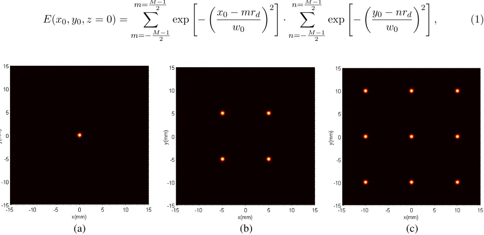
At the source plane (z = 0), consider a Gaussian array beam composed of M ×M beamlets. In the Cartesian coordinate system, the cross spectral density of the resulting beam is expressed as [26]
E(x0, y0, z= 0) =
m=M2−1
m=−M2−1
exp
−
x0−mrd w0
2
·
n=M2−1
n=−M2−1
exp
−
y0−nrd w0
2
, (1)
(a) (b) (c)
wherew0 is the waist width of each Gaussian beamlet amplitude distribution,rdthe separation distance between adjacent modules and M the number of beamlets. Fig. 1 depicts the transverse intensity distribution of the Gaussian beam array at source plane at z = 0 for different M ×M. From the
(c)
(a) (b)
(d)
Figure 2. Intensity distribution contours of the Gaussian beam Arrays for different values of rd: (a) rd= 0, (b) rd= 5 mm, (c) rd= 10 mm and (d) rd= 20 mm, withM = 2 andw0 = 0.5 mm.
(a) (b) (c)
plots of this figure, it is shown that whatever the value of M, each set of M Gaussian Array beams presentsM×M adjacent modules of Gaussian patterns. The parameters chosen in the simulations are w0= 1 mm, and the beamlets are separated by rd= 10 mm.
Figure 2 illustrates the intensity contours for the Gaussian beam arrayM×M withM = 3 and for various rd. It is clear that the distance between adjacent modules increases when rd increases. Fig. 3 is as Figs. 1 and 2, but with a fixed M×M,rd respectively and for various w0. The graphics of this
figure show that the beamlets keep their numbers and their separated distances and become very large when w0 increases.
3. GENERATION OF FINITE AIRY ARRAY BEAM BY AN OPTICAL AIRY TRANSFORM SYSTEM
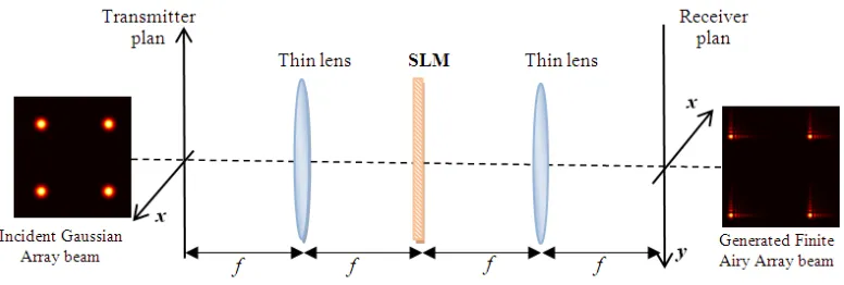
Consider an optical Airy transform system as schematized in Fig. 4. The optical system is composed of two thin lenses of focal length f and a spatial light modulator (SLM) used to convert the phase of the light heating its center by imposing on it a phase modulationφ.
Figure 4. Schematic representation of the conversion of a Gaussian Array beam to a Finite Airy Array beam by means of the optical Airy transform system.
Assume that the transverse electrical field distribution of the incident beam is E0(x0, y0). So, the
electrical field E1(x1, y1) of the beam received at an arbitrary point of the transverse SLM plane (just
before the SLM) is given fromE0(x0, y0) using the generalized Huygens-Fresnel integral [33] as
E1(x1, y1) =
2π
ikfexp(ikf)
+∞
−∞
+∞
−∞
E0(x0, y0) exp
−ik
f (x0x1+y0y1)
dx0dy0, (2)
wheref is the focal length of the lens (see Fig. 4).
The phase pattern of the SLM is considered to be [20]
φ(x1, y1) =
α3k3x+β3ky3
3 −(4kf +π), (3)
whereα,β are real constants, andk is the wave number,kx =kx1/f and ky =ky1/f.
Thus, the electrical field of the beam just behind the SLM is
E2(x1, y1) =E1(x1, y1) exp(iφ(x1, y1)) (4)
Finally, always based on the generalized Huygens-Fresnel diffraction principle [33], the outgoing electrical field of the beam exiting the output plane of the Airy transform system is written as
E(x, y) = 2π
ikf exp(ikf)
+∞
−∞
+∞
−∞
E2(x1, y1) exp
−ik
f (xx1+yy1)
Inserting Eq. (4) into (5) and by taking account of Eqs. (2) and (3), the electric field at the output plane of the optical Airy transform system could be obtained directly from E0(x0, y0) by means of the
mathematical Airy transform model which is expressed by two-dimensional double integral as [20]
E(x, y) = 1
|αβ| +∞ −∞ +∞ −∞
E0(x0, y0)Ai
x−x0
α
Ai
y−y0
β
dx0dy0, (6)
whereAi(·) is the Airy function.
Suppose that the optical Airy transform system is illuminated by a Gaussian Array beam whose electric field is given by Eq. (1). The electrical field of the created beam at the outgoing plane of the Airy optical system is obtained by the introduction of Eq. (1) into Eq. (3). This electric field reads as
E(x, y) = A0
|αβ|
m=M2−1
m=−M2−1
exp
−m2rd2 w20
Em(x)·
n=M2−1
n=−M2−1
exp
−n2rd2 w20
·En(y), (7a)
where
Em(x) =
+∞
−∞
Ai
x−x0
α
exp
− 1
w20
x20+
2mrd w02
x0
dx0, (7b)
and
En(y) =
+∞
−∞
Ai
y−y0
β
exp
− 1
w20
y02+
2nrd w20
y0
dy0. (7c)
The calculation of the electrical field at receiver plane of the optical Airy transform system will halt on solving the integrals Em(x) and En(y) which are similar and could be calculated by the same way. So, in this case, we developEm(x) and derive from it En(y).
Then, for this reason, we recall the representation of Airy function into an infinite integral which is written by [20]
Ai(s) = 1 2π +∞ −∞ exp iu 3
3 +ius
du, (8)
according to this expression, we obtain
Ai
x−x0
α = 1 2π +∞ −∞ exp iu 3 3 + iux α − iu αx0
du. (9)
Substituting this last integral in the above expression of Eq. (7b),Em(x) becomes
Em(x) = 1 2π +∞ −∞ exp iu 3 3 + ix αu ⎧⎨ ⎩ +∞ −∞ exp − 1 w2 0
x20+
2mrd w2 0 −iu α x0 dx0 ⎫ ⎬
⎭du. (10)
By the recall of the well-known integral of Ref. [34]
+∞
−∞
exp−p2y2±qydy =
√
π p exp
q2 4p2
, (11)
with Re(p2) > 0, the x-electrical field component of the beam generated at the receiver plan of the
optical Airy transform yields to
Em(x) = w
0√π
2π exp
m2r2d w20
+∞ −∞ exp iu 3
3 +i
iw20
4α2
u2+i
and by applying the following well-known integral [20], +∞ −∞ exp iu 3
3 +iau
2+ibu
du= 2πexp
ia
2a2 3 −b
Aib−a2. (13)
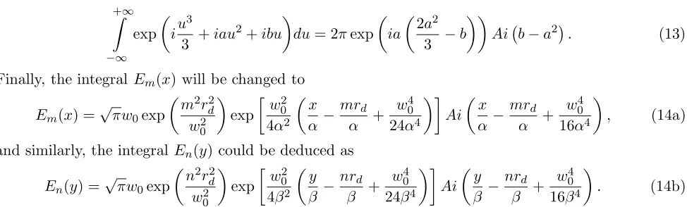
Finally, the integral Em(x) will be changed to
Em(x) =
√
πw0exp
m2r2d w2
0
exp
w02
4α2
x
α −
mrd
α +
w04
24α4
Ai x α − mrd α +
w40
16α4
, (14a)
and similarly, the integral En(y) could be deduced as
En(y) =
√
πw0exp
n2r2d w02
exp
w2 0
4β2
y β − nrd β + w4 0
24β4
Ai y β − nrd β + w4 0
16β4
. (14b)
By replacing the expressions ofEm(x) andEn(y) into Eq. (7a), the final expression of the electric field E(x, y) of the Gaussian beam array propagating through an optical Airy transform in the output plane of this system is given by
E(x, y) = A0πw
2 0
|αβ|
m=M2−1
m=−M2−1
exp
w20
4α2
x
α −
mrd
α +
w40
24α4
Ai x α − mrd α +
w40
16α4
×
n=M2−1
n=−M2−1
exp
w20
4β2
y
β −
nrd
β +
w40
24β4
Ai y β − nrd β +
w40
16β4
. (15)
Equation (15) expresses the electrical field distribution of a novel Finite Airy Array beam produced at an arbitrary point of the output plan of an optical Airy transform system illuminated by an Array Gaussian beam. It is worthy to note that this novel generated beam can be controlled numerically, by means of the different parameters corresponding to the incident beam and the optical Airy transform system.
When the number of beamletsM is equal to 1 (M = 1), the incident Gaussian beam array changes to a fundamental Gaussian beam expressed by
E(x0, y0, z= 0) =A0exp
−x20+y20
w0
2
. (16)
Under the same condition, the expression of the beam generated at the receiver plane of optical Airy transform system reduces to
E(x, y) =A0πw
2 0
|αβ| exp
w20
4α2
x α+
w40
24α4
Ai
x α+
w40
16α4
×exp
w20
4β2
y β+
w40
24β4
Ai
y β +
w04
16β4
. (17)
This formula is similar to Eq. (11) of Ref. [22] corresponding to the generation of the Finite Airy beam from the fundamental Gaussian beam using the Airy transform system. So, our finding generalizes the result of Ref. [22].
It is worthy to note that the self-healing property of the Airy array beams, considered the common characteristics for the nondiffracting beams, can be demonstrated theoretically from considering the self-healing character of each conventional single Airy beam which is contained in the Array beam.
4. NUMERICAL SIMULATIONS
In this section, based on the main expression established in Eq. (15), some numerical calculations are performed in order to study the effects of some parameters on the properties patterns of the beam generated at the receiver plan of the optical system.
(a) (b) (c)
Figure 5. Transverse intensity distributions of the generated Finite Airy Array beams for different values ofM: (a)M = 1, (b) M = 2, and (c) M = 3, with rd= 40 mm, w0= 0.5 mm and α=β =−1.
(a) (b) (c)
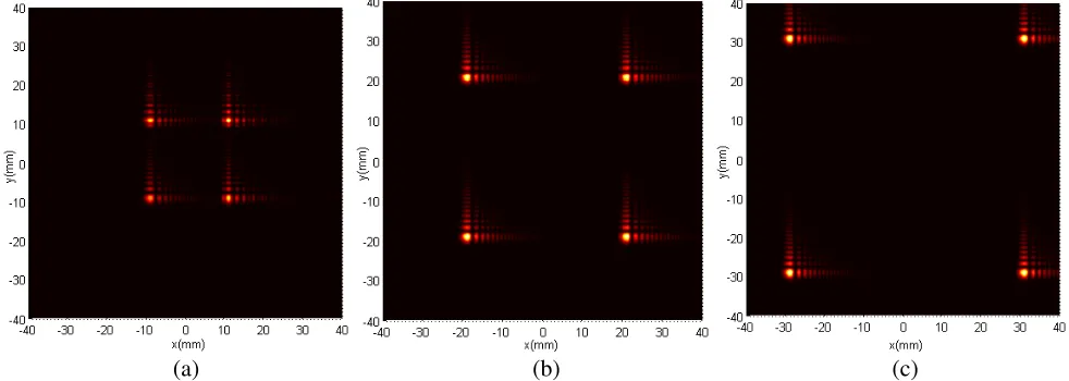
Figure 6. Transverse intensity distributions of the generated Finite Airy beams Arrays for different values ofrd: (a) rd= 20 mm, (b)rd= 40 mm and (c)rd= 60 mm, with M = 2 and w0= 0.5 mm.
parametersM×M, withrd= 40 mm,w0 = 0.5 mm andα=β =−1. As can be seen from the drawings,
we can control the number of beamlets in the produced Finite Airy array beam by convenient choice of numberM of the beamlets contained in the input Gaussian array beam. Especially, the single Airy beam is obtained when a single Gaussian is involved.
Moreover, in Fig. 6, we display the transverse intensity of the generated Finite Airy Array beams for different separation distances between the adjacent modules, (a) rd= 20 mm, (b) rd = 40 mm and (c) rd= 60 mm, with M = 2 and w0 = 0.5 mm. From the plots of this figure, it is noticeable that as
the separation distance between the adjacent modules of the incident beam increases, the separation distance between adjacent modules increases too.
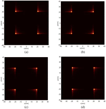
The plots in Fig. 7 show the possibility of inversing the orientations of the obtained Airy array beams by changing the signs of the optical Airy parametersαandβ. This effect is due to the change of localization of the single Airy modes contained in the Array beam from the third to the fourth quadrant for example when α and β change from positive to negative values as demonstrated in [22].
(c)
(a) (b)
(d)
Figure 7. Transverse intensity distributions of the generated Finite Airy Array beams for different values ofα andβ: (a) α=β =−1; (b)α =−β=−1; (c)α=β = 1 and (d)α=−β= 1, withM = 2, rd= 40 mm and w0= 0.5 mm.
5. CONCLUSION
Based on the generalized Huygens-Fresnel integral, a closed form expression of a novel Finite Airy array beam generated from the Gaussian array beam through an optical Airy transform system is developed. The investigation about the generation of the Finite Airy beam from the fundamental Gaussian beam, using an optical Airy transform system, is deduced as a particular case of our principal result. The numerical calculations show that the Airy optical system can be used as a tool to convert the Gaussian array beam into a Finite Airy Array beam with controllable parameters: number of beamlets, distance between the adjacent modules, positions and orientations of the modules of the Airy array beams produced by the optical Airy transform system. The findings of this research may be used in several practical applications such as manipulating, transport, guiding and trapping of particles.
REFERENCES
1. Berry, M. V. and N. L. Balazs, “Non-spreading wave packet,”Am. J. Phys., Vol. 47, 264–267, 1979. 2. Broky, J., G. A. Siviloglou, A. Dogariu, and D. N. Christodoulides, “Self-healing properties of
optical Airy beams,”Optics Express, Vol. 16, No. 20, 12880–12891, 2008.
4. Siviloglou, G. A., J. Broky, A. Dogariu, and D. N. Christodoulides, “Ballistic dynamics of Airy beams,”Optics Letters, Vol. 33, No. 3, 207–209, 2008.
5. Siviloglou, G. A. and D. N. Christodoulides, “Accelerating finite energy Airy beams,” Optics Letters, Vol. 32, 979–981, 2007.
6. Baumgartl, J., M. Mazilu, and K. Dholakia, “Optically mediated particle clearing using Airy wavepackets,” Nature Photonics, Vol. 2, No. 13, 675–678, 2008.
7. Polynkin, P., M. Kolesik, J. V. Moloney, G. A. Siviloglou, and D. N. Christodoulides, “Curved plasma channel generation using ultraintense Airy beams,” Science, Vol. 324, No. 5924, 229–232, 2009.
8. Polynkin, P., M. Kolesik, and J. Moloney, “Filamentation of femtosecond laser Airy beams in water,” Physical Review Letters, Vol. 103, No. 14, 123902, 2009.
9. Chong, A., W. H. Renninger, D. N. Christodoulides, and F. W. Wise, “Airy-Bessel wave packets as versatile linear light bullets,”Nature Photonics, Vol. 4, No. 2, 103–106, 2010.
10. Li, J. X., W. P. Zang, and J. G. Tian, “Vacuum laser-driven acceleration by Airy beams,” Optics Express, Vol. 18, No. 7, 7300–7306, 2010.
11. Zheng, Z., B. Zhang, H. Chen, J. Ding, and H. Wang, “Optical trapping with focused Airy beams,” Applied Optics, Vol. 50, No. 1, 43–49, 2011.
12. Zhang, P., J. Prakash, Z. Zhang, M. S. Mills, N. K. Efremidis, D. N. Christodoulides, and Z. Chen, “Trapping and guiding microparticles with morphing autofocusing Airy beams,” Optics Letters, Vol. 36, No. 18, 2883–2885, 2011.
13. Dai, H. T., X. W. Sun, D. Luo, and Y. J. Liu, “Airy beams generated by binary phase element made of polymer dispersed liquid crystals,” Optics Express, Vol. 17, 19365–19370, 2009.
14. Hu, Y., P. Zhang, C. Lou, S. Huang, J. Xu, and Z. Chen, “Optimal control of the ballistic motion of Airy beams,”Optics Letters, Vol. 35, No. 15, 2260–2262, 2010.
15. Polynkin, P., M. Kolesik, J. Moloney, G. Siviloglou, and D. N. Christodoulides, “Extreme nonlinear optics with ultra-intense self-bending Airy beams,” Optics and Photonics News, Vol. 21, No. 11, 38–43, 2010.
16. Cottrell, D. M., J. A. Davis, and T. M. Hazard, “Direct generation of accelerating Airy beams using a 3/2 phase-only pattern,” Optics Letters, Vol. 34, No. 20, 2634–2636, 2009.
17. Ellenbogen, T., N. Voloch-Bloch, A. Ganany-Padowicz, and A. Arie, “Nonlinear generation and manipulation of Airy beams,”Nature Photonics, Vol. 3, No. 7, 395–398, 2009.
18. Dolev, I., T. Ellenbogen, N. Voloch-Bloch, and A. Arie, “Control of free space propagation of Airy beams generated by quadratic nonlinear photonic crystals,” Applied Physics Letters, Vol. 95, No. 20, 201112-201112, 2009.
19. Widder, D. V., “Airy transform,” Am. Math. Mon., Vol. 86, 271–277, 1979.
20. Val´ee, O. and M. Soares,Airy Functions and Their Applications to Physics, Imperial College Press, 2004.
21. Torre, A., “A note on the Airy beams in the light of the symmetry algebra based approach,” Journal of Optics A: Pure and Applied Optics, Vol. 11, No. 14, 125701, 2009.
22. Jiang, Y., K. Huang, and X. Lu, “The optical Airy transform and its application in generating and controlling the Airy beam,” Opt. Commun., Vol. 285, 4840–4843, 2012.
23. Jiang, Y., K. Huang, and X. Lu, “Airy related beam generated from flat-topped Gaussian beams,” J. Opt. Soc. Am. A, Vol. 29, No. 7, 1412–1416, 2012.
24. Navidpour, S. M., M. Uysa, and M. Kavehard, “BER performance of free-space optical transmission with spatial diversity,” IEEE Trans. Wirel. Commun., Vol. 6, 2813–2819, 2007.
25. L¨u, B. and H. Ma, “Beam propagation properties of radial laser arrays,” J. Opt. Soc. Am. A, Vol. 17, 2005–2009, 2000.
26. Zhou, P., X. Wang, Y. Ma, H. Ma, H. Xu, and Z. Liu, “Propagation of Gaussian beam array through an optical system in turbulent atmosphere,”Applied Physics B, Vol. 103, No. 4, 1009–1012, 2011. 27. Ji, X. L. and Z. C. Pu, “Effective Rayleigh range of Gaussian array beams propagating through
28. Tang, M. and D. Zhao, “Regions of spreading of Gaussian array beams propagating through oceanic turbulence,” Appl. Opt., Vol. 54, 3407–3411, 2015.
29. Ji, X. and X. Li, “Directionality of Gaussian array beams propagating in atmospheric turbulence,” JOSA A, Vol. 26, No. 2, 236–243, 2009.
30. Lu, L., X.-L. Ji, J.-P. Deng, and X.-Q. Li, “A further study on the spreading and directionality of Gaussian array beams in non-Kolmogorov turbulence,”Chinese Physics B, Vol. 23, No. 6, 064209, 2014.
31. Zhi, D., Y. Chen, R. Tao, Y. Ma, P. Zhou, and L. Si, “Average spreading and beam quality evolution of Gaussian array beams propagating through oceanic turbulence,”Laser Physics Letters, Vol. 12, No. 13, 116001, 2015.
32. Lu, L., P. Zhang, C. Fan, and C. Qiao, “Influence of oceanic turbulence on propagation of a radial Gaussian beam array,”Optics Express, Vol. 23, No. 3, 2827–2836, 2015.
33. Collins, S. A., “Lens-system diffraction integral written in terms of matrix optics,” J. Opt. Soc. Am., Vol. 60, 1168–1177, 1970.