Western University Western University
Scholarship@Western
Scholarship@Western
Electronic Thesis and Dissertation Repository
1-26-2017 12:00 AM
Integration of orbital-dependent exchange-correlation potentials
Integration of orbital-dependent exchange-correlation potentials
Hanqing Zhao
The University of Western Ontario
Supervisor
Viktor N. Staroverov
The University of Western Ontario Graduate Program in Chemistry
A thesis submitted in partial fulfillment of the requirements for the degree in Master of Science © Hanqing Zhao 2017
Follow this and additional works at: https://ir.lib.uwo.ca/etd
Part of the Physical Chemistry Commons
Recommended Citation Recommended Citation
Zhao, Hanqing, "Integration of orbital-dependent exchange-correlation potentials" (2017). Electronic Thesis and Dissertation Repository. 4414.
https://ir.lib.uwo.ca/etd/4414
This Dissertation/Thesis is brought to you for free and open access by Scholarship@Western. It has been accepted for inclusion in Electronic Thesis and Dissertation Repository by an authorized administrator of
Abstract
In density-functional theory, one can approximate either the exchange-correlation energy
functional or the corresponding Kohn–Sham effective potential, which is then converted into
an energy functional by functional integration. A directly approximated potential may
de-pend on the electron density explicitly or implicitly through Kohn–Sham orbitals. A
poten-tial that depends on the electron density explicitly can be converted into an energy functional
by evaluating the Leeuwen–Baerends line integral along some path of electron densities. We
extend this technique to orbital-dependent potentials by integrating them along the path
of scaled orbitals. Using this method, we assign energy expressions to the Slater, Becke–
Johnson and van Leeuwen–Baerends model Kohn–Sham potentials. We also investigate the
conditions under which the zero-force test for functional derivatives holds in finite basis set.
Specifically, we show that any functional derivative of an explicitly density-dependent
func-tional satisfies the zero-force test in any finite basis set. Approximate exchange-correlation
potentials constructed by the Ryabinkin–Kohut–Staroverov (RKS) method are found to
pass the zero-force test only in the basis-set limit. Our results confirm that RKS potentials
obtained from Hartree–Fock wave functions are practically indistinguishable from exact
ex-change potentials when a large basis set is employed.
Keywords: density-functional theory, exchange-correlation functional, Kohn-Sham
Acknowledgements
First, I would first like to thank my supervisor, Dr. Viktor N. Staroverov, for his guidance
and encouragement. The door to Prof. Staroverov’s office was always open whenever I ran
into a problem or had a question about my research or writing. It is a privilege and pleasure
to be Dr. Staroverov’s student.
I also want to thank my current and former group fellows: Sviataslau Kohut, Darya
Komsa, Egor Ospadov, Rogelio Cuevas-Saavedra, Angela Murcia R´ıos, Victor Gonz´alez
Ch´avez, Rayner Mendes, Zitong Wang and Amin Torabi for the stimulating discussions
and for all the fun we have had in the last two years.
Finally, I must express gratitude to my parents, Jiancheng Zhao and Xiuqin Li, and to
List of Abbreviations
BJ — Becke–Johnson (model potential) C — correlation
DOS — direct orbital-scaling DFT — density functional theory FA — Fermi–Amaldi (potential)
GGA — generalized gradient approximation HF — Hartree–Fock (method)
KLI — Krieger–Li–Iafrate (model potential) KS — Kohn–Sham (method)
LB94 — van Leeuwen–Baerends (model potential of 1994) LDA — local density approximation
MAE — mean absolute error
OEP — optimized effective potential
PBE — Perdew–Burke–Ernzerhof (approximate density functional) RKS — Ryabinkin–Kohut–Staroverov (method)
RPP — R¨as¨anen–Pittalis–Proetto (model potential) SCF — self-consistent field
S — Slater (model potential) UGBS — universal Gaussian basis set XC — exchange-correlation
X — exchange
Atomic units are employed throughout the thesis. The energy unit is the hartree (Eh),
Contents
Abstract ii
Acknowledgments iii
List of Abbreviations iv
1 Introduction 1
1.1 Density functional theory and the Hohenberg–Kohn theorems 1
1.2 Kohn–Sham scheme 2
1.3 Explicit and implicit energy functionals 5
1.4 Functionals and functional derivatives 7
1.5 Model potentials 11
1.6 Translational invariance and the zero force theorem 14
1.6 Objectives of my study 15
2 Construction of energy functionals from orbital-dependent
potentials by integration along orbital-scaling paths 19
2.1 Motivation 20
2.2 Methodology 20
2.3 Integration of potentials that are functional derivatives 24
2.4 Integration of potentials that are not functional derivatives 25
2.5 Results and discussion 31
2.6 Analysis of integratingvSlaterx +vxresp along the DOS path 39
2.7 Summary 39
3 Tests for the functional derivatives 43
3.1 The zero-force theorem 43
3.2 Motivation 45
3.3 Basis set and basis set limit 46
3.4 Zero-force condition for LDA and GGA exchange functionals 48
3.5 Zero-force test for the RKS potential 54
3.6 Summary 58
Chapter 1
Introduction
1.1
Density functional theory and the Hohenberg–Kohn theorems
Much of the chemically relevant information about molecular structure and properties can
be extracted from stationary electronic wave functions obtained as solutions to the
time-independent Schr¨odinger equation. Unfortunately, this equation cannot be solved
analyt-ically except for a few model systems that are of limited interest in chemistry. Another
challenge when dealing with the Schr¨odinger equation is that as the electron number N
becomes large, the wave function (a function of 3N spatial and N spin variables) becomes
extremely complicated and prohibitively expensive to compute. Density-functional theory
(DFT) is a clever approach that overcomes these difficulties.
DFT treats the total energy as a functional of electron density,
Etotal =E[ρ]. (.)
By using the electron density as input, DFT significantly decreases the computational cost
by reducing theN-electrons problem involving wave functions of 3N spatial coordinates to
a problem involving a function of 3 spatial coordinates.
DFT is based on two theorems due to Hohenberg and Kohn [1]. The first Hohenberg–
Kohn theorem states that the ground-state electron density uniquely determines the external
derived from it. For the total electronic energy, this fact can be expressed as
E[ρ] =
Z
vext(r)ρ(r)dr+F[ρ], (.)
where vext(r) is the external potential (usually the electrostatic potential of the nuclei) and
F[ρ] is the so-called universal (i.e., system-independent) density functional. The second
Hohenberg–Kohn theorem states that the exact ground-state energy and density of the
sys-tem can be found by minimizing E[ρ] over all acceptable densities [1, 2].
1.2
Kohn–Sham scheme
The functionalF[ρ] in Eq. (.) can be separated into two terms
F[ρ] =T[ρ] +Vee[ρ], (.)
where T[ρ] is the kinetic energy of the electrons and Vee is the electron-electron interaction.
The electron-electron interaction can be partitioned into classical and quantum-mechanical
parts
Vee =J+Exc(c), (.)
where J is the classical Coulomb repulsion energy
J = 1 2
Z
dr1 Z
dr2
ρ(r1)ρ(r2)
|r1−r2|
, (.)
andExc(c)is the conventional (in wave function-based methods) non-classical exchange-correlation
energy. Thus, F[ρ] becomes
The remaining problems are how to approximate T[ρ] and the non-classical part of Vee.
Kohn and Sham proposed a method for handling the kinetic energy term [3], which turned
DFT into a practical tool. The Kohn–Sham method is based on the assumption that for
any real (interacting) system with the ground-state densityρ(r) there exists a corresponding
non-interacting system which has the same ground-state ρ(r). Thus, the difficult
many-body problem of interacting electrons in a static external potential is reduced to a simpler
problem of non-interacting electrons moving in an effective potentialveff(r). Non-interacting
systems are relatively easy to solve as their wave functions are just Slater determinants. The
non-interacting single-particle Schr¨odinger equations,
−1
2∇
2+v eff(r)
φi(r) =iφi(r), (.)
can also be readily solved. The universal functional for the non-interacting system F0[ρ]
becomes
F0[ρ] =Ts[ρ] =−
1 2
N X
i=1
hφi|∇2|φii, (.)
where the density is
ρ(r) =
N
X
i=1
|φi(r)|2. (.)
Since Kohn and Sham assumed ρKS =ρreal, Eq. (.) can be rewritten as
F[ρ] =Ts[ρ] +J[ρ] +Exc[ρ], (.)
whereTs[ρ] is the kinetic energy of the non-interacting electrons and Exc[ρ] is the
exchange-correlation energy defined as
The total energy functional from Kohn and Sham is written as
E[ρ] =
Z
v(r)dr+Ts[ρ] +J[ρ] +Exc[ρ]. (.)
Applying the variational principle to the Kohn–Sham functional, we obtain the one-electron
equation
−1
2∇
2+v(r) +v
H(r) +vxc(r)
φi(r) = iφi(r), (.)
where vH is the Hartree potential, the functional derivative of the electrostatic repulsion
functional,
vH=
δJ[ρ]
δρ(r) =
Z ρ(r0)
|r−r0|dr
0, (.)
andvxc is the exchange-correlation potential, defined as the functional derivative ofExc with
respect to the density,
vxc =
δExc[ρ]
δρ(r) . (.)
Eqs. (.) and (.) are known as the Kohn–Sham equations. In a way, the Kohn–Sham
method packs the complexity of the interacting wave function into the exchange-correlation
functional Exc[ρ]. The principal task of DFT is to design accurate approximations to the
unknown exact exchange-correlation energy functional. Usually, the Exc[ρ] can be separated
into two parts, exchange and correlation functionals:
Exc[ρ] =Ex[ρ] +Ec[ρ]. (.)
The exchange part is defined exactly by
Eexact
x [ρ] =−
N/2 X
k,l=1 Z
dr1 Z
dr2
φk(r1)φ∗k(r2)φ∗l(r1)φl(r2)
|r1−r2|
The above expression is the same as in the Hartree–Fork (HF) theory [4, 5] but uses the
Kohn–Sham orbitals instead of HF orbitals. Since the exact exchange functional combined
with standard correlation functionals gives poor accuracy in most cases [6], approximate
exchange energy functionals are commonly employed, even though the exact one is available.
The exact exchange energy functional itself is used as a guide for developing new exchange
energy functionals [7, 8].
1.3
Explicit and implicit energy functionals
The simplest functional in DFT is the local density approximation (LDA) to the exchange
and correlation energy
Exc[ρ] = Z
ρ(r)xc(ρ)dr, (.)
where xc(ρ) is the exchange-correlation energy per particle of a uniform electron gas. The
uniform electron gas is a useful model of metallic systems.
The xc(ρ) can be partitioned into exchange and correlation parts
xc(ρ) =x(ρ) +c(ρ). (.)
The x(ρ) is given by
x(ρ) = −Cxρ1/3(r), (.)
where Cx = (3/4)(3/π)1/3. The correlation part can be calculated by the quantum Monte
Carlo method [9].
LDA gives reasonably accurate predictions for solids [10] but produces poor results for
uniform. For this reason, LDA is rarely useful for chemical systems.
Many failures of the LDA are corrected by introducing the gradient of density intoxc(ρ),
Exc[ρ] = Z
ρ(r)xc(ρ,∇ρ)dr. (.)
Density functionals of this type are known as generalized gradient approximations (GGA).
GGAs give much better results than LDA [11–18]. LDA and GGAs are said to be explicit
or density-dependent, since all variables in the Eq. (.) and (.) depend onρexplicitly.
In general, a functionalExc of the form
Exc[ρ] = Z
exc(ρ,∇ρ,∇2ρ)dr (.)
is said to be explicit or density-dependent. The ∇2ρ in the above equation is the Laplacian
of the electron density.
Although GGAs produce better overall predictions than LDA, both of those
approxima-tions suffer from two deficiencies. First, there is a self-interaction error in LDA and GGAs. In
Eq. (.), the electron-electron interaction energy is artificially partitioned into the Hartree
part and the exchange-correlation part. The Hartree potential in Eq. (.) is inherently in
error because it includes the spurious self-interaction energy of electrons. In exact DFT, the
self-interaction error is canceled out by the exchange-correlation term. Unfortunately, only
part of this error is canceled in LDA and GGAs. Another drawback of LDA and GGAs is
that they lack derivative discontinuities in the exchange-correlation energies.
The above-mentioned errors in LDA and GGAs can be reduced by employing
orbital-dependent functionals which use Kohn–Sham orbitals directly in the construction of
A functional of the type
Exc[ρ] = Z
exc(ρ,∇ρ,∇2, τ)dr, (.)
where τ is Kohn–Sham (non-interacting) kinetic energy density
τ = 1 2
occ.
X
k
|∇φk|2, (.)
is said to be implicit or orbital-dependent, because τ cannot be written explicitly in terms
of ρ, even though it is determined by the density. An orbital-dependent functional given
by Eq. (.) is also known as the meta-GGA for exchange and correlation energy.
Meta-GGAs give more accurate results than Meta-GGAs in the prediction of atomization energies,
metal surface energies and lattice constants of solids [19–24]. There is also more flexibility
in the construction of density functionals afforded by using orbitals directly. Therefore,
orbital-dependent functionals are the most practically important types of density-functional
approximations.
1.4
Functionals and functional derivatives
In this section, we present a brief mathematical discussion of functionals and functional
derivatives. “A function is a rule for going from a variable to a number. A functional is a
rule for going from a function to a number” [25]. A function uses a number as input and
gives a number as output, whereas a functional takes an entire function as input and gives
a number:
Most functionals used in DFT have the form of integrals over some well-behaved function
f(x). For example, if
F[f] =
Z 1
−1
f(x)dx, (.)
and we take f(x) = x2, then
F[f] =
Z 1
−1
x2dx = 2
3. (.)
One of the simplest functionals in DFT, as discussed in Section 1.3, is the LDA for exchange
energy
ELDA
x [ρ] =−Cx Z
ρ4/3(r)dr, (.)
where Cx = (3/4)(3/π)1/3. The integration in the above equation is over the entire
three-dimensional space.
Let us consider functional derivatives. A variation of any function f(r) in the direction
h(r) may be described as
δhf =th(r), (.)
where t is a real number and h(r) is an arbitrary integrable function. Suppose that F[ρ]
satisfies the following formula
DF[ρ, h] = lim
t→0
F[ρ+th]−F[ρ]
t (.)
=
d
dtF[ρ+th]
t=0
. (.)
The Gˆateaux derivative DF[ρ, h] can be written as an integral
DF[ρ, h] =
Z
v([ρ];r)h(r)dr, (.)
where v([ρ];r) is defined as the functional derivative of F[ρ]
v([ρ];r)≡ δF[ρ]
δρ(r). (.)
To calculate the functional derivative of F[ρ], one first needs to evaluate the differential
DF[ρ, h] using Eq. (.). In the second step, one has to cast the result in the form of Eq.
(.).
Take the LDA for exchange energy as an example. The first differential of LDA is
DExLDA =−Cx
d dt
Z
[ρ(r) +th(r)]4/3dr
t=0
(.)
=−4
3Cx
Z
ρ1/3(r)h(r)dr. (.)
By comparing this expression with Eq. (.), we find that the functional derivative of the
LDA, called the LDA potential, is
vxLDA =−4
3Cxρ
1/3(r). (.)
The exchange-correlation potential for a density-dependent functional given by Eq. (.)
can be obtained directly by functional differentiation. The first Gˆateaux differential of such
a functional is
DExc =
d dt
Z
exc ρ+th,∇ρ+t∇h,∇2ρ+t∇2h dr t=0 (.) =
Z ∂e xc
∂ρ h+ ∂exc
∂∇ρ∇h+ ∂exc
∂∇2ρ∇ 2h
Applying integration by parts to the second and third terms of the above equation and using
the fact that exc and its derivatives vanish at infinity, we obtain
DExc = Z
∂exc
∂ρ h− ∇ ·
∂exc
∂∇ρ
h− ∇
∂exc
∂∇2ρ
· ∇h
dr. (.)
Applying integration by parts again to the third term of the above equation, we arrive at
DExc =
Z ∂e xc
∂ρ h− ∇ ·
∂exc
∂∇ρ
h+∇2
∂exc
∂∇2ρ
h
dr (.)
= Z ∂exc ∂ρ − ∇ · ∂exc ∂∇ρ +∇
2 ∂exc
∂∇2ρ
h(r)dr. (.)
Comparing Eq. (.) with Eq. (.), we find that functional derivative or potential of an
explicit functional is
vxc([ρ];r) =
∂exc ∂ρ − ∇ · ∂exc ∂∇ρ
+∇2
∂exc
∂∇2ρ
. (.)
Unfortunately, the exchange-correlation potential for a given orbital-dependent functional
given by Eq. (.) cannot be obtained directly by functional differentiation. If we apply
the chain rule for functional derivatives to Exc, we obtain
vxc =
δExc
δρ(r) (.)
= N X i=1 Z δExc
δφ(r0)
δφ(r0)
δρ(r)dr
0+ c.c., (.)
where c.c. stands for the complex conjugate of the preceding term. The second factor under
the integralδφ(r0)/δρ(r) cannot be evaluated directly. The functional derivative in Eq. (.)
can be obtained numerically by the optimized effective potential (OEP) method [8, 26, 27].
Therefore, for a density functional, there is always a way to find its corresponding functional
A functional derivative has the properties similar to the properties of ordinary derivate
δ
δf(r)(C1F1+C2F2) = C1
δF1
δf(r) +C2
δF2
δf(r) (.)
and
δ
δf(r)(F1F2) =
δF1
δf(r)F2+F1
δF2
δf(r). (.)
The chain rule for functional derivatives is
δF δg(r0) =
Z
δF δf(r)
δf(r)
δg(r0)dr. (.)
We will employ the above properties in the following sections.
1.5
Model potentials
In DFT, one can approximate the exchange-correlation energy functionalExc, then obtain the
correspond potential vxc by functional differentiation. An alternative approach is to model
the exchange-correlation potential vxc directly and then obtain the corresponding energy
functional by functional integration. Let us review some of the directly approximated
(so-called “model”) potentials arising in the latter approach.
1.5.1 The potential of van Leeuwen and Baerends
Most existing exchange-correlation energy functionals, even at the meta-GGA level, have
wrong asymptotic decay in their potential. In 1994, van Leeuwen and Baerends proposed a
model potential (LB94) [28], aiming to correct this wrong behavior. The LB94 potential is
given by
vxLB94σ =vxLDAσ −ρ1σ/3 βx
2
σ
1 + 3βxσsinh−1xσ
where β = 0.05 is an empirical parameter and σ is the spin index. The quantity xσ in the
above equation, defined as
xσ = |∇ ρ|
ρ4/3, (.)
is a dimensionless reduced-density gradient.
1.5.2 Slater potential
The exact exchange energy functional of Eq. (.) is implicit, so its functional derivate
or potential vexact
x cannot be obtained analytically by functional differentiation. It can only
be evaluated numerically by the OEP method, which is inconvenient. Thus, a variety of
approximations have been made to modelvexact
x directly.
Usually, vexact
x is treated as a sum of the so-called Slater potential [4] and a response
correction
vxexact =vxS+vxresp. (.) The decomposition of vexact
x is a useful strategy for modeling potentials, and the Slater
potential is a starting point for many approximations.
The Slater potential is defined by
vxSσ(r) = − 1
ρσ(r)
Z
|ρσ(r,r0)|2
|r−r0| dr0, (.)
where ρσ(r,r0) = PNi=1σ φiσ(r)φ∗iσ(r0) is the one-particle Kohn–Shamσ-spin density matrix
The Slater potential has the correct −1/r asymptotic decay, but it is deeper than the
1.5.3 Becke–Johnson potential (BJ)
Becke and Johnson analyzed the difference between the exact exchange OEP and the Slater
potential [29],
∆vxσ =vOEPxσ −vSxσ, (.)
and proposed an approximation to ∆vxσ given by
∆vxσ = kBJ
σ
2π, (.)
where kBJ
σ = q 10 3 τσ ρσ.
The Becke–Johnson potential is written as
vxBJσ =vxSσ+ k
BJ
σ
2π . (.)
The term kBJ
σ /2π becomes a constant as r → ∞. As a result, the Becke–Johnson potential
behaves asymptotically as −1/r+C, where C is a system-dependent constant.
1.5.4 R¨asanen–Pittalis–Proetto potential (RPP)¨
The Becke–Johnson potential was improved by R¨as¨anen, Pittalis and Proetto [30]. They
replaced thekBJ
σ by
kσRPP=
s
10 3
(τσ −τσW) ρσ
, (.)
where τW
σ =|∇ρσ|2/8ρσ is the von Weizs¨acker kinetic energy density.
The RPP potential is defined as
vxσRPP=vxSσ+ k
RPP
σ
2π . (.)
The advantages of RPP potential are (i) it is exact for one- or two-electron systems. (ii) it
has a correct−1/r asymptotic decay since the term kRPP
1.5.5 Integration of model potentials
There are two questions associated with any model potential: (i) how to assign an energy
expression to the potential; (ii) how to tell whether the potential is a functional derivative.
The first problem was studied by van Leeuwen and Baerends [31], followed by Gaiduk and
Staroverov [32]. A potential that depends on the electron density explicitly can be turned
into an energy functional by integrating vxc along some path of electron densities
Exc[ρ] = Z
dr
Z 1 0
vxc([ρλ];r)
∂ρλ(r)
∂λ dλ, (.)
where ρλ is a scaled electron density. This method generally requires knowing the potential
as an explicit functional of the density
Functional derivatives should satisfy certain conditions. For example, their net forces on
density must be zero; their parent functionals must be translationally invariant. By using
these conditions, we may determine whether a given potential is a functional derivative.
1.6
Translational invariance and the zero-force theorem
In this section, we give a brief introduction about translational invariance and the net
energy of the displaced density,E[ρ0], and the originalE[ρ] are related by
E[ρ0] =E[ρ] +R·
Z
∇vx([ρ];r)ρ(r)dr, (.)
with
ρ0(r) =ρ(r+R), (.)
where R is an arbitrary vector. Any reasonable physical functional should not depend on
position or coordinate. This property, known as translational invariance, requires that the
second term on the right-hand side of the Eq. (.) be zero, so that the energy at different
positions is the same. The integral in that term may be defined as the net force on the
electron density
F=−
Z
∇vx([ρ];r)ρ(r)dr. (.)
For a potential that is a functional derivative, its net force is always zero [33, 34], and its
parent functional should be translationally invariant. Therefore, this property may be used
to test whether a given potential is a functional derivative or not (more details will be
discussed in Chapter 3).
1.7
Objectives of my study
The objective of my research is twofold: to develop a systematic method to convert a given
orbital-dependent potential into an energy functional; to investigate the zero-force conditions
References
[1] P. Hohenberg and W. Kohn, Phys. Rev. 136, B864 (1964).
[2] V. N. Staroverov, Density-functional approximations for exchange and correlation, in
A Matter of Density. Exploring the Electron Density Concept in the Chemical,
Biolog-ical, and Materials Sciences, edited by N. Sukumar, pp. 125–156, John Wiley & Sons,
Hoboken, NJ, 2013.
[3] W. Kohn and L. J. Sham, Phys. Rev.140, A1133 (1965).
[4] J. C. Slater, Phys. Rev.81, 385 (1951).
[5] V. N. Staroverov, G. E. Scuseria, and E. R. Davidson, J. Chem. Phys. 124, 141103
(2006).
[6] G. E. Scuseria and V. N. Staroverov, Progress in the development of
exchange-correlation functionals, in Theory and Applications of Computational Chemistry. The
First Forty Years, edited by C. E. Dykstra, G. Frenking, K. S. Kim, and G. E. Scuseria,
pp. 669–724, Elsevier, Amsterdam, 2005.
[7] S. V. Kohut, I. G. Ryabinkin, and V. N. Staroverov, J. Chem. Phys. 140, 18A535
(2014).
[8] R. T. Sharp and G. K. Horton, Phys. Rev.90, 317 (1953).
[9] D. M. Ceperley and B. J. Alder, Phys. Rev. Lett. 45, 566 (1980).
[11] S.-K. Ma and K. A. Brueckner, Phys. Rev.165, 18 (1968).
[12] D. C. Langreth and M. J. Mehl, Phys. Rev. B 28, 1809 (1983).
[13] J. P. Perdew and Y. Wang, Phys. Rev. B 33, 8800 (1986).
[14] J. P. Perdew, Phys. Rev. B 33, 8822 (1986), 34, 7406(E) (1986).
[15] A. D. Becke, Phys. Rev. A 38, 3098 (1988).
[16] C. Lee, W. Yang, and R. G. Parr, Phys. Rev. B 37, 785 (1988).
[17] J. P. Perdew, J. A. Chevary, S. H. Vosko, K. A. Jackson, M. R. Pederson, D. J. Singh,
and C. Fiolhais, Phys. Rev. B 46, 6671 (1992), 48, 4978(E) (1993).
[18] J. P. Perdew, K. Burke, and M. Ernzerhof, Phys. Rev. Lett. 77, 3865 (1996), 78,
1396(E) (1997).
[19] J. W. Negele and D. Vautherin, Phys. Rev. C5, 1472 (1972).
[20] A. D. Becke, J. Chem. Phys. 109, 2092 (1998).
[21] A. D. Becke, Int. J. Quantum Chem. 23, 1915 (1983).
[22] J. P. Perdew, S. Kurth, A. Zupan, and P. Blaha, Phys. Rev. Lett.82, 2544 (1999), 82,
5179(E) (1999).
[23] C. Adamo, M. Ernzerhof, and G. E. Scuseria, J. Chem. Phys. 112, 2643 (2000).
[25] R. G. Parr and W. Yang, Appendix A, in Density-Functional Theory of Atoms and
Molecules, edited by R. Breslow, J. B. Goodenough, J. Halpern, and J. S. Rowlinson,
pp. 248–249, Oxford University Press, New York, NY, 1989.
[26] J. D. Talman and W. F. Shadwick, Phys. Rev. A 14, 36 (1976).
[27] S. K¨ummel and L. Kronik, Rev. Mod. Phys. 80, 3 (2008).
[28] R. van Leeuwen and E. J. Baerends, Phys. Rev. A 49, 2421 (1994).
[29] A. D. Becke and E. R. Johnson, J. Chem. Phys. 124, 221101 (2006).
[30] E. R¨as¨anen, S. Pittalis, and C. R. Proetto, J. Chem. Phys. 132, 044112 (2010).
[31] R. van Leeuwen and E. J. Baerends, Phys. Rev. A 51, 170 (1995).
[32] A. P. Gaiduk, S. K. Chulkov, and V. N. Staroverov, J. Chem. Theory Comput. 5, 699
(2009).
[33] H. Ou-Yang and M. Levy, Phys. Rev. Lett. 65, 1036 (1990).
Chapter 2
Construction of energy functionals from orbital-dependent
potentials by integration along orbital-scaling paths
Unacceptably large errors of approximate DFT in calculations of band gaps of
semiconduc-tors, excitation energies, polarizabilities and other properties arise from the wrong
asymp-totic behavior and the lack of derivative discontinuity in the exchange-correlation potential
vxc([ρ];r). It is possible to reduce these errors by directly modeling the potential vxc([ρ];r)
as a function of Kohn–Sham orbitals. Several model potentials were proposed in the last two
decades. For example, the potential of van Leeuwen and Baerends [1] corrected the wrong
asymptotic behavior of the LDA potential. The Becke–Johnson and related potentials [2, 3]
exhibited derivative discontinuities. Those model potentials give accurate predictions of band
gaps in semiconductors, polarizabilities of molecular chains, and other molecular response
properties [4–8]. Another advantage of directly approximatingvxc([ρ];r) is that the potential
is a unique and simple function of r, so it is more amenable to study and modeling.
Despite the appeal of model potentials, the methodology of calculating energy from
these potentials or turning these potentials into energy functional is not yet fully developed.
Gaiduk and Staroverov used the line integral method to convert model potentials into energy
functionals [9]. They also successfully constructed a new functional from the non-integrable
potential of van Leeuwen and Baerends (LB94) [10]. However, their method was restricted
to explicitly density-dependent potentials and could not be applied to the more important
2.1
Motivation
The purpose of our reasearch in this chapter is to develop a systematic method for turning
orbital-dependent potentials into energy functionals.
2.2
Methodology
2.2.1 Line integrals of Kohn–Sham potentials
Let us first recall how one can derive energy functionals from density-dependent potentials
by line integrals. Given an integrable potential vxc(r), one can reconstruct its
correspond-ing energy functional by integratcorrespond-ing vxc(r) along a continuous line (path) of parametrized
densities as
Exc[ρ] = Z
dr
Z 1 0
vxc([ρλ];r)
∂ρλ(r)
∂λ dλ, (.)
provided that the pathρλ(r) is such that Exc[ρ0] = 0. This method first studied by Leeuwen
and Baerends [11, 12] and by Gaiduk and Staroverov [9].
Let us focus on the van Leeuwen–Baerends formula. Suppose we are given an
exchange-correlation functional Exc[ρ]. First, we introduce a parametrized density ρλ, where λ is a
parameter varying in the range A≤λ≤B. If Exc[ρλ] is piecewise differentiable function of λ in this interval, then we can write
Exc[ρB]−Exc[ρA] =
Z B
A
dExc[ρλ]
dλ dλ. (.)
The derivative of the function may be rewritten using the chain rule,
dExc[ρt]
dλ =
Z
δE[ρλ] δρλ(r)
∂ρλ(r) ∂λ dr =
Z
v([ρλ];r)
∂ρλ(r)
Interchanging the order of integrals, we obtain
Exc[ρB]−Exc[ρA] =
Z
dr
Z B
A
v([ρλ];r)
∂ρλ(r)
∂λ dλ. (.)
If we choose A= 0, B = 1 and E[ρ0] = 0, ρ1 =ρ, then Eq. (.) reduces to Eq. (.). But,
if this technique is applied to a potential that is not a functional derivative, the resulting
energy functional will depend on how the path is chosen, meaning that the energy functional
is not unique, and will not be suitable for computing electronic energies. However, in such
cases integration ofvxc(r) can nevertheless be used to produce new energy functionals.
2.2.2 Density- and coordinate-scaling paths
The simplest path [11] for Eq. (.) is produced by scaling the density
ρq(r) = qρ(r), (.)
which we call here direct scaling. A line of scaled densities from q= 0 toq = 1 is called a Q
path.
Another possibility is the number-conserving coordinate scaling [11]
ρλ(r) = λ3ρ(λr). (.)
A line of λ-scaled densities from λ= 0 to λ= 1 is called a Λ path.
2.2.3 Levy–Perdew virial relation
The Levy–Perdew virial relation is a special case of the line integral taken along the Λ
functionals satisfy the following equation [13, 14]
vx([ρλ];r) =λvx([ρ];λr). (.)
Using Eq. (.) and (.), we find
Ex[ρ] = Z 1
0
dλ
Z
λvx([ρ];r)λ2[3ρ(λr) + (λr)∇λrρ(λr)]dr. (.)
If we substituteλr=r0, we obtain
Ex[ρ] = Z 1
0
dλ
Z
vx([ρ];r0)[3ρ(r0) +r0· ∇r0ρ(r0)]dr0. (.) Noting that the integral over λ is simply 1, and switching back from r0 to r, we obtain the
Levy–Perdew virial relation in the form
Ex[ρ] = Z
vx([ρ];r)[3ρ(r) +r· ∇ρ(r)]dr. (.)
2.2.4 Line integration along direct orbital-scaling (DOS) paths
Using the traditional line integral method it is not difficult to convert explicit potentials
into energy functionals. However, application of this method to implicit (orbital-dependent)
potentials is limited. One can integrate an orbital-dependent potential only through two
particular paths: (i) the path of uniformly scaled densities, and (ii) the Aufbau path, which
is based on the Janak theorem [15]. The drawback of approach (i) is that the functionalEx[ρ]
constructed from vx([ρ];r) may not be translationally invariant [10, 16] when the potential
is not a functional derivative. Approach (ii) requires performing many self-consistent field
(SCF) calculations to obtain a single energy value, which is impractical. All these
unknown parent functional Exc[φk] are related through the equation [17, 18] δExc
δφ∗i =vxcφi. (.)
The same equation holds for explicit density functionals. Using this assumption and treating
Exc as a functional of orbitals, we may write Eq. (.) as
dExc([{φkλ}];r)
dλ =
N
X
i=1 Z
δExc([{φkλ}];r) δφ∗
iλ
∂φ∗iλ
∂λ dr+ c.c. = N
X
i=1 Z
vxc([{φkλ}];r)φiλ ∂φ∗iλ
∂λ dr+ c.c.,
(.)
where c.c. stands for the complex conjugate term. Then, we integrate this over some path
of scaled orbitals, we obtain
Exc([{φkλ}];r) = N X i=1 Z dr Z 1 0
vxc([{φkλ}];r)φiλ(r) ∂φ∗
iλ(r)
∂λ dλ+ c.c.. (.)
For potentials that are explicit functionals of ρ(r),
∂ρλ(r)
∂λ =
N
X
i=1
φiλ(r) ∂φ∗
iλ(r) ∂λ + N X i=1
φ∗iλ(r)∂φiλ(r)
∂λ
, (.)
so Eq. (.) correctly reduces to Eq. (.). Now, we can reconstruct energy functional not
only from potentials that dependent onρ(r) explicitly, but also from orbital-dependent model
potentials. Another advantage is that we are now free to use any density- or
coordinate-scaling transformation of the orbital.
To test Eq. (.), we applied it to explicitly density-dependent potentials and to several
orbital-dependent potentials. In all cases, we used direct orbital scaling (DOS)
φiλ=λφi(r),
For future reference, we write out the following equations
φiλ=λφi(r) ; φ∗iλ=λφ∗i(r) (.)
ρλ(r) =λ2ρ(r) (.)
Let us now consider several examples.
2.3
Integration of potentials that are functional derivatives
2.3.1 Local-density approximation
The LDA exchange functional is
ExLDA[ρ] =−Cx Z
ρ4/3dr, (.)
where Cx = (3/4)(3/π)1/3. The exchange potential is given by
vxLDA =−4 3Cxρ
1/3(r). (.)
Suppose we did not know what functional generated this potential. Let us apply our method
to reconstruct its “unknown” functional.
We have
vxLDA([{φkλ}];r) = −
4 3Cxρ
1/3
λ (r) =λ
2/3vLDA
x ([{φk}];r). (.)
Using Eq. (.)
ExLDA([{φk}];r) = N X i=1 Z dr Z 1 0
λ5/3vx([{φk}];r)φ∗i(r)φi(r)dλ+c.c
= 3 4
Z
vxLDA(r)ρ(r)dr =−Cx
Z
ρ4/3dr,
(.)
2.3.2 Fermi–Amaldi potential (FA)
The Fermi–Amaldi exchange energy functional is defined as [19, 20]
ExFA[ρ] =− 1 2N
Z
ρ(r0)ρ(r)
|r−r0| dr0dr, (.)
where N is the number of electrons. Here, we treat N as a constant.
The FA exchange potential is given by
vFAx =−1
N
Z
ρ(r0)
|r−r0|dr0. (.)
We have
vxFA([{φkλ}];r) =−
1
N
Z
ρλ(r0)
|r−r0|dr0
=− 1
N
Z
λ2ρ(r0)
|r−r0|dr0.
(.)
Using Eq. (.), we obtain
ExFA([{φk}];r) =
Z
2 2 + 2v
FA
x (r)ρ(r)dr
=− 1
2N
Z ρ(r0)ρ(r)
|r−r0| dr 0dr.
(.)
The expression we obtained from Eq. (.) is the same as Fermi–Amaldi energy functional.
For LDA and FA potential, which are both functional derivatives, the line integrals are
path-independent.
2.4
Integration of potentials that are not functional derivatives
2.4.1 Van Leeuwen–Baerends potential
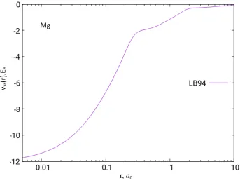
Now let us turn our attention to some model exchange potentials that are not functional
vxLB94σ =vxLDAσ −ρ1σ/3
βx2
σ
1 + 3βxσsinh−1xσ
, (.)
where β = 0.05 and xσ = |∇ρσ|/ρ4σ/3. The line integral of the LB94 potential under
di-rect orbital-scaling path involves integration over the parameter λ, which cannot be done
analytically. However, the necessary numerical integrals will be discussed in Section 2.5.
Figure 2.1: The LB94 exchange potential of the Mg atom based on HF/UGBS density
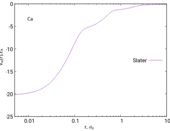
2.4.2 Slater potential
We will now apply our method to orbital-dependent potentials such as the Slater potential
and related approximations. The Slater potential is defined by [21]
vxSσ(r) = − 1
ρσ(r)
Z
|ρσ(r,r0)|2
|r−r0| dr
Figure 2.2: The Slater exchange potential of the Ca atom based on HF/UGBS density
where ρσ(r,r0) = PNi=1σ φiσ(r)φ∗iσ(r0) is the one-particle Kohn–Shamσ-spin density matrix.
In terms of scaled orbitals,
vxSσ([{φkλ}];r) =−
1
λ2ρ
σ(r)
Z |PN
j=1λ2φiσ(r)φ∗iσ(r0)|2
|r−r0| dr0
=λ2vxSσ([{φk}];r).
(.)
Using Eq. (.), we obtain
ES
xσ([{φk}];r) = N
X
i=1 Z
dr
Z 1 0
λ3vS
xσ([{φk}];r)φ∗iσ(r)φiσ(r)dλ+ c.c.
= 1 2
Z
vSxσ([{φk}];r)ρσ(r)dr
=−1 2
Z Z
|ρσ(r,r0)|2
|r−r0| dr0dr.
(.)
Comparing Eq. (.) and Eq. (1.17), we find that the energy functional obtained from the
Slater potential along the DOS path is identical toEexact
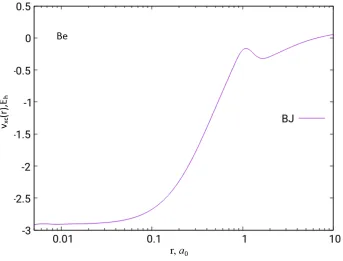
2.4.3 Becke–Johnson potential
The Becke–Johnson potential is given by [2]
vxBJσ =vxSσ+ kBJ
σ
2π , (.)
where kBJ
σ = q 10 3 τσ ρσ. We have
∇φiλ(r) =
∂λφi(r)
∂x +
∂λφi(r)
∂y +
∂λφi(r)
∂z =λ∇φi(r). (.)
So,
τσλ(r) = N
X
i=1
1
2|λ∇φiσ(r)|
2 =λ2τ
σ(r). (.)
Then, we obtain
kσλBJ(r) =
s
10 3
λ2τ
σ(r) λ2ρ
σ(r)
=kσBJ(r). (.) Using Eq. (.) and Eq. (.), we obtain the second part of the Becke–Johnson functional
EBJ−2 xσ ,
ExBJσ−2([{φkλ}];r) =
Z 1
2π
r
10
3 τσ(r)ρσ(r)dr =
Z
kBJ
σ (r)
2π ρσ(r)dr.
(.)
So,
ExBJσ([{φk}];r) = −
1 2
Z Z
|ρσ(r,r0)|2
|r−r0| dr
0dr+Z 1
2π
r
10
3 τ(r)ρ(r)dr
=Exexactσ [ρ] +
Z
kBJ
σ (r)
2π ρσ(r)dr.
The energy functional obtained from the BJ potential along DOS path is a sum ofEexact x
and an additional integral of kBJ
σ /2π times density. This additional integral is not zero for N-electron systems. As a result, the BJ–DOS functional deviates fromEexact
x .
Figure 2.3: The BJ exchange potential of the Be atom based on HF/UGBS density
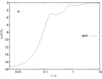
2.4.4 R¨asanen–Pittalis–Proetto potential¨
The R¨as¨anen–Pittalis–Proetto potential is given by [3]
vxRPPσ =vxSσ+ k
RPP
σ
2π , (.)
where kRPP
σ =
q 10
3
(τσ−τσW)
ρσ and τ
W
σ =|∇ρσ|2/8ρσ.
Similarly, we have
τσλW = |∇ρσ|
2
8ρσ
Using Eq. (.), we obtain
ExRPP([{φk}];r) =Exexact[ρ] +
1 2π
Z s
10 3
(τσ−τσW) ρσ
ρ(r)dr (.)
=Exexactσ [ρ] +
Z kRPP
σ (r)
2π ρσ(r)dr. (.)
The energy functional obtained from the RPP potential along DOS path has a similar
formula to the BJ–DOS functional, but the kBJ
σ under the integral is replaced by kRPPσ . For
one- or two-electron systems, as discussed in Chapter 1, kRPP
σ becomes zero, and thus, the
RPP–DOS functional becomes exact.
2.4.5 Uniform coordinate scaling
Under uniform coordinate scaling, all exchange potentials satisfy Eq. (.). Using the
following equation,
∂φiλ(r)
∂λ =
∂λ3/2φ
i(λr) ∂λ
= 3 2λ
1/2φ
i(λr) +λ3/2∇λrφi(λr)·r,
(.)
our line integral method of Eq. (.) also reduces to the Levy–Perdew virial relation, Eq.
(.).
2.5
Results and discussion
In Table 2.1, we listed total energies obtained from various orbital-dependent exchange-only
model potentials for selected atoms and molecules along the DOS and Λ paths. For the
Slater potential, the proposed DOS path gave better energies than all other paths relative
to the reference exact (HF) values. For other potentials, the Λ-path energies were most
reasonable.
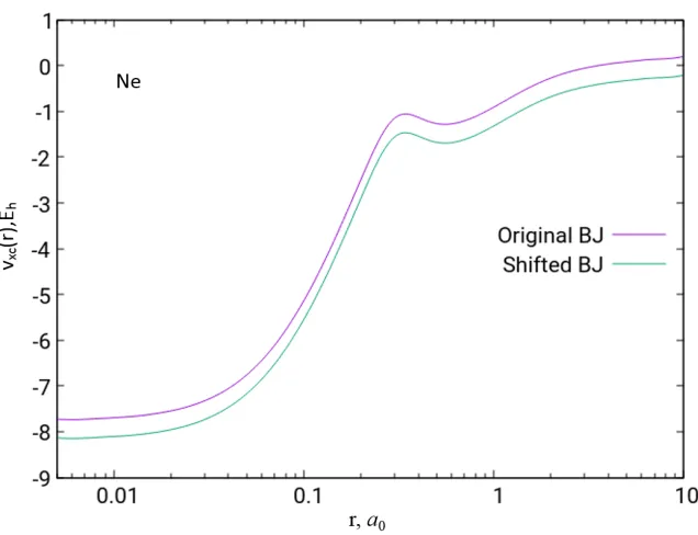
The energies obtained from the BJ potential along DOS path were significantly higher
than the exact values (see Table 2.1). One important reason for this is that the BJ potential
is upshifted [2, 15] relative to the other potentials (see Figure 2.5). We shifted vBJ
xσ, so that
the highest occupied orbital energies were equal to their HF orbital energies. In Table 2.3,
Figure 2.5: The original and shifted BJ exchange potentials of the Ne atom based on
HF/UGBS density
The RPP–DOS functional produces better results than the BJ–DOS functional. The
energies of H and He atoms obtained from RPP potentials along DOS path are the same as
the exact values (see Table 2.1), which indicates the RPP–DOS functional is exact for
one-or two-electron systems.
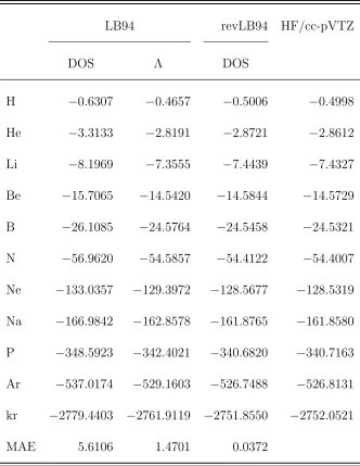
The energy expression of LB94 along DOS path involves integrals over the parameter λ,
which cannot be evaluated analytically. Therefore, we wrote a subroutine performing the
Gauss–Legendre quadrature with 256×N point grids [22, 23]. Our results were reported
in Table 2.2. We also refined the DOS-LB94 functional by changing the value of β from
0.05 to 0.025 so that it satisfied the second-order gradient expansion of GGA. The refined
LB94 functional along DOS path gave reasonable results, even better than whose from Λ
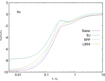
Figure 2.6: The Slater, BJ, RPP and LB94 exchange potentials of the Ne atom based on
HF/UGBS density
LB94 potentials along the DOS paths were the same as the energies reported by Gaiduk and
Staroverov along the Q path [10], which shows that for a density-dependent potential, our
line integral expressed in Eq. (.) correctly reduces to Eq. (.).
We also tested the translational invariance of the energy expression arising by integration
along the DOS path. As discussed in Section 1.6, the difference of the energies between the
displaced and original molecule is proportional to the displacement vector R. We displaced
two test molecules (H2O and HSOH) byR= (0,0,5)˚A, so that the energy differences can be
easily observed. The results reported in Table 2.4 and 2.5 show that the energies obtained by
integrating the Slater, Becke–Johnson, R¨as¨anen–Pittalis–Proetto potentials along the DOS
Figure 2.7: Structure of HSOH molecule
expressions are translationally invariant. This is to be contrasted with the energy expressions
obtained by integrating the same potentials along the Λ-paths, which are strongly
Table 2.1: Total ground-state energies (in hartrees) obtained from the Slater, Becke–Johnson, R¨as¨anen–Pittalis–Proetto
exchange-only potentials by integration along DOS and Λ paths. All values are for HF/cc-pVTZ densities (Grid=399590).
Slater Becke–Johnson RPP HF/cc-pVTZ
DOS Λ DOS Λ DOS Λ
H −0.4998 −0.4998 −0.2944 −0.5007 −0.4998 −0.4998 −0.4998
He −2.8612 −2.8612 −2.1679 −2.7857 −2.8612 −2.8612 −2.8612
Li −7.4327 −7.5389 −6.2274 −7.3771 −7.3320 −7.5522 −7.4327
Be −14.5729 −14.9126 −12.7462 −14.5317 −14.2464 −14.9416 −14.5729
B −24.5321 −25.1396 −21.9464 −24.4697 −23.8471 −25.0435 −24.5321
N −54.4007 −55.7559 −49.8808 −54.1410 −52.5111 −54.9486 −54.4007
Na −161.8580 −165.5980 −152.2437 −161.0215 −156.3319 −162.5022 −161.8580
MAE 0.0000 0.8784 2.9501 0.1903 1.2183 0.3131
Molecules at the MP2/6-31G* geometries
H2O −76.0561 −78.2515 −69.8975 −75.8002 72.8987 −76.7435 −76.0561
CH4 −40.2133 −41.4833 −35.7680 −40.4514 −38.3002 −40.6189 −40.2133
Table 2.2: Total ground-state (in hartrees) energies obtained from the LB94 and refined
LB94 exchange-only potentials by integration along DOS path and Λ paths. All values are
for HF/cc-pVTZ densities (Grid=399590).
LB94 revLB94 HF/cc-pVTZ
DOS Λ DOS
H −0.6307 −0.4657 −0.5006 −0.4998
He −3.3133 −2.8191 −2.8721 −2.8612
Li −8.1969 −7.3555 −7.4439 −7.4327
Be −15.7065 −14.5420 −14.5844 −14.5729
B −26.1085 −24.5764 −24.5458 −24.5321
N −56.9620 −54.5857 −54.4122 −54.4007
Ne −133.0357 −129.3972 −128.5677 −128.5319
Na −166.9842 −162.8578 −161.8765 −161.8580
P −348.5923 −342.4021 −340.6820 −340.7163
Ar −537.0174 −529.1603 −526.7488 −526.8131
kr −2779.4403 −2761.9119 −2751.8550 −2752.0521
Table 2.3: Total ground-state energies (in hartrees) obtained from shifted BJ potential
cal-culated for the HF/cc-pVTZ densities.
Becke–Johnson Potential HF/cc-pVTZ
DOS DOS shifted Λ
H −0.2945 −0.5000 −0.5000 −0.5000
He −2.1781 −2.8433 −2.7784 −2.8617
Li −6.2255 −6.5079 −7.3809 −7.4328
Be −12.7431 −13.2920 −14.5400 −14.5730
B −21.9504 −22.7712 −24.4755 −24.5331
Table 2.4: Total ground-state (in hartrees) energies of H2O at different positions obtained
from different exchange-only potentials by integration along DOS and Λ paths.
Position Total Energy
Slater BJ RPP HF/cc–pVTZ
DOS Λ DOS Λ DOS Λ
Initiala −76.0561 −78.2547 −69.8976 −75.8040 −72.8987 −76.7377 −76.0561
Table 2.5: Total ground-state (in hartrees) energies of HSOH at different positions obtained from different exchange-only
potentials by integration along DOS and Λ paths.
Position Total Energy
Slater BJ RPP HF/cc-pVTZ
DOS Λ DOS Λ DOS Λ
Initialc −473.5717 −483.7200 −450.2699 -472.3416 −459.3102 −475.5704 −473.5717
Displacedd −473.5717 −483.8716 −450.2699 −472.5100 −459.3102 −475.4311 −473.5717
Displacedc,d position: Both H
2O and HSOH molecules are translated by R, whereR=(0, 0, 5)
2.6
Analysis of integrating
v
xSlater+
v
xrespalong the DOS path
As discussed in Chapter 1, vexact
x is usually treated as a sum of the Slater potential and a
response correction
vxexact =vxSlater+vxresp. (.) Sincevexact
x is a functional derivative ofExexact, the line integral ofvexactx is path-independent.
Integrating vexact
x along any path should always give Exexact.
Integrating each side of Eq. (.) along the DOS path, we have
Exexact =Exexact+
N X i=1 Z dr Z 1 0
vxresp([{φkλ}];r)φiλ(r)
∂φ∗iλ(r)
∂λ dλ+ c.c.
!
, (.)
where vresp
x ([{φkλ}];r) in terms of scaled orbitals.
The terms in the brackets of the above equation should be zero
N X i=1 Z dr Z 1 0
vxresp,λφiλ(r) ∂φ∗
iλ(r)
∂λ dλ+ c.c. = 0, (.)
which indicates that the line integral of vresp
x should vanish for any system.
2.7
Summary
We developed a systematic method for turning orbital-dependent model potentials into
en-ergy functionals. As stated in Section 2.2, when vxc is not a functional derivative, the
resulting energy functional will depend on the integration path chosen. Therefore, our
pro-posed line integral expressed in Eq. (.) can be used as a method to define a new functional
approximation. The line integral along the DOS path can be applied not only to
density-dependent potentials, but also to orbital-density-dependent potentials. It is more general than the
We also applied direct orbital scaling to several model exchange potentials, and the results
were acceptable. The finding that the line integral of vresp
x should vanish may be used as a
References
[1] R. van Leeuwen and E. J. Baerends, Phys. Rev. A 49, 2421 (1994).
[2] A. D. Becke and E. R. Johnson, J. Chem. Phys. 124, 221101 (2006).
[3] E. R¨as¨anen, S. Pittalis, and C. R. Proetto, J. Chem. Phys. 132, 044112 (2010).
[4] P. R. T. Schipper, O. V. Gritsenko, S. J. A. van Gisbergen, and E. J. Baerends, J.
Chem. Phys.112, 1344 (2000).
[5] R. Armiento, S. K¨ummel, and T. K¨orzd¨orfer, Phys. Rev. B 77, 165106 (2008).
[6] F. Tran and P. Blaha, Phys. Rev. Lett. 102, 226401 (2009).
[7] M. J. T. Oliveira, E. R¨as¨anen, S. Pittalis, and M. A. L. Marques, J. Chem. Theory
Comput. 6, 3664 (2010).
[8] D. Koller, F. Tran, and P. Blaha, Phys. Rev. B 83, 195134 (2011).
[9] A. P. Gaiduk, S. K. Chulkov, and V. N. Staroverov, J. Chem. Theory Comput. 5, 699
(2009).
[10] A. P. Gaiduk and V. N. Staroverov, J. Chem. Phys. 136, 064116 (2012).
[11] R. van Leeuwen and E. J. Baerends, Phys. Rev. A 51, 170 (1995).
[12] R. van Leeuwen, O. V. Gritsenko, and E. J. Baerends, Top. Curr. Chem. 180, 107
(1996).
[14] H. Ou-Yang and M. Levy, Phys. Rev. A 44, 54 (1991).
[15] P. D. Elkind and V. N. Staroverov, J. Chem. Phys. 136, 124115 (2012).
[16] A. Karolewski, R. Armiento, and S. K¨ummel, J. Chem. Theory Comput.5, 712 (2009).
[17] A. Karolewski, R. Armiento, and S. K¨ummel, Phys. Rev. A 88, 052519 (2013).
[18] E. Engel, Chapter 2, inA Primer in Density Functional Theory, edited by C. Fiolhais,
F. Nogueira, and M. Marques, pp. 56–122, Springer, New York, NY, 2002.
[19] E. Fermi and E. Amaldi, Mem. Reale Accad. Italia 6, 117 (1934).
[20] P. W. Ayers, R. C. Morrison, and R. G. Parr, Mol. Phys. 103, 2061 (2005).
[21] J. C. Slater, Phys. Rev.81, 385 (1951).
[22] W. H. Press, S. A. Teukolsky, W. T. Vetterling, and B. P. Flannery, Integration of
Functions, inNumerical Recipes in Fortran 77: The Art of Scientific Computing Second
Edition, pp. 140–155, Cambridge University Press, New York, NY, 1992.
[23] P. J. Davis and P. Rabinowitz, Chapter 2, inMethods of Numerical Integration Second
Chapter 3
Tests for the functional derivatives
In Chapter 2, we developed a systematic method for turning orbital-dependent model
po-tentials into energy functionals. A model potential may not be a functional derivate. The
zero-force theorem may be used to test whether a given potential is not a functional derivate.
In this chapter, we focus on understanding and analyzing this theorem in application to
var-ious model potentials in calculations with finite basis sets.
3.1
The zero-force theorem
Any acceptable exchange functional should be invariant with respect to translation and
rotation of the density, and it should satisfy the Levy–Perdew virial relation [1–3]:
Ex[ρ] =− Z
ρ(r)r· ∇vx([ρ];r)dr.
Translational and rotational invariance mean that the energy of a system should not depend
on the system’s position and orientation with respect to coordinate axes. For example, if we
move a molecule from its original position byR, the densityρ(r) becomes ρ(r0) = ρ(r+R).
The exchange energy functional of the displaced molecule is
Ex[ρ0] =− Z
ρ(r+R)r· ∇rvx([ρ];r+R)dr. (.)
After substitutingr0 =r+R in Eq. (.) and replacing r0 with r we have
Ex[ρ0] =Ex[ρ] +R· Z
Since the displaced molecule should have the same energy as the undisplaced one, the second
term on the right-hand side of Eq. (.) must vanish for an arbitrary R, which requires
Z
ρ(r)∇vx([ρ];r)dr= 0 (.)
or, after integration by parts,
Z
vx([ρ];r)∇ρ(r)dr = 0. (.)
Similarly, rotational invariance requires
Z
ρ(r)r× ∇vx([ρ];r)dr= 0 (.)
or, after integration by parts,
Z
vx([ρ];r)r× ∇ρ(r)dr= 0. (.)
In electrostatics, a particle of chargeq in an electric fieldE experiences the force
F=qE. (.)
Now the electric field can be written as the gradient of a scalar potential v,
E=−∇v. (.)
Therefore, the quantity −ρ(r)∇vx(r)dr may be interpreted as the exchange force acting on
the charge ρ(r)dr. Since the electron density is the distribution of electrons for a given
system, we may define the total net exchange force on the electron density
F≡ −
Z
Translational invariance requires this force to be zero. In addition, Levy and Perdew, van
Leeuwen and Baerends independently showed that functional derivatives satisfy Eq. (.
-.) [1,4]. Eq. (.) and (.) are known as the “zero-force” and “zero-torque” theorems [3,5].
Levy and Perdew derived these conditions by employing the Hellmann–Feynman theorem [1],
whereas van Leeuwen and Baerends deduced them by using a line integral along the Λ
path [4].
If the zero-force and zero-torque theorems do not hold for an approximate vx, then
the potential is not translationally and rotationally invariant, and it is not a functional
derivative [4]. Evidence given by Gaiduk and Staroverov showed that all existing model
potentials violate these conditions and therefore have no parent energy functionals [6]. Thus,
the zero-force and zero-torque theorems can be used as tests for determining whether a given
potential is not a functional derivative and for examining the properties of a potential.
3.2
Motivation
Although Levy and Perdew, van Leeuwen and Baerends showed that functional derivatives
satisfy the zero-force test, they assumed a complete (infinite) basis set. However, in practice,
researchers use finite basis sets in any computational calculations, and it is possible that
functional derivative tests may produce different results when the calculations are done
using a finite basis set. One of our goals in this chapter is to prove that potentials derived
from explicit density functionals such as LDA and GGA satisfy the zero-force theorem in any
finite basis set. Another goal is to apply these theorems to a new type of model potentials
3.3
Basis set and basis-set limit
Most ab initio and density-functional calculations are performed using a finite set of basis
functions that is called a basis set. In DFT, specifically, a Kohn-Sham orbitalφKS
i is expressed
as a linear combination of basis functions χµ,
φKSi =X
µ
Cµiχµ, (.)
where Cµi are the coefficients determined from by solving the Kohn-Sham equations. A
Kohn-Sham orbital φKS
i can only be expanded exactly if a complete (infinite) set of basis
functions χµ is used. However, in practice, one has to use a finite basis set. Therefore, it is
important to choose a basis set so that φKS
i can be accurately represented. In this way, the
electron density can be written in terms of basis functions,
ρ=X
µ
X
ν
Pµνχµχν (.)
where P is the density matrix.
There are two types of basis functions: Slater-type orbitals (STO) and Gaussian-type
orbitals (GTO). An STO can be written as
φSTO =N xaybzce−ζr2, (.)
whereN is a normalization constant,a, b, care related to the angular momentumL=a+b+c,
while ζ determines the spatial extent of the orbital. Similarly, a GTO can be expressed as
φGTO =N xaybzce−ζr, (.)
In general, STOs give more accurate results, but they take longer to compute integrals. A
combination of n GTOs to mimic an STO is called an STO-nG basis. For example, a basis
3.3.1 Types of basis sets
The STO-3G basis set is known as a single-ζ basis set, or a minimal basis set, which indicates
that only one basis function is used to define an atomic orbital (AO). For example, N atom
has five STO-3G basis functions roughly corresponding to the AOs: 1s,2s,2px,2py,2pz.
One can increase the accuracy and flexibility of a basis set by using more than one
function to define each AO. A double-ζ basis uses two functions for each AO. Similarly, a
triple-ζ basis uses three functions. Examples of this type basis set are cc-pCVXZ, where
X=D, T, Q, 5, 6,... (D=double, T=triples, Q=quadruple, etc.). The acronym stands for
‘correlation-consistent polarized core and valence (double/triple/quadruple/etc.) zeta’.
Another type of basis sets is called a split-valence basis, which uses only one basis function
for each core AO, but two or more functions for each valence AO. The reason for this is
that core orbitals are weakly affected by their surroundings; valence orbitals, on the other
hand, must adapt to chemical bonding. Some of the commonly used split-valence basis sets
developed by Pople and co-workers are known by such names as 3-21G, 4-31G and 6-31G.
In this case, the first number represents the number of primitive Gaussians functions used
for each core AO, and the numbers after the hyphen represent the numbers of primitive
functions used for the valence functions. A universal Gaussian basis set (UGBS) is a large
basis set that uses the same set of exponents for all primitive GTOs, and only the range of
3.3.2 Basis-set limit
Generally, the more basis functions are used, the more accurate results are obtained. In
DFT calculations, a larger basis set is needed to approach the basis set limit. The basis set
limit can be extrapolated from several calculations using two or more basis sets.
Figure 3.1: Extrapolation to the basis-set limit.
Fig 3.1 is an example of an extrapolation method to estimate the energy of a given system
at the basis-set limit using the cc-pVXZ basis sets, where X=D, T, Q, 5, 6.
3.4
Zero-force condition for LDA and GGA exchange functionals
Let us focus on the zero-force condition for LDA and GGA exchange potentials. The LDA
exchange potential is written as vLDA
x = −Cx0ρ1/3(r), where Cx0 = (3/π)1/3. Ignoring the
constant Cx0, the zero-force theorem for the LDA potential requires that
Z
Applying integration by parts to the left-hand side of the above equation, we obtain
Z
ρ1/3(r)∇ρ(r)dr=ρ4/3(r)|+−∞∞−
Z
ρ(r)∇ρ1/3(r)dr. (.) Since the electron density of any finite system vanishes at infinity, the first term at the
right-hand side of the above equation is zero. Using this fact and rearranging Eq. (.), we
obtain
Z
ρ1/3(r)∇ρ(r) +ρ(r)∇ρ1/3(r)dr= 0. (.) Because
∇ρ(r) =∇[ρ1/3(r)ρ1/3(r)ρ1/3(r)] = 3[ρ2/3(r)∇ρ1/3(r)], (.) combining (.) to Eq (.), we obtain
4
Z
ρ(r)∇ρ1/3(r)dr = 0. (.) The critical step of our proof is Eq. (.). Eq. (.) holds as long as the density vanishes
at infinity. As shown in Eq. (.), every basis function has an exponential decay. Thus,
any electron density expressed in a GTO- or STO-type basis set (written as a combination of
basis functions) vanishes at infinity. Therefore, we proved that the LDA exchange potential
satisfies the zero-force theorem in any basis set as long as the density is integrable, that is,
tends to zero at infinity. All densities of finite systems are integrable.
The above analysis is also applicable to any local potential of the form
v =Cρn(r), (.)
Let us now consider a functional of the form
F[ρ] =
Z
f(r, ρ,∇ρ,∇2ρ)dr, (.)
where the function f is integrable that is, vanishes sufficiently fast at infinity. For
conve-nience, let us first analyze its gradient
∇f(r, ρ,∇ρ,∇2ρ) = ∂f
∂xi+ ∂f ∂yj+
∂f
∂zk, (.)
where i, j, k are unit vectors. Applying the chain rule to the right-hand side of the above
equation, we obtain
∂f ∂x = ∂f ∂ρ ∂ρ ∂x + ∂f ∂∇ρ · ∂∇ρ ∂x + ∂f ∂∇2ρ
∂∇2ρ
∂x . (.)
∂f ∂y and
∂f
∂z have the similar formula with respect to y and z. Therefore, we may write∇f as
∇f = ∂f
∂ρ∇ρ+
∂f ∂∇ρ · ∇
∇ρ+ ∂f
∂∇2ρ∇ ∇
2ρ, (.)
where ∇(∇2ρ) is a vector whose components are ∂2∇ρ
∂x , ∂2∇ρ
∂y , ∂2∇ρ
∂z .
According to the gradient theorem, the fact thatf(r, ρ,∇ρ,∇2ρ) vanishes at infinity implies
that
Z
∇f(r, ρ,∇ρ,∇2ρ)dr= 0. (.)
Substitution of Eq. (.) into Eq. (.) gives
Z ∂f
∂ρ∇ρ+
∂f ∂∇ρ · ∇
∇ρ+ ∂f
∂∇2ρ∇ ∇ 2ρ
dr= 0. (.)
Integrating by parts the second and third terms under the above integral and assuming that
the products of the gradients of f and ρ(r) vanish at infinity we obtain
Z ∂f ∂ρ∇ρ− ∇ · ∂f ∂∇ρ ∇ρ− ∇ ∂f ∂∇2ρ
∇2ρ