Approximation of Exchange-Correlation Potentials for Orbital- Dependent Functionals

Western University Western University

Scholarship@Western

Scholarship@Western

Electronic Thesis and Dissertation Repository

8-21-2013 12:00 AM

Approximation of Exchange-Correlation Potentials for

Approximation of Exchange-Correlation Potentials for

Orbital-Dependent Functionals

Dependent Functionals

Alexei Kananenka

The University of Western Ontario

Supervisor

Prof. Viktor N. Staroverov

The University of Western Ontario Graduate Program in Chemistry

A thesis submitted in partial fulfillment of the requirements for the degree in Master of Science © Alexei Kananenka 2013

Follow this and additional works at: https://ir.lib.uwo.ca/etd

Part of the Physical Chemistry Commons

Recommended Citation Recommended Citation

Kananenka, Alexei, "Approximation of Exchange-Correlation Potentials for Orbital-Dependent Functionals" (2013). Electronic Thesis and Dissertation Repository. 1610.

https://ir.lib.uwo.ca/etd/1610

This Dissertation/Thesis is brought to you for free and open access by Scholarship@Western. It has been accepted for inclusion in Electronic Thesis and Dissertation Repository by an authorized administrator of

APPROXIMATION OF EXCHANGE-CORRELATION

POTENTIALS FOR ORBITAL-DEPENDENT

FUNCTIONALS

(Thesis format: Integrated Article)

by

Alexei A. Kananenka

Graduate Program in Chemistry

A thesis submitted in partial fulfillment

of the requirements for the degree of

Master of Science

The School of Graduate and Postdoctoral Studies

The University of Western Ontario

London, Ontario, Canada

c

Abstract

Density-functional theory (DFT) is the most widely used method of modern com-putational chemistry. All practical implementations of DFT rely on approximations to the unknown exchange-correlation functional. These approximations may be de-vised in terms of energy functionals or effective potentials. In this thesis, several approximations of the latter type are presented.

Given a set of canonical Kohn–Sham orbitals, orbital energies, and an external potential for a many-electron system, one can invert the Kohn–Sham equations in a single step to obtain the corresponding exchange-correlation potential, vXC(r). We

show that for orbitals and orbital energies that are solutions of the Kohn–Sham equa-tions with a multiplicative vXC(r) this procedure recovers vXC(r) (in the basis set

limit), but for eigenfunctions of an orbital-specific one-electron operator it produces an orbital-averaged potential. In particular, substitution of Hartree–Fock orbitals and eigenvalues into the Kohn–Sham inversion formula is a fast way to compute the Slater potential. In the same way we obtain, for the first time, orbital-averaged exchange and correlation potentials for hybrid and kinetic-energy-density-dependent function-als. We also show how the Kohn–Sham inversion approach can be used to compute functional derivatives of explicit density functionals and to approximate functional derivatives of orbital-dependent functionals.

Motivated by the absence of an efficient practical method for computing the exact-exchange optimized effective potential (OEP) we devised the Kohn–Sham exact- exchange-correlation potential corresponding to a Hartree–Fock electron density. This potential is almost indistinguishable from the OEP and, when used as an approximation to the OEP, is vastly better than all existing models. Using our method one can obtain unambiguous, nearly exact OEPs for any finite one-electron basis set at the same low cost as the Krieger–Li–Iafrate and Becke–Johnson potentials. For all practical purposes, this solves the long-standing problem of black-box construction of OEPs in exact-exchange calculations.

Keywords: quantum chemistry, density-functional theory, model

Co-Authorship Statement

Acknowledgments

I wish to express my gratitude and admiration for my advisor, Professor Viktor Staroverov. I thank him for his guidance and support and for helping me to grow and develop as a researcher.

I would also like to thank all the past and present members of Staroverov’s group: Dr. Rogelio Cuevas-Saavedra, Amin Torabi, Sviataslau Kohut, Dan Mizzi, and Vic-toria Karner for their friendships. I am sincerely grateful to Dr. Ilya Ryabinkin and Dr. Alex Gaiduk for their guidance, but more so for their friendship which I value dearly. I enjoyed the time we spent together and appreciate all that they have made for me.

Contents

Abstract ii

Co-Authorship Statement iii

Acknowledgments iv

List of Figures vii

List of Tables viii

List of Abbreviations ix

List of Symbols x

1 Introduction 1

1.1 Kohn–Sham density-functional theory . . . 1

1.1.1 Explicit density functionals . . . 5

1.1.2 Orbital-dependent functionals . . . 6

1.1.3 Kohn–Sham method versus Hartree–Fock method . . . 7

1.2 Optimized effective potential . . . 8

1.2.1 Direct solution of the OEP equation . . . 10

1.2.2 Approximations to the OEP . . . 11

1.2.3 Model potentials as approximations to OEP . . . 12

1.3 Objectives of the research . . . 13

Bibliography . . . 13

2 Efficient construction of orbital-averaged exchange and correlation potentials by inverting the Kohn–Sham equations 18 2.1 Introduction . . . 18

2.2 Kohn–Sham inversion . . . 20

2.2.1 Inversion for multiplicative effective potentials . . . 21

2.2.2 Inversion for orbital-specific potentials . . . 23

2.3 Discussion . . . 29

2.3.2 Approximation of functional derivatives of orbital-dependent

functionals . . . 30

2.4 Conclusion . . . 33

Bibliography . . . 33

3 Accurate and efficient approximation to the optimized effective po-tential for exchange 40 3.1 Introduction . . . 40

3.2 The HFXC potential . . . 42

3.3 HFXC potential for atoms and molecules . . . 46

3.4 Conclusion . . . 52

Bibliography . . . 52

A Copyright permissions 60 A.1 APS Permission . . . 60

A.2 AIP Permission . . . 62

List of Figures

1.1 BJ, KLI and OEP potentials for Kr atom . . . 12

2.1 Exchange potentials constructed from the self-consistent LDA-X/UGBS orbitals and orbital energies in two different ways: by defini-tion (original) and by the Kohn–Sham inversion formula (reconstructed). 22

2.2 Slater potentials constructed from self-consistent Hartree–Fock UGBS orbitals by Eqs. (3.5) and (2.22). The ‘smoothened’ potential was ob-tained from the dashed curve by subtracting the LDA-X oscillation profile of Fig. 2.1. The dotted curve is almost exactly on top of the solid curve. . . 26

2.3 Various orbital-averaged exchange potentials computed in the UGBS in comparison with the numerical exchange-only OEP. Most basis-set artifacts in the reconstructed potentials were removed by subtracting the LDA-X oscillation profile of Figure 2.1 according to Eq. (2.12).. . 27

2.4 Various correlation potentials constructed as the difference vXC(r)−

vX(r), where vXC(r) andvX(r) were obtained by Kohn–Sham inversion

using the UGBS. . . 28

2.5 Model exchange potentials for the Kr atom constructed by the Kohn– Sham inversion formula using the same set of orbitals (Hartree–Fock) and various sets of self-consistent orbital eigenvalues. Basis set: UGBS. The reference OEP-X potential (black line) is from Refs. [37, 38]. . . 30

2.6 Model exchange potentials for the Kr atom constructed by the Kohn– Sham inversion formula using the same set of orbitals (TPSS-X) and various sets of self-consistent orbital eigenvalues. Basis set: UGBS. The reference OEP-X potential (black line) is from Refs. [37, 38]. . . 31

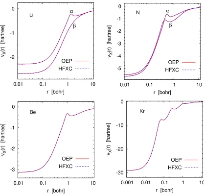
3.1 OEPs and HFXC potentials are visually indistinguishable. The same excellent agreement was observed for all atoms where comparison with OEPs was made. . . 47

3.2 HFXC potentials are perfect representations of OEPs, unlike KLI and BJ potentials. . . 48

List of Tables

List of Abbreviations

BJ — Becke–Johnson C — correlation

CEDA — common energy denominator approximation DFT — density functional theory

EXX — exact exchange

GGA — generalized gradient approximation HF — Hartree–Fock

HFXC — Hartree–Fock exchange-correlation potential H — Hartree

HOMO — highest occupied molecular orbital KLI — Krieger–Li–Iafrate

LDA — local density approximation LHF — localized Hartree–Fock LYP — Lee–Yang–Parr

OEP — optimized effective potential PBE0 — Perdew–Burke–Ernzerhof hybrid PBE — Perdew–Burke–Ernzerhof

SCF — self-consistent field S — Slater

TPSS — Tao–Perdew–Staroverov–Scuseria UGBS — universal Gaussian basis set VWN — Vosko–Wilk–Nusair

List of Symbols

Eh — atomic unit of energy (1 hartree = 2625.50 kJ mol−1= 27.2114 eV) a0 — atomic unit of length (1 bohr = 0.529177 ˚A)

N — number of electrons

Z — nuclear charge

r — position vector

ρ — electron density

γ(r,r0) — density matrix

F[ρ] — general density functional

e — general energy density

E — total energy

EXC — exchange-correlation energy EX — exchange energy

EC — correlation energy vext — external potential veff — Kohn–Sham potential

vH — Hartree (electrostatic) potential vXC — exchange-correlation potential v_XS — Slater exchange potential

vX — exchange potential φi — Kohn–Sham orbitals

Chapter 1

Introduction

1.1

Kohn–Sham density-functional theory

Density-functional theory (DFT) is a powerful approach to electronic-structure calcu-lations because it offers a high ratio between accuracy and computational cost. This makes DFT a very attractive tool for computing properties of systems with thou-sands of electrons. DFT is used by many researchers in areas as diverse as drug design, metallurgy, nanotechnology, and other fields.

DFT provides a formally exact solution to the nonrelativistic electronic many-body problem. The static Schr¨odinger equation for a system ofN interacting nonrelativistic electrons is [1]

ˆ

HΨ(x1, ...,xN) =EΨ(x1, ...,xN). (1.1)

Here, the antisymmetric N-electron wave function Ψ(x1, ...,xN) is an eigenstate of

the Hamiltonian ˆH with the energy eigenvalue E, and xi ≡ (ri, σi) are the position

and spin of theith electron.

approx-imation is given by (atomic units are used throughout the thesis) ˆ

H =−1

2

N

X

i=1

∇2

i +

N

X

i=1

vext(ri) + N

X

i<k

1

|ri−rk|

, (1.2) where vext(r) is the external potential, and 1/(|ri−rk|) represents the

electron-electron interaction. Note that, for a system with fixed nuclei, the Hamiltonian need not include the term describing the nuclear repulsion energy because this term is just a constant shift of the total energy.

Even today, solving the full many-body Schr¨odinger Eq. (1.1) remains a formidable numerical problem except for special cases such as one- and two-electron systems as well as few-electron systems with high symmetry and reduced dimensionality. The many-body wave function is a function of 3N variables, and it contains much more information than one would ever need to know about anN-electron system. Actually, we are interested in properties of the system such as the total energy, dipole moment, infrared and Raman frequencies, and polarizability. In fact, these properties are just real-valued numbers. Sometimes we also need properties that are functions of one or a few variables, for example, the single-particle probability density or the two-electron reduced density matrix. Calculating the full many-body wave function to obtain these properties seems like an unnecessarily complicated approach, especially whenN is large. This is exactly the case where DFT can be best employed.

By using DFT one can in principle obtain all properties of a many-body system exactly, without having to solve the many-body Schr¨odinger equation. The origin of DFT dates back to 1964, when Hohenberg and Kohn published [2] a basic exis-tence proof that later became known as the Hohenberg–Kohn theorem. This theorem states that the external potentialvext(r) is determined (up to a constant) by an

the number of electrons and the types and positions of the nuclei

vext(r) = − nuclei

X

A

ZA

|r−RA|

, (1.3)

whereZAis the charge of the nucleus at positionRA. Within the Kohn–Sham

frame-work of DFT, the ground-state electron density can be found by minimizing the total energy expression [2, 3]

Etot = Z

vext(r)ρ(r)dr+F[ρ], (1.4)

with respect to the density. The functional F[ρ] is universal in the sense that it is the same for any N-electron system, regardless of the external potential. Although the Hohenberg–Kohn theorem guarantees the existence of the functional Eq. (1.4), the form of this functional is unknown and must be approximated.

It was the key insight of Hohenberg and Kohn to assume that for any real (inter-acting) system with the ground-state densityρ(r) there always exists a noninteracting system with the same ground-state densityρ(r). This allows one to transform many-body Schr¨odinger equation (1.1) into a set of N one-electron Schr¨odinger equations of the form

−1

2∇

2_+v eff(r)

φi(r) = iφi(r), (1.5)

whereveff(r) is an effective Kohn–Sham potential,φi(r) are Kohn–Sham orbitals, and

iare Kohn–Sham eigenvalues. The sum of the squared occupied Kohn–Sham orbitals

gives the ground-state density of the real interacting system

ρ(r) =

N X

i=1

|φi(r)|

2

. (1.6)

ex-pression [4]

Etot=−

1 2

N

X

i=1

hφi

∇2

φ_ii+

Z

vext(r)ρ(r)dr+

1 2

Z Z

ρ(r)ρ(r0)

|r−r0_| drdr

0

+EXC[ρ], (1.7)

whereEXC is the exchange-correlation energy functional defined by EXC[ρ]≡F[ρ] +

1 2

N

X

i

hφi

∇2

φii −

1 2

Z Z _ρ(r)ρ(r0₎

|r−r0_| drdr

0

. (1.8) Equation (1.8) expresses the total energy of the real interacting system as a sum of kinetic energy for a noninteracting system (first term, usually denoted by Ts), the

attraction between the electrons and the nuclei via vext(r) (second term),

electron-electron Coulomb repulsion energy (third term), and the exchange-correlation energy

EXC which incorporates all nonclassical contributions: Pauli exchange, electron

corre-lation and the difference between the kinetic energy of real interacting system and the noninteracting model system. Now, instead of approximating the universal functional

F[ρ] we need to approximate only a small part of it—the exchange-correlation energy. It is remarkable that the Kohn–Sham method can be applied to both interact-ing and noninteractinteract-ing systems. Variation of Eq. (1.4) with respect to ρ gives the expression for the effective Kohn–Sham potential [4]

veff(r) =vext(r) + Z

ρ(r0)

|r−r0_|dr

0

+vXC(r), (1.9)

where

vXC(r) =

δEXC[ρ]

δρ(r) (1.10) is an exchange-correlation potential. Equations (1.9) and (1.10) are known as Kohn– Sham equations.

into a set of self-consistent one-electron equations with all complexity hidden invXC.

But the impact of Hohenberg–Kohn theorem on quantum physics is much more fun-damental. It represents a new paradigm of the electronic many-body problem: the wave function Ψ (a function of 3N variables) is replaced by the ground-state density

ρ(r) (a function of three variables) as the basic quantity to be calculated. However, in order to use the Kohn–Sham method in practical calculations one needs an approxi-mate form either for the exchange-correlation energy or for the exchange-correlation potential.

1.1.1

Explicit density functionals

Approximations to the exchange-correlation energy that depend on the density and its derivatives are called explicit density functionals. In 1964, Hohenberg and Kohn proposed a very simple approximate form of the exchange-correlation energy func-tional known as the local density approximation (LDA). This approximation can be derived if one assumes that exchange-correlation energy density eXC is the same as

for a homogeneous electron gas,

E_XCLDA[ρ] =

Z

eXC(ρ(r))dr, (1.11)

where the exchange-correlation energyeXC is a function ofρ(r) only. The LDA

and underestimation of bond lengths in molecules, etc.

By adding a nonlocal contribution one can overcome some of the limitations of LDA. Such functionals are called generalized gradient approximations (GGA) [5–8],

E_XCGGA[ρ] =

Z

eXC(ρ(r),∇ρ(r))dr. (1.12)

GGAs take into account deviation from the homogeneity by considering the gradient of electron density. GGAs give three times smaller errors in atomization energies than LDA. In spite of this GGAs also have limitations. For example, they do not predict stability of small anions [9–12].

1.1.2

Orbital-dependent functionals

Density-dependent approximations have served to computational chemists for many years by providing good qualitative and sometimes good quantitative results. They allow easy access to the exchange-correlation potential via functional differentiation Eq. (1.10). However, they are not perfect, so that further development is needed to improve their accuracy. The next step in designing approximations to the exchange-correlation energy (or at least to the exchange-only energy) is to consider Kohn–Sham orbitals and possibly Kohn–Sham eigenvalues as building blocks. It is beneficial for the following reasons.

functionals predict the stability of anions. Last, but not least, the exchange energy—a fundamental quantity of many-body physics is formulated in terms of orbitals,

E_Xexact =−1

4

Z dr

Z _|γ(r,r0_)|2

|r−r0_| dr

0

, (1.13) whereγ(r,r0) =PN

i=1φi(r)φ∗i(r0) is the spinless reduced density matrix.

From this point of view it should be clear that the idea of using orbital-dependent density functionals is very tempting. However, attempts to use such functionals face serious difficulties associated with deriving corresponding effective Kohn–Sham po-tentials.

1.1.3

Kohn–Sham method versus Hartree–Fock method

The Kohn–Sham density functional scheme that treats exchange energy exactly as an orbital-dependent functional of Eq. (1.13) is called exchange-only DFT. It is con-ceptually close to the Hartree–Fock method. In fact, both methods employ the same total energy functional

Etot=−

1 2

N

X

i=1

hφi

∇2

φ_ii+

Z

vext(r)ρ(r)dr+

1 2

Z Z

ρ(r)ρ(r0)

|r−r0_| drdr

0

+E_Xexact. (1.14) but the density matrixγ(r,r0) inEexact

X is different. The Kohn–Sham density matrix is

built from the Kohn–Sham orbitals. The Hartree–Fock density matrix is constructed from Hartree–Fock orbitals, eigenfunctions of the Fock operator [14,15]

ˆ

F =−1

2∇

2

where vH is the electrostatic potential and ˆK is the nonlocal Hartree–Fock exchange

potential defined by the following expression ˆ

Kφi(r) =

δEexact X δφ∗

i(r)

. (1.16)

Since Hartree–Fock and Kohn–Sham orbitals are different the Hartree–Fock exchange energy is also different from the Kohn–Sham exact-exchange energy. An important dif-ference between the Hartree–Fock and Kohn–Sham schemes is hidden in the exchange operator. The Hartree–Fock exchange operator ˆK is nonlocal (non-multiplicative) in the sense that the result of operating with it on an orbital depends on the values of all occupied orbitals everywhere in the coordinate space. The Kohn–Sham poten-tial should be local (multiplicative). Therefore the Kohn–Sham exchange (exchange-correlation) potential must also be multiplicative.

In Hartree–Fock theory, the nonlocal exchange potential is known. The exchange potential in DFT is unknown. It could have been derived from Eq. (1.13) with Kohn– Sham orbitals if it was a simple functional of an electron density. However,Eexact

X does

not depend on electron density explicitly. The Hohenberg–Kohn theorem implies that the Kohn–Sham orbitals φi(r) are functionals of the electron density. Thus we have

an implicit dependence of orbital-dependent functionals on electron density. Because of this implicit dependence one cannot evaluate the functional derivative of an orbital-dependent functional with respect to electron density. An alternative route is to derive such potential as the optimized effective potential.

1.2

Optimized effective potential

Hartree–Fock total energy expression. They treated this potential as an approxi-mation to the Hartree–Fock exchange operator and named it the optimized effective potential (OEP).

Due to the mathematical complexity of the equation proposed by Sharp and Hor-ton (OEP equation) the first solution of this equation appeared only twenty-four years later. In 1976, Talman and Shadwick [17] solved the OEP equation numerically for spherical atoms. Soon after Perdew and coworkers [18] realized that OEP is the exact-exchange potential of Kohn–Sham theory, i.e. the effective potential corresponding to exact-exchange energy (Eq. (1.13)). Today, the term OEP is generally used to denote the exchange-correlation potential of any orbital-dependent functional.

There are several different ways to derive the OEP equation and therefore differ-ent represdiffer-entations of essdiffer-entially the same equation [19]. The following OEP equa-tion is obtained by applying the chain rule for funcequa-tional derivatives to vXC(r) = δEXC[{φi}]/δρ(r) twice (“c.c.” denotes complex conjugate),

N

X

i=1

φ∗_i(r0) [vXC(r0)−uˆXC(r0)]GKS,i(r0,r)φi(r)dr0+ c.c. = 0, (1.17)

whereGKS,i(r,r0) denotes the Kohn–Sham Green’s function

GKS,i(r0,r) =

∞ X

j=1,j6=i

φj(r0)φ∗j(r)

i−j

, (1.18) and ˆuXC is an operator defined by

ˆ

uXCφi(r) =

δEXC[{φi}]

δφ∗

i(r)

com-plicated integro-differential equations. Solving these equations is a highly nontrivial task. However, there are several ways to cope with this problem. OEP equations can be solved directly or different approximations as well as model potentials may be employed.

1.2.1

Direct solution of the OEP equation

A straightforward approach to finding the OEP is to solve the OEP equation directly. The Kohn–Sham potential is expanded in a basis set and then the total energy is minimized with respect to the expansion coefficients. One such approach was devel-oped by Wu and Yang [20]. In their method, veff(r) is obtained from the following

equation:

veff(r) = vext(r) +v0(r) +

M

X

n=1

bngn(r), (1.20)

wherev0 is a fixed (Fermi–Amaldi) potential [21–23] constructed from the converged

Hartree–Fock electron density,

v0(r) = −

1

NvH(r), (1.21) {gn(r)} is a set of auxiliary primitive Gaussian-like functions, and bn are expansion

coefficients.

At convergence, the exchange part of the OEP is given by

vX(r) =

M

X

n=1

bngn(r) +v0(r)−vH(r). (1.22)

1.2.2

Approximations to the OEP

The first successful approximation to the OEP was proposed in the early 1990s by Krieger, Li, and Iafrate [25]. They introduced an approximate solution to the OEP equation for the exchange-correlation potential which is today referred to as the KLI approximation

v_XKLI(r) =vS_X(r) + 1

ρ(r)

X

i

|φi(r)|2hφi

vX−

ˆ

K

φii, (1.23)

where

vS_X(r) =− 1

2ρ(r)

Z _|

γ(r,r0)|2

|r−r0_| dr

0

(1.24) is the Slater potential. The Krieger–Li–Iafrate (KLI) potential is considerably simpler than the full OEP and it yields total energies and Kohn–Sham eigenvalues that are in close agreement with the full OEP values in many cases.

The Slater potential is a common ingredient of several others approximations to the OEP. If one assumes that the Hartree–Fock and exchange-only Kohn–Sham determinants are identical one obtains the so-called localized Hartree–Fock (LHF) approximation to the exchange potential [26]

v_XLHF(r) = v_XS(r) + 1

ρ(r)

X

i,j

φi(r)φj(r)hφi

vX−

ˆ

K

φji. (1.25)

Note that the LHF potential is more general than KLI potential because later can be obtained from LHF potential by neglecting off-diagonal elements of the Kohn–Sham Hamiltonian matrix.

The same approximation has been proposed independently by Gritsenko and Baerends in a different way under the name of “common energy denominator ap-proximation” (CEDA) [27,28].

the LHF approximation. The ELP potential minimizes the variance of operator

Pocc

i=1

vX−Kˆ

evaluated with the Hartree–Fock determinant converged in a given one-electron basis set, where ˆK is the Hartree–Fock exchange operator [31].

1.2.3

Model potentials as approximations to OEP

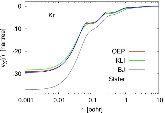
-30 -20 -10 0

0.001 0.01 0.1 1 10

vX

(r) [hartree]

r [bohr] Kr

OEP KLI BJ Slater

Figure 1.1: BJ, KLI and OEP potentials for Kr atom.

Along with direct approximations to the OEP equations there exist several model potentials for exchange. Among those perhaps the most popular was proposed by Becke and Johnson [32]:

vBJ_X (r) =vS_X(r) + kBJ

2π, (1.26)

where

kBJ=

10 3

τ ρ

1/2

, (1.27)

andτ = 1 2

PN

i=1|∇φi|2 — kinetic energy density. This potential gives accurate

exact-exchange energies via Eq. (1.13). Inclusion ofτ-dependent term makes Becke–Johnson potential closer to the OEP but due to the correction term,kBJ/2π, this potential has

1.3

Objectives of the research

Bibliography

[1] C. A. Ullrich, Time-Dependent Density Functional Theory. Concepts and Appli-cations, Oxford University Press, New York (2012).

[2] P. Hohenberg and W. Kohn, “Inhomogeneous electron gas”, Phys. Rev. 136, B864 (1964).

[3] M. Levy, “Electron densities in search of hamiltonians”, Phys. Rev. A 26, 1200 (1982).

[4] S. K¨ummel and L. Kronik, “Orbital-dependent density functionals: Theory and applications”, Rev. Mod. Phys. 80, 3 (2008).

[5] J. P. Perdew, K. Burke, and M. Ernzerhof, “Generalized gradient approximation made simple”, Phys. Rev. Lett. 77, 3865 (1996).

[6] A. D. Becke, “Density-functional exchange-energy approximation with correct asymptotic behavior”,Phys. Rev. A 38, 3098 (1988).

[9] H. B. Shore, J. H. Rose, and E. Zaremba, “Failure of the local exchange ap-proximation in the evaluation of the H− ground state”, Phys. Rev. B 15, 2858 (1977).

[10] L. A. Cole and J. P. Perdew, “Calculated electron affinities of the elements”,

Phys. Rev. A25, 1265 (1982).

[11] N. R¨osch and S. B. Trickey, “Concerning the applicability of density functional methods to atomic and molecular negative ions”, J. Chem. Phys. 106, 8940 (1997).

[12] K. Schwarz, “Instability of stable negative ions in theXα method or other local density functional schemes”,Chem. Phys. Lett. 57, 605 (1978).

[13] J. P. Perdew and A. Zunger, “Self-interaction correction to density-functional approximations for many-electron systems”,Phys. Rev. B 23, 5048 (1981). [14] A. Szabo and N. S. Ostlund, Modern Quantum Chemistry. Introduction to

Ad-vanced Electronic Structure Theory, McGraw-Hill, Inc., 1st ed. (1989).

[15] F. Jensen, Introduction to Computational Chemistry, John Wiley & Sons, New York (1999).

[16] R. T. Sharp and G. K. Horton, “A variational approach to the unipotential many-electron problem”, Phys. Rev.90, 317 (1953).

[17] J. D. Talman and W. F. Shadwick, “Optimized effective atomic central poten-tial”, Phys. Rev. A14, 36 (1976).

[18] V. Sahni, J. Gruenebaum, and J. P. Perdew, “Study of the density-gradient expansion for the exchange energy”,Phys. Rev. B 26, 4371 (1982).

[20] Q. Wu and W. Yang, “A direct optimization method for calculating density func-tionals and exchange–correlation potentials from electron densities”, J. Chem. Phys.118, 2498 (2003).

[21] E. Fermi and E. Amaldi, “Le orbite∞s degli elementi”,Mem. della Reale Accad. d’Itale 6, 117 (1934).

[22] R. G. Parr and S. K. Ghosh, “Toward understanding the exchange-correlation energy and total-energy density functionals”, Phys. Rev. A51, 3564 (1995). [23] P. W. Ayers, R. C. Morrison, and R. G. Parr, “Fermi–Amaldi model for

exchange-correlation: atomic excitation energies from orbital energy differences”, Mol. Phys.103, 2061 (2005).

[24] V. N. Staroverov, G. E. Scuseria, and E. R. Davidson, “Optimized effective poten-tials yielding Hartree–Fock energies and densities”, J. Chem. Phys.124, 141103 (2006).

[25] J. B. Krieger, Y. Li, and G. J. Iafrate, “Construction and application of an accurate local spin-polarized Kohn–Sham potential with integer discontinuity: Exchange-only theory”,Phys. Rev. A 45, 101 (1992).

[26] F. Della Sala and A. G¨orling, “Efficient localized Hartree–Fock methods as effec-tive exact-exchange Kohn–Sham methods for molecules”, J. Chem. Phys. 115, 5718 (2001).

[27] O. V. Gritsenko and E. J. Baerends, “Orbital structure of the Kohn–Sham ex-change potential and exex-change kernel and the field-counteracting potential for molecules in an electric field”, Phys. Rev. A 64, 042506 (2001).

func-tion: Application to (hyper)polarizabilities of molecular chains”,J. Chem. Phys.

116, 6435 (2002).

[29] A. F. Izmaylov, V. N. Staroverov, G. E. Scuseria, E. R. Davidson, G. Stoltz, and E. Canc`es, “The effective local potential method: Implementation for molecules and relation to approximate optimized effective potential techniques”, J. Chem. Phys.126, 084107 (2007).

[30] V. N. Staroverov, G. E. Scuseria, and E. R. Davidson, “Effective local potentials for orbital-dependent density functionals”, J. Chem. Phys. 125, 081104 (2006). [31] A. P. Gaiduk and V. N. Staroverov, “Virial exchange energies from model

exact-exchange potentials”, J. Chem. Phys. 128, 204101 (2008).

Chapter 2

Efficient construction of

orbital-averaged exchange and

correlation potentials by inverting

the Kohn–Sham equations

2.1

Introduction

The success of Kohn–Sham density-functional theory [1–3] is rooted in a highly ef-ficient approximate treatment of electron correlation. Instead of solving the many-electron Schr¨odinger equation, the Kohn–Sham scheme requires solving a one-electron equation,

−1

2∇

2

+veff(r)

φi(r) =iφi(r), (2.1)

whereveff(r) is an effective potential, such that the electron density of anN-electron

system is given by

ρ(r) =

N

X

i=1

(By φi we mean the spatial part of the ith spin-orbital.) The potential veff(r) is

normally constructed as the sum

veff(r) = v(r) +vH(r) +vXC(r), (2.3)

where v(r) is the external potential (e.g., the potential of the nuclei), vH(r) is the

Hartree (electrostatic) potential ofρ(r), andvXC(r) is the exchange-correlation

poten-tial. The termsv(r) andvH(r) are known exactly, but vXC(r) must be approximated.

Direct approximations tovXC(r) in terms of ρ orφi and possibly i (i = 1,2, . . . , N)

are known asmodel Kohn–Sham potentials [4–6].

Suppose we have a set of occupied canonical Kohn–Sham orbitals and their eigen-values. Can we recover from this information the corresponding veff(r) and hence vXC(r)? From Eq. (2.1) we have the expression

veff(r) =

1 2

∇2_φ

i(r)

φi(r)

+i, (2.4)

which is formally valid for each real φi, but in practice can be used only for the

nodeless lowest-eigenvalue orbital. Equation (2.4) has been employed for studying the exact Kohn–Sham potentials in spin-compensated two-electron systems such as the He atom and the H2 molecule [7–11]. In finite-basis-set calculations, however,

Eq. (2.4) leads to severe numerical difficulties [11–13].

Another way to extract veff(r) from {φi} and {i} is to multiply Eq. (2.1) by φ∗i,

sum overi from 1 to N, and divide through byρ. The result may be written as 1

veff(r) =

1

ρ(r)

N X i=1 1 2φ ∗

i(r)∇

2_φ

i(r) +i|φi(r)|2

. (2.5)

1_{The right-hand sides of Eqs. (2.5) and (2.7) are real despite the presence of generally} complex-valued individual terms. This is because the eigenfunctionsφi of a static Kohn–Sham Hamiltonian are either real or occur in degenerate pairs which are complex conjugates of one another, so the productsφ∗_i∇2_φ

Observe that the potential of Eq. (2.5) may be regarded as a weighted average of N

orbital-specific potentials of Eq. (2.4) with the normalized weights|φi(r)|2/ρ(r). This

observation will play a key role in situations where the potential defined by Eq. (2.4) is orbital-specific (i.e., different for different orbitals).

Equation (2.5), called here the Kohn–Sham inversion formula, is the basis of a popular numerical algorithm [14, 15] for determining the exchange-correlation poten-tial from a given electron density. It has been also used for computing the func-tional derivative of the kinetic energy funcfunc-tional [16, 17]. In this work, we show that the Kohn–Sham inversion formula may be also used to construct orbital-averaged exchange-correlation potentials for orbital-dependent functionals. In particular, we point out an efficient method for constructing the Slater exchange potential. Finally, we show how Kohn–Sham inversion can be used to obtain functional derivatives of ex-plicit density functionals without tedious calculations and to develop approximations to functional derivatives of orbital-dependent functionals.

2.2

Kohn–Sham inversion

Let us rewrite Eq. (2.5) more compactly as

veff(r) =

−τL(r) +PN_i=1i|φi(r)|2

ρ(r) , (2.6) where

τL(r) =−

1 2

N

X

i=1

φ∗_i(r)∇2_φ

i(r) (2.7)

is the Laplacian form of the kinetic energy density. From Eqs. (2.3) and (2.6),

vXC(r) =

−τL+

PN

i=1i|φi(r)|2

For a given set of occupied canonical orbitals{φi}, orbital energies{i}, and an

exter-nal potentialv(r), Eq. (2.8) specifies an exchange-correlation potential. The meaning of this potential depends on whether {φi} and {i} are solutions of a one-electron

Schr¨odinger equation with an effective multiplicativevXC(r) or with an orbital-specific

potential. Let us consider these two possibilities in detail.

2.2.1

Inversion for multiplicative effective potentials

Local density functionals such as the local density approximation (LDA) and gen-eralized gradient approximations (GGAs) such as the Perdew–Burke–Ernzerhof [18] (PBE) functional give rise to multiplicative exchange-correlation potentials defined by

vXC(r) =

δEXC[ρ]

δρ(r) . (2.9) For orbitals and orbital energies that are solutions of the Kohn–Sham equations with potentials of this type, Eq. (2.8) is clearly an identity, but only in the basis set limit [10, 11, 19]. If the Kohn–Sham equations are solved in a finite basis set and the basis-set expansions for the orbitals are substituted into Eq. (2.8), the resulting potential may strongly deviate from the original vXC(r). In particular, when the

Kohn–Sham orbitals are expanded in a Gaussian basis set, the recovered potential exhibits large spurious oscillations (especially near the nucleus) and diverges at large

r [10, 11,19].

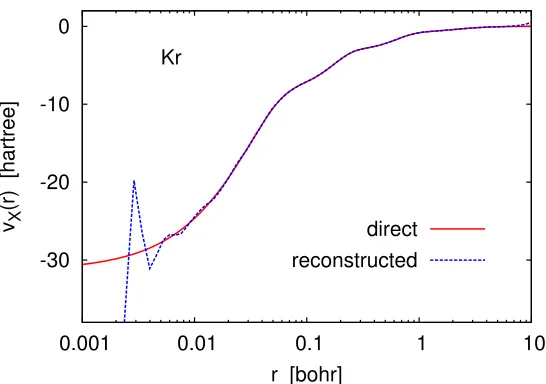
To illustrate this point, we have solved the Kohn–Sham equations for the kryp-ton atom within the exchange-only LDA (LDA-X) scheme using the universal Gaus-sian basis set [20] (UGBS) of the composition (30s,20p,14d). Then we used the self-consistent orbital and orbital energies to construct the LDA-X potential in two different ways: directly by definition,

-30 -20 -10 0

0.001 0.01 0.1 1 10

vX

(r) [hartree]

r [bohr] Kr

direct reconstructed

Figure 2.1: Exchange potentials constructed from the self-consistent LDA-X/UGBS orbitals and orbital energies in two different ways: by definition (original) and by the Kohn–Sham inversion formula (reconstructed).

where kF = (3π2ρ)1/3, and by Eq. (2.8). Figure 2.1 shows that the two potentials

coincide almost everywhere except at very small and very large r. Such artifacts are inevitable, and are even more dramatic in calculations with small and medium-size Gaussian basis sets, where the reconstructed potential may be distorted beyond recognition [10,11, 19].

Fortunately, spurious oscillations and divergences of Kohn–Sham potentials ob-tained in finite basis sets by Eq. (2.8) can be almost completely eliminated using the method proposed by us recently in Ref. [21]. This method is based on the observation that the difference

∆vosc(r) =vreconstructed(r)−voriginal(r), (2.11)

called the “oscillation profile”, is determined almost exclusively by the basis set in which vreconstructed is obtained, not the nature of the potential. For example, the

profile obtained for one potential (A) may be subtracted from a raw reconstructed potential of another approximation (B) to obtain a smoothened potential B as

vB_smooth(r) = v_{reconstructed}B (r)−∆vA_osc(r). (2.12) The easiest way to generate ∆vosc(r) for a given basis set is by using a self-consistent

LDA-X potential, which is the choice we adopt here. We will make use of this smoothening method in all subsequent examples.

Other than oscillations and divergences observed in finite-basis-set calculations, there is nothing remarkable about inverting Kohn–Sham equations with multiplicative potentials. Therefore, we will now move on to the more interesting case of orbital-specific potentials.

2.2.2

Inversion for orbital-specific potentials

Many modern density-functional approximations for the exchange-correlation energy depend on ρ(r) implicitly through the Kohn–Sham orbitals [22–24]. Examples of such orbital-dependent functionals include the exact-exchange functional, functionals with a fraction of exact exchange such as the PBE hybrid [25, 26] (PBE0), and meta-GGAs that depend on the kinetic energy density such as the Tao–Perdew–Staroverov– Scuseria [27] (TPSS) approximation. When implicit functionals are employed, it is customary to adopt the orbital-dependent Kohn–Sham formalism [28–32] in which Eq. (2.1) is replaced with a one-electron Schr¨odinger equation

−1

2∇

2

+v(r) +vH(r) + ˆuXC

φi(r) =iφi(r), (2.13)

where ˆuXC is a one-electron operator defined by

ˆ

uXCφi(r) =

δEXC[{φi}]

This operator may be either integral (as in the case of exact-exchange) or differential (e.g., for kinetic-energy-density-dependent functionals) [30, 33], but in either case it is such that (ˆuXCφi)/φi 6= (ˆuXCφj)/φj for all orbital pairs except φi = φj. Thus, if

we substitute the solutions of Eq. (2.13) into the Kohn–Sham inversion formula, we generally do not expect to obtain the functional derivativeδEXC/δρ even in the basis

set limit.

To find out the meaning of the Kohn–Sham inversion formula for solutions of Eq. (2.13), we again multiply Eq. (2.13) by φ∗_i, sum over i from 1 to N, divide both sides byρ, and write the result as

¯

vXC(r) =

−τL+

PN

i=1i|φi(r)|2

ρ(r) −v(r)−vH(r). (2.15) where

¯

vXC(r)≡

1

ρ(r)

N

X

i=1

φ∗_i(r)ˆuXCφi(r). (2.16)

By analogy with Eq. (2.8) we interpret ¯vXC(r) as an effective exchange-correlation

potential. For explicit density functionals, ¯vXC reduces to the functional derivative δEXC/δρ, but for orbital-dependent functionals Eq. (2.16) defines a model potential

that is distinct fromδEXC/δρ. Orbital-averaged potentials of this type were discussed

by Arbuznikov and coworkers [29–32].

The practical significance of Eq. (2.15) is that it can be used to construct orbital-averaged potentials ¯vXC simply by combining the standard ingredients τL,i, φi, and

vH rather than by computing the quantities ˆuXCφi. As far as we are aware, this

is equivalent to the Hartree–Fock method. The Hartree–Fock equations are

−1

2∇

2_{+v(r) +v}

H(r) + ˆK

φi(r) =iφi(r), (2.17)

in which ˆK is an integral operator defined by ˆ

Kφi(r) =

δEHF X

δφ∗_i(r) =− 1 2

Z _γ(r,r0₎

|r−r0_|φi(r

0

)dr0, (2.18) where

E_XHF =−1

4

Z dr

Z _|

γ(r,r0)|2

|r−r0_| dr

0

(2.19) is the Hartree–Fock exchange energy functional and

γ(r,r0) =

N

X

j=1

φj(r)φ∗j(r

0

) (2.20) is the one-electron reduced density matrix.

The orbital-averaged exchange potential corresponding to EHF

X is known as the

Slater potential [34],

vS_X(r) = 1

ρ(r)

N

X

i=1

φ∗_iKφˆ i =−

1 2ρ(r)

Z _|

γ(r,r0)|2

|r−r0_| dr

0

, (2.21) which is the statistical average of orbital-specific potentials [ ˆKφi(r)]/φi(r) weighted

by|φi(r)|2/ρ(r).

Direct construction of the Slater potential by Eq. (3.5) is computationally expen-sive because it involves integration over r0 for each r. Given a set of Hartree–Fock orbitals and eigenvalues, a much faster way to obtain vS

X is by using the Kohn–Sham

inversion formula,

vS_X(r) = −τL+

PN

i=1i|φi(r)| 2

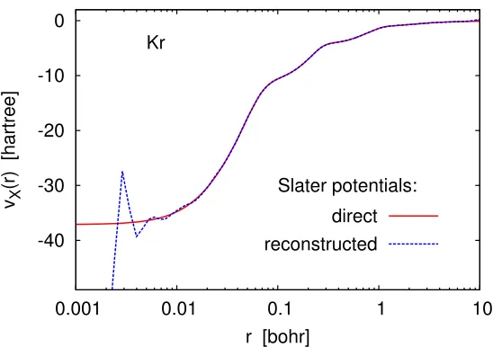
-40 -30 -20 -10 0

0.001 0.01 0.1 1 10

vX

(r) [hartree]

r [bohr] Kr

Slater potentials:

direct reconstructed

Figure 2.2: Slater potentials constructed from self-consistent Hartree–Fock UGBS orbitals by Eqs. (3.5) and (2.22). The ‘smoothened’ potential was obtained from the dashed curve by subtracting the LDA-X oscillation profile of Fig. 2.1. The dotted curve is almost exactly on top of the solid curve.

Calculation of the Slater potential by Eq. (2.22) is comparable in efficiency to insertion of the resolution of the identity into Eq. (3.5) [35], Equation (2.22) has been also discussed (in a different context) by Bulatet al.[36].

Numerical verification of Eq. (2.22) is made in Fig. 2.2, where we show Slater potentials constructed by definition (3.5) and by the Kohn–Sham inversion for-mula (2.22), before and after smoothening. The agreement between the two methods (after smoothening) is almost perfect.

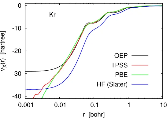
Obviously, the Kohn–Sham inversion formula can be used to construct orbital-averaged potentials for any orbital-dependent functional. Examples of orbital-averaged Hartree–Fock (Slater), TPSS and PBE0 exchange potentials are shown in Fig. 2.3. Here each ¯vX(r) was obtained by substituting into Eq. (2.15) the

-40 -30 -20 -10 0

0.001 0.01 0.1 1 10

vX

(r) [hartree]

r [bohr] Kr

OEP TPSS PBE HF (Slater)

Figure 2.3: Various orbital-averaged exchange potentials computed in the UGBS in comparison with the numerical exchange-only OEP. Most basis-set artifacts in the reconstructed potentials were removed by subtracting the LDA-X oscillation profile of Figure 2.1 according to Eq. (2.12).

and coworkers [37, 38], It is interesting to note that the PBE-X and orbital-averaged TPSS-X potentials are better approximations to the OEP than the PBE0-X poten-tial. Note also that the orbital-averaged PBE0-X potential in Fig. 2.3 appears to tend to −∞ as r → 0. This is correct because Kohn–Sham potentials derived from GGAs are in fact singular at the nucleus [7,8], A similar behavior is observed for the orbital-averaged TPSS-X potential, although to a lesser extent.

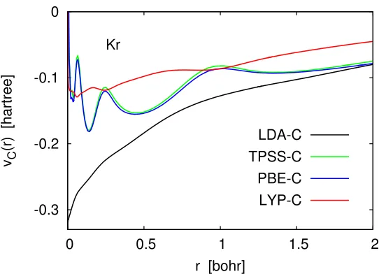
Kohn–Sham inversion can be also used to construct correlation potentials. Ex-amples of such potentials for several explicit and orbital-dependent functionals are shown in Fig. 2.4. Here each vC(r) was obtained as the difference vXC(r)−vX(r),

where vXC(r) and vX(r) were constructed using the same density. Specifically, each vXC(r) was obtained by the Kohn–Sham inversion procedure of Eq. (2.8) from the

corresponding self-consistent orbitals and orbital eigenvalues. Each vX(r) was

-0.3 -0.2 -0.1 0

0 0.5 1 1.5 2

vC

(r) [hartree]

r [bohr] Kr

LDA-C TPSS-C PBE-C LYP-C

Figure 2.4: Various correlation potentials constructed as the differencevXC(r)−vX(r),

wherevXC(r) and vX(r) were obtained by Kohn–Sham inversion using the UGBS.

computing LDA-C, PBE-C, TPSS-C, and LYP-C potentials in this way is that it requires much less work than direct evaluation of the functional derivatives of the corresponding functionals. Observe that the correlation potentials in Fig.2.4have no spurious oscillations because the basis-set artifacts present invXC(r) andvX(r) cancel

each other automatically when taking the difference.

2.3

Discussion

2.3.1

The role of orbital eigenvalues in the Kohn–Sham

in-version formula

The Kohn–Sham inversion formula (3.10) is related to another exact expression in-volving the potentialveff(r) and occupied Kohn–Sham orbitals—the differential virial

theorem for noninteracting electrons [39–41], also known as the force balance equa-tion [42, 43], In Refs. [44] and [45] we showed that this theorem can be written as

∇veff(r) = −

∇τL(r) +

PN

i=1∇2φi(r)∇φ∗i(r)

ρ(r) , (2.23) where φi are canonical Kohn–Sham orbitals. Unlike Eq. (3.10), Eq. (2.23) does not

contain orbital eigenvalues. The absence of eigenvalues in Eq. (2.23) means that the occupied Kohn–Sham orbitals alone determine, up to a vertical shift, the potential

veff(r) and, if the external potential is known, the potential vXC(r). In practice, the

presence of orbital eigenvalues in Eq. (3.10) is beneficial because it affords direct access toveff(r), whereas Eq. (2.23) yields only the gradient of veff(r).

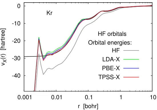
-40 -30 -20 -10 0

0.001 0.01 0.1 1 10

vX

(r) [hartree]

r [bohr] Kr

HF orbitals Orbital energies:

HF LDA-X PBE-X TPSS-X

Figure 2.5: Model exchange potentials for the Kr atom constructed by the Kohn– Sham inversion formula using the same set of orbitals (Hartree–Fock) and various sets of self-consistent orbital eigenvalues. Basis set: UGBS. The reference OEP-X potential (black line) is from Refs. [37,38].

fixed.

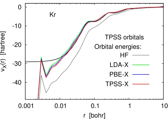
Figure 2.5 demonstrates that one can indeed obtain good approximations to the OEP by substituting into Eq. (2.15) a set of Hartree–Fock orbitals and OEP-like orbital energies obtained from LDA-X or TPSS-X calculations. This approach works because the LDA-X and TPSS-X orbital energies are closer to the corresponding OEP eigenvalues than the Hartree–Fock energies. Conversely, one can start with a good approximation to the OEP (e.g., the orbital-averaged TPSS-X potential) and turn it into a Slater-like potential simply by using Hartree–Fock orbital energies instead of TPSS-X eigenvalues (see Fig.2.6).

2.3.2

Approximation of functional derivatives of

orbital-dependent functionals

-40 -30 -20 -10 0

0.001 0.01 0.1 1 10

vX

(r) [hartree]

r [bohr] Kr TPSS orbitals Orbital energies: HF LDA-X PBE-X TPSS-X

Figure 2.6: Model exchange potentials for the Kr atom constructed by the Kohn– Sham inversion formula using the same set of orbitals (TPSS-X) and various sets of self-consistent orbital eigenvalues. Basis set: UGBS. The reference OEP-X potential (black line) is from Refs. [37,38].

OEP.

Following Della Sala and G¨orling, [35] we assume that the occupied eigenfunc-tions of the Kohn–Sham OEP Hamiltonian are the same as the eigenfunceigenfunc-tions of the Hartree–Fock Hamiltonian, i.e., φi = φHFi . Under this assumption, we can use the

Kohn–Sham inversion formula to approximate the OEP with the model potential

v_Xmodel= −τ

HF

L +

PN i=1i|φ

HF

i |2

ρHF −v−v

HF

H , (2.24)

where vHF

H is the Hartree potential built from the Hartree–Fock orbitals and i are

approximate eigenvalues of the OEP orbitals which at this point are unknown. Next consider a different potential constructed in the same manner as v_Xmodel but using Hartree–Fock orbitals and orbital energies. As explained in Sec. 2.2.2, this is the Slater potential built from the Hartree–Fock orbitals,

v_XS,HF = −τ

HF

L +

PN

i=1 HF

i |φHFi |2

ρHF −v−v

HF

According to Eqs. (2.24) and (2.25), the only difference between v_Xmodel and v_XS,HF is in the orbital energies. We already know that v_XS,HF is not a good approximation to the OEP, but expectv_Xmodel to be much better with a proper choice of i values.

Now let us subtract Eq. (2.25) from Eq. (2.24) and write the result as

vmodel_X (r) =vS,HF_X (r) + 1

ρHF_(r)

N

X

i=1

(i−HFi )|φ

HF

i (r)|

2_{. (2.26)}

A model exchange potential of this form (with φi in place of φHFi ) was discussed

by Nagy [48] as an equivalent of the Krieger–Li–Iafrate [49] (KLI) potential. Equa-tion (2.26) suggests that we define i as the eigenvalues of vXmodel. In that case, one

can determine them by iterative solution of the Kohn–Sham equations with vmodel

X ,

continuing until the potential is self-consistent.

The idea that led us to Eq. (2.26) can be readily extended to any orbital-dependent functional. In general, we obtain a model potential of the form

v_XCmodel(r) = ¯v_XC0 (r) + 1

ρ0_(r)

N

X

i=1

(i−0i)|φ

0

i(r)|

2_{, (2.27)}

where φ0

i and 0i are solutions of the orbital-specific Kohn–Sham Eq. (2.13), ¯v0XC

is the orbital-averaged potential built from φ0_i, and i are the eigenvalues of vmodelXC

2.4

Conclusion

We have shown that inversion of Kohn–Sham equations provides a convenient prac-tical method for computing functional derivatives of explicit density functionals and for constructing orbital-averaged potentials for orbital-dependent functionals. The orbital-averaged exchange potential ¯vX corresponding to the exact-exchange

func-tional (the Slater potential) is a crude approximation to the exchange-only OEP (the true functional derivative of the exact-exchange energy functional), but for hybrid and kinetic-energy-density-dependent functionals such as PBE0 and TPSS, the agreement between ¯vX and δEX/δρ is significantly better (see Fig. 2.3). We believe that the

orbital-averaged potentials for the PBE0 and TPSS functionals are shown in this work for the first time.

Bibliography

[1] W. Kohn and L. J. Sham, “Self-consistent equations including exchange and correlation effects”,Phys. Rev. 140, A1133 (1965).

[2] P. Hohenberg, W. Kohn, and L. Sham, “The beginnings and some thoughts on the future”, Adv. Quant. Chem. 21, 7 (1990).

[3] E. Engel and R. M. Dreizler, Density Functional Theory: An Advanced Course, Springer, Berlin, Berlin (2011).

[4] R. Leeuwen, O. V. Gritsenko, and E. J. Baerends, “Analysis and modelling of atomic and molecular Kohn–Sham potentials”, Top. Curr. Chem. 180, 107 (1996).

[5] O. Gritsenko, P. Schipper, and E. Baerends, “Approximation of the exchange-correlation Kohn–Sham potential with a statistical average of different orbital model potentials”, Chem. Phys. Lett.302, 199 (1999).

[6] V. N. Staroverov, “A family of model Kohn–Sham potentials for exact exchange”,

J. Chem. Phys. 129, 134103 (2008).

[8] C. Filippi, X. Gonze, and C. J. Umrigar, Recent Developments and Applications of Modern Density Functional Theory, Theoretical and Computational Chem-istry, Elsevier Science (1996).

[9] O. V. Gritsenko and E. J. Baerends, “Electron correlation effects on the shape of the Kohn–Sham molecular orbital”, Theor. Chem. Acc. 96, 44 (1997).

[10] P. R. T. Schipper, O. V. Gritsenko, and E. J. Baerends, “Kohn–Sham potentials corresponding to slater and gaussian basis set densities”,Theor. Chem. Acc. 98, 16 (1997).

[11] M. E. Mura, P. J. Knowles, and C. A. Reynolds, “Accurate numerical determina-tion of Kohn–Sham potentials from electronic densities: I. two-electron systems”,

J. Chem. Phys. 106, 9659 (1997).

[12] P. de Silva and T. A. Wesolowski, “Pure-state noninteracting v-representability of electron densities from Kohn–Sham calculations with finite basis sets”, Phys. Rev. A85, 032518 (2012).

[13] M. J. G. Peach, D. G. J. Griffiths, and D. J. Tozer, “On the evaluation of the non-interacting kinetic energy in density functional theory”,J. Chem. Phys.136, 144101 (2012).

[14] R. van Leeuwen and E. J. Baerends, “Exchange-correlation potential with correct asymptotic behavior”,Phys. Rev. A 49, 2421 (1994).

[15] O. V. Gritsenko, R. van Leeuwen, and E. J. Baerends, “Molecular Kohn–Sham exchange-correlation potential from the correlated ab initio electron density”,

Phys. Rev. A52, 1870 (1995).

[17] J. D. Goodpaster, N. Ananth, F. R. Manby, and T. F. Miller, “Exact nonadditive kinetic potentials for embedded density functional theory”,J. Chem. Phys. 133, 084103 (2010).

[18] J. P. Perdew, K. Burke, and M. Ernzerhof, “Generalized gradient approximation made simple”, Phys. Rev. Lett. 77, 3865 (1996).

[19] C. R. Jacob, “Unambiguous optimization of effective potentials in finite basis sets”, J. Chem. Phys. 135, 244102 (2011).

[20] E. V. R. de Castro and F. E. Jorge, “Accurate universal gaussian basis set for all atoms of the periodic table”, J. Chem. Phys. 108, 5225 (1998).

[21] A. P. Gaiduk, I. G. Ryabinkin, and V. N. Staroverov, “Removal of basis-set artifacts in Kohn–Sham potentials recovered from electron densities”, J. Chem. Theory and Comput. accepted (2013).

[22] T. Grabo, T. Kreibich, S. Kurth, and E. K. U. Gross, Strong Coulomb Corre-lations in Electronic Structure CalcuCorre-lations: Beyond the Local Density

Approx-imation, Advances in Condensed Matter Science, Gordon and Breach Science Publishers (2000).

[23] E. Engel, A Primer in Density Functional Theory, Lecture Notes in Physics, Springer (2003).

[24] S. K¨ummel and L. Kronik, “Orbital-dependent density functionals: Theory and applications”, Rev. Mod. Phys. 80, 3 (2008).

[25] M. Ernzerhof and G. E. Scuseria, “Assessment of the Perdew–Burke–Ernzerhof exchange-correlation functional”, J. Chem. Phys. 110, 5029 (1999).

[27] J. Tao, J. P. Perdew, V. N. Staroverov, and G. E. Scuseria, “Climbing the den-sity functional ladder: Nonempirical meta-generalized gradient approximation designed for molecules and solids”, Phys. Rev. Lett. 91, 146401 (2003).

[28] R. Neumann, R. H. Nobes, and N. C. Handy, “Exchange functionals and poten-tials”,Mol. Phys. 87, 1 (1996).

[29] A. V. Arbuznikov, M. Kaupp, V. G. Malkin, R. Reviakine, and O. L. Malkina, “Validation study of meta-gga functionals and of a model exchange-correlation potential in density functional calculations of epr parameters”, Phys. Chem. Chem. Phys.4, 5467 (2002).

[30] A. V. Arbuznikov and M. Kaupp, “The self-consistent implementation of exchange-correlation functionals depending on the local kinetic energy density”,

Chem. Phys. Lett. 381, 495 (2003).

[31] A. V. Arbuznikov, M. Kaupp, and H. Bahmann, “From local hybrid functionals to “localized local hybrid” potentials: Formalism and thermochemical tests”, J. Chem. Phys.124, 204102 (2006).

[32] A. Arbuznikov, “Hybrid exchange correlation functionals and potentials: Con-cept elaboration”, J. Struct. Chem. 48, S1 (2007).

[33] A. D. Becke, “A density-functional approximation for relativistic kinetic energy”,

The Journal of Chemical Physics 131, 244118 (2009).

[34] J. C. Slater, “A simplification of the Hartree–Fock method”,Phys. Rev. 81, 385 (1951).

[36] F. A. Bulat, M. Levy, and P. Politzer, “Average local ionization energies in the Hartree–Fock and Kohn–Sham theories”, Phys. Chem. A 113, 1384 (2009). [37] E. Engel and S. H. Vosko, “Accurate optimized-potential-model solutions for

spherical spin-polarized atoms: Evidence for limitations of the exchange-only local spin-density and generalized-gradient approximations”, Phys. Rev. A 47, 2800 (1993).

[38] E. Engel and R. M. Dreizler, “From explicit to implicit density functionals”, J. Comput. Chem. 20, 31 (1999).

[39] R. Baltin, “Hypervirial relations between ground-state particle density, kinetic energy density, and potential in three dimensions”,Phys. Lett. A117, 317 (1986). [40] A. Holas and N. H. March, “Exact exchange-correlation potential and approx-imate exchange potential in terms of density matrices”, Phys. Rev. A 51, 2040 (1995).

[41] A. Holas and N. H. March, “Exact theorems concerning noninteracting kinetic energy density functional in d dimensions and their implications for gradient expansions”, Int. J. Quantum Chem. 56, 371 (1995).

[42] N. March, “Localization via density functionals”, Top. Curr. Chem. 203, 201 (1999).

[43] V. Sahni,Quantal Density Functional Theory, Springer, Berlin (2004).

[44] I. G. Ryabinkin and V. N. Staroverov, “Determination of Kohn–Sham effective potentials from electron densities using the differential virial theorem”,J. Chem. Phys.137, 164113 (2012).

density and external potential for systems of interacting and noninteracting elec-trons”,Int. J. Quant. Chem. 113, 1626 (2013).

[46] A. G¨orling and M. Ernzerhof, “Energy differences between Kohn–Sham and Hartree–Fock wave functions yielding the same electron density”, Phys. Rev. A 51, 4501 (1995).

[47] A. Holas and N. March, “Exchange and correlation in density functional theory of atoms and molecules”,Top. Curr. Chem. 180, 57 (1996).

[48] A. Nagy, “Alternative derivation of the Krieger–Li–Iafrate approximation to the optimized-effective-potential method”,Phys. Rev. A 55, 3465 (1997).

[49] J. B. Krieger, Y. Li, and G. J. Iafrate, “Construction and application of an accurate local spin-polarized Kohn–Sham potential with integer discontinuity: Exchange-only theory”,Phys. Rev. A 45, 101 (1992).

Chapter 3

Accurate and efficient

approximation to the optimized

effective potential for exchange

3.1

Introduction

In this chapter we suggest an essentially exact, robust, practical method for construct-ing the optimized effective potential (OEP) [1] of the exact-exchange Kohn–Sham scheme. OEPs naturally arise in the theory of orbital-dependent functionals [2]—one of the most promising modern density-functional techniques—and are of significant practical interest because they afford qualitatively better description of molecular properties than local and semilocal approximations [1, 2].

The exchange-only OEP is defined [3] as the multiplicative potential vOEP X (r)

that minimizes the Hartree–Fock (HF) total energy expression within the Kohn– Sham scheme. Equivalently [4], the OEP is the functional derivative vOEP

den-sity. To obtain v_XOEP(r) in a formally correct manner, one has to solve the OEP integral equation [1]. Unfortunately, every attempt to do this runs into severe numer-ical difficulties because the problem is ill-posed [5] and has infinitely many solutions in finite basis sets [5, 6]. Recent advances in OEP methods [7–14] have alleviated some of these difficulties but, even today, flawless OEPs can be obtained only case by case, with painstaking effort.

In the absence of an efficient OEP solver, various approximations to the OEP have long been used as pragmatic alternatives. These include the Krieger–Li–Iafrate (KLI) [15], localized Hartree–Fock (LHF) [16], and related approximations [17–20], as well as model potentials for exact exchange [21–25], of which the Becke–Johnson (BJ) approximation [23] is the most popular. The LHF method is equivalent [20] to the common energy denominator approximation (CEDA) [17] and to the effective local potential (ELP) scheme [19].

In a parallel development, several workers studied [26–29] the HF method as a density-functional problem and occasionally observed [30, 31] that Kohn–Sham exchange-correlation potentials corresponding to HF electron densities (HFXC poten-tials for short) were very close to OEPs. However, this observation had little impact on the OEP impasse because existing methods for determining exchange-correlation potentials from densities (see, for instance, Refs. [32–36]) face the same basis-set ar-tifacts [37] and numerical challenges [38] as attempts to solve the OEP equation.

In this work, we devise a practical, artifact-free procedure which allows one to compute the HFXC potential efficiently for any atom or molecule. Then we use our method to show, on a variety of systems, that HFXC potentials are not just close but practically indistinguishable from OEPs. The significance of our approach is that it has the same reliability and computational cost as the KLI, LHF, and BJ schemes, but its accuracy is vastly superior.

τ)/ρ, where τ and τHF are the Kohn–Sham and HF kinetic energy densities, repro-duces that part of atomic shell structure of exact-exchange potentials which is missing in the KLI and LHF approximations. While searching for a rigorous explanation, we realized that we were dealing with the HFXC potential and arrived at the following argument.

3.2

The HFXC potential

Consider the HF description of a closed-shellN-electron system. The exchange energy of this system is

E_XHF =−1

4

Z dr

Z _|

γHF_(r,r0_)|2

|r−r0_| dr

0

, (3.1) where γHF_(r,r0_{) =} PN

i=1φHFi (r)φ

HF∗

i (r

0_{) is the spinless reduced density matrix and} φHF_i is the spatial part of the ith canonical HF spin-orbital. The HF electron density is given by ρHF(r) = PN

i=1|φ HF

i (r)|2. The orbitals φHFi are the lowest-eigenvalue

solutions of the HF equations

−1

2∇

2 _{+v(r) +v}

H(r) + ˆK

φHF_i (r) =_iHFφHF_i (r), (3.2) where v(r) is the external potential (e.g., the potential of the nuclei), vH(r) = R

ρHF_(r0_)|r−r0_|−1_dr0 _{is the Hartree (electrostatic) potential of ρ}HF_{(r), and ˆK is the}

Fock exchange operator defined by ˆ

KφHF_i (r) = δE

HF X δφHF∗

i (r)

=−1

2

Z

γHF(r,r0)

|r−r0_| φ

HF

i (r

0

ρHF. The result is

τ_LHF

ρHF +v+vH+v HF S = 1 ρHF N X i=1

HF_i |φHF_i |2_{, (3.4)}

where τHF

L (r) = −12 PN

i=1φ HF*

i (r)∇2φHFi (r) is the Laplacian form of the HF kinetic

energy density and

v_SHF(r) = − 1

2ρHF_(r) Z _|

γHF(r,r0)|2

|r−r0_| dr

0

. (3.5) is the Slater potential (the orbital-averaged ˆK operator) [39] built from the HF or-bitals. The quantity on the right-hand side of Eq. (3.4) is known as the HF average local ionization energy [40],

¯

IHF(r) = 1

ρHF_(r)

N

X

i=1

HF_i |φHF_i (r)|2_{. (3.6)}

Note thatτ_LHF=τHF− 1 4∇

2_ρHF_{, where} τHF(r) = 1

2

N

X

i=1

|∇φHF_i (r)|2 _(3.7)

is the positive-definite form of the HF kinetic energy density. In practical calculations, it is much better to deal withτHF than with τ_LHF because the former is always finite, whereas the latter becomes infinite at the nuclei. With these definitions we rewrite Eq. (3.4) as

τHF ρHF −

1 4

∇2_ρHF

ρHF +v+vH+v HF S = ¯I

HF_{. (3.8)}

Now, let us pose the following problem: Find the multiplicative exchange-correlation potential of the Kohn–Sham scheme which generates the same electron density as the HF method. This HFXC potential, vHF

Sham equations

−1

2∇

2_{+v(r) +v}

H(r) +vXCHF(r)

φi(r) = iφi(r), (3.9)

where v and vH are the same as in Eq. (3.2) and the eigenfunctionsφi are such that

ρ(r)≡PN

i=1|φi(r)|2 =ρHF(r). An important point here is that the equality ρ=ρHF

does not imply that φi =φiHF. In fact, the canonical orbitals φi and φHFi are known

to be slightly different [28]. To find vHF

XC(r), we perform the same manipulations on Eq. (3.9) that led from

Eq. (3.2) to Eq. (3.8) and arrive at

τ ρ −

1 4

∇2_ρ

ρ +v+vH+v HF

XC = ¯I, (3.10)

whereτ(r) = 1₂PN

i=1|∇φi(r)|

2 _{is the positive-definite Kohn–Sham kinetic energy}

den-sity, and

¯

I(r) = 1

ρ(r)

N

X

i=1

i|φi(r)|2 (3.11)

is the Kohn–Sham average local ionization energy. Finally, we subtract Eq. (3.8) from (3.10) and write

v_XCHF(r) = v_SHF(r) + ¯I(r)−I¯HF(r) + τ

HF_(r) ρHF_(r) −

τ(r)

ρ(r), (3.12) whereρ=ρHF_{, but τ 6=τ}HF _{and ¯I 6= ¯I}HF_.

Equation (3.12) is the key result of this work. It gives the HFXC potential exactly (in a complete basis). Analogous but less practical expressions forv_XCHFwere presented earlier in Refs. [41–43].

We propose to treat Eq. (3.12) as the definition of a model Kohn–Sham potential for exact exchange. To turn this definition into a practical method we observe that ¯I

and τ are determined by vHF

has to be solved iteratively. The algorithm we suggest is as follows.

1. Perform an HF calculation on the system of interest and construct ρHF_{, v}HF S , τHF_{, and ¯I}HF_.

2. Choose an initial guess for the occupied Kohn–Sham orbitals {φi} and their

eigenvalues {i} (e.g., HF orbitals and orbital energies).

3. Shift all i simultaneously to satisfy the condition N = HFN . This is needed to

ensure that vHF

XC retains the correct−1/r asymptotic behavior of vSHF.

4. Construct vHF

XC by substituting the current {φi} and {i} into Eq. (3.12). To

facilitate convergence, we found it essential to compute the terms ¯I and τ /ρ

using the density ρ=PN

i=1|φi|

2 _{rather thanρ}HF_.

5. Solve the Kohn–Sham equations (3.9) using the current vHF

XC. This gives a new

set of {φi} and {i}.

6. Return to Step 3. Iterate untilvHF

XC is self-consistent, i.e., until{φi}and {i}on

input and output agree within a desired threshold.

For polarized systems, there will be two HFXC potentials (up and spin-down) and hence two sets of all quantities except v and vH. The entire scheme

described above was implemented ingaussian 09[44].

The most computationally intensive step in the HFXC approach, as in the KLI, LHF, BJ, and related approximations, is the construction of the Slater potential. It helps that in our method the Slater potential has to be computed only once (at the start of iterations). To eliminate every possible source of errors unrelated to the HFXC approximation, here we constructed vHF

S (r) by using Eq. (3.5). For routine