Multi-Physics Parametric Modeling of Microwave Passive
Components Using Artificial Neural Networks
Shuxia Yan1, 2, Yaoqian Zhang1, 2, Xiaoyi Jin1, 2, Wei Zhang3, and Weiguang Shi1, 2, *
Abstract—In this paper, a novel multi-physics parametric modeling approach using artificial neural networks (ANNs) for microwave passive components is proposed. In the proposed approach, the ANN is used to learn the nonlinear relationships between electromagnetic (EM) behaviors and multi-physics design variables. The trained model can accurately represent the EM responses of the passive components with respect to the multi-physics input parameters. Therefore, the proposed model can provide accurate and fast prediction of EM responses using low computational cost and little time for multi-physics design. The advantage of the proposed model is demonstrated by two microwave examples: the proposed model can save about 98% computational cost compared with the EM model, and the CPU time of the proposed model is less than 0.1 s while that of the EM model needs many minutes.
1. INTRODUCTION
Parametric modeling of electromagnetic (EM) behavior has become important for EM design of microwave passive components [1, 2]. For high performance RF/microwave component and system design, we often require considerations of the operation in a real-world multi-physics environment which includes other physics domains besides the EM domain [3]. EM centric multi-physics design, which involves EM analysis coupled with the effects of multi-physics areas such as thermal and structural mechanics, is time consuming because it usually requires repetitive EM simulations with multi-physics parameters as design variables. Multi-physics parametric modeling becomes essential, which can develop parametric models to represent the EM responses as functions of multi-physics parameters [4].
Researches have been focused on multi-physics parametric modeling for microwave passive components. In [5], a multi-physics model has been constructed with finite element methods (FEMs) for Light Emitting Diode which works in different temperature and humidity environments. The authors in [6] have presented a multi-physics model of through-silicon vias with an equivalent-circuit approach. Most of the researches have used circuit methods and FEMs for multi-physics modeling of microwave passive components [7–9]. However, recently, the structure of microwave passive components has become more complex. Although the existing methods are suitable for modeling existing components, they are often time-consuming and computationally expensive for new components. New multi-physics modeling methods with high efficiency and low cost are needed urgently.
Artificial neural networks (ANNs) can be trained to learn any arbitrary nonlinear input-output relationships from corresponding data, which lead to ANNs being applied to many fields, especially in modeling area [10–12]. Recently, ANNs have been recognized as an effective vehicle for EM-based modeling and optimization in microwave area. Through an automatic training process, ANN can
Received 4 July 2018, Accepted 6 August 2018, Scheduled 20 August 2018
* Corresponding author: Weiguang Shi ([email protected]).
1 School of Electronics and Information Engineering, Tianjin Polytechnic University, Tianjin 300387, China.2Tianjin Key Laboratory
learn the relationship between EM responses and geometrical parameters. The trained model provides accurate and fast prediction for the EM behavior of microwave components with geometrical parameters as variables and can be subsequently implemented in circuit and system designs [13, 14]. However, how to develop multi-physics parametric models using ANN techniques remains an open topic.
In this paper, we propose a new multi-physics parametric modeling method using ANN for microwave passive components. In the proposed method, ANN is trained to learn the relationships between the EM behaviors and multi-physics design parameters. The trained ANN can provide an effective and fast prediction of EM responses with respect to multi-physics design parameters. The proposed multi-physics parametric model using ANN can achieve high accuracy of the EM responses using low computational cost and little time. A tunable evanescent mode cavity filter example and a four-pole waveguide filter example are used to illustrate the feasibility of the proposed multi-physics parametric modeling approach.
2. PROPOSED MULTI-PHYSICS MODEL
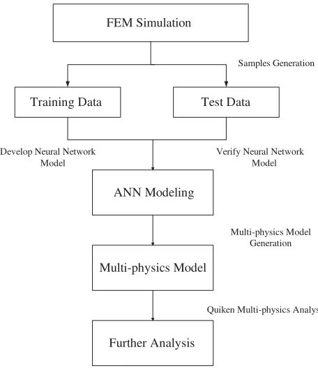
In this paper, we propose to create a multi-physics parametric model using ANN to learn the EM response of microwave passive components with respect to multi-physics design parameters. The proposed multi-physics model which learns the behavior of the components is developed through the process illustrated using the flowchart in Figure 1. Design of experiments (DOE) method [15] is used as the sampling method. The data for modeling are generated using FEM simulations. All EM data are divided into two groups: one is the training data used for training the ANN model; the other is the test data used for verifying the ANN model. In order to improve the modeling accuracy, the scaling method is used for training data [16]. The trained multi-physics parametric model can be used for fast and accurate EM centric multi-physics analysis.
We propose to use ANN as the multi-physics parametric model structure because ANN can learn the highly nonlinear relationship between input and output, and the trained ANN model is able to provide fast output solutions to the problems that they have learned. The three-layer multilayer perceptron (MLP) as one of the ANN structures, which can get the nonlinear relationship effectively and accurately,
FEM Simulation
Training Data Test Data
ANN Modeling
Multi-physics Model
Further Analysis
Samples Generation
Verify Neural Network Model
Multi-physics Model Generation
Quiken Multi-physics Analysis Develop Neural Network
Model
p
−1 pn
q
1 gx xgl xm1 xmk xf
1
y y2 yq
l l+1
1 3 2 1 2 1 Layer 3 (Output Layer) Layer 2 (Output Layer) Layer 1 (Output Layer)
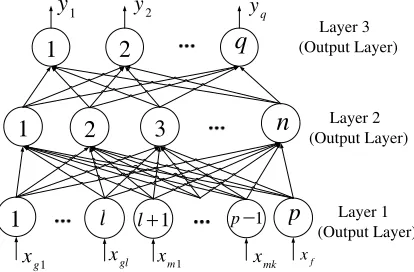
Figure 2. The proposed multi-physics parametric model using ANN.
is proposed to be used in this paper. For ANN modeling, letxbe a set including all the input variables of a given passive component, which is divided into geometrical parameters xg, multi-physics parameters
xm and frequencyxf. Letybe a set including all the output responses of the given passive component, which represents the EM behavior of the multi-physics problem. The ANN structure of the proposed multi-physics parametric model is illustrated in Figure 2. Layer 1 is the input layer (x), which receives the external inputs including xg,xm and xf by the input neurons. Layer 2 is a hidden layer of the neural network, which handles xg,xm and xf according to activation functions. Based on the neural network model in Figure 2, we propose to use the sigmoid function as the activation function for the hidden neurons, which is a smooth switch function and can be defined as
σ(γ) = 1
1 +e−γ, (1)
Layer 3 is the output layer (y), which represents the output responses of the proposed model. In Figure 2, p and q represent the numbers of input and output neurons, respectively. l and k represent the numbers ofxg and xm, respectively, i.e.,l+k=p−1. nrepresents the number of hidden neurons, which is determined during the ANN training.
For the sake of perspicuity, the calculation of the proposed model is formulated as
yj = n i=1 w(2) ij σ l h=1 w(1)
hi xgh+ k+l
r=l+1
w(1)
ri xmr+w(1)pi xf+w0(1)i
+w(2)0j , (2)
where w(1)hi, wri(1) and w(1)pi are the weight parameters between the respective (hth, rth or pth) input
neuron and the ith hidden neuron, whilew(2)ij is the weight parameters between the ith neuron in the
hidden layer and thejth neuron in the output layer. w(1)0i and w0(2)j denote bias values of theith hidden neuron and the jth output neuron, respectively. Those weight parameters determine the nonlinear relationship between input and output variables.
requirements. The same error function is defined as [17]
E(w) = 1 2 T t=1 q j=1 yt
j(x,w)−ytjD(x)2, (3)
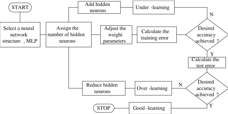
whereytj(x,w) andyjDt (w) are the EM response of the proposed model and the FEM simulations data, respectively. The subscripttis the training or test data index, andT is the total number of the training or test data. The training and test processes of the proposed multi-physics model are completed using the flowchart in Figure 3.
START
Select a neural network structure , MLP
Assign the number of hidden
neurons Adjust the weight parameters Calculate the training error Desired accuracy achieved ? Under -learning Add hidden neurons Calculate the test error Desired accuracy achieved ? Over -learning Reduce hidden neurons Good -learning STOP Y Y N N
Figure 3. The training and testing process of the proposed multi-physics model.
3. EXAMPLES
3.1. Tunable Evanescent Mode Cavity Filter
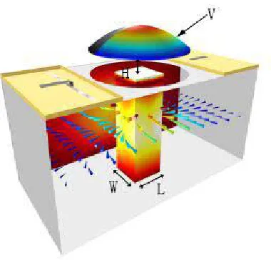
A tunable evanescent mode cavity filter [18] is used as the first example, whose structure is illustrated in Figure 4. In this example, the displacement and deformation of piezo actuator can change the magnitude of a small air gap which offers the tunability of the resonant frequency. There are 3 geometrical parameters for the filter: length (L), width (W) of the tuning post, and the gap (H) between the top of the post and the bottom side of the piezo actuator, i.e., xg= [L W H]T. It has one
multi-physics variable: bias voltage (V), which is applied on the piezo actuator, causes the deformation and displacement, i.e., xm = [V]. There is an additional input: frequency (xf), with the range from
3 GHz to 3.06 GHz. The input parameters of the proposed model for this example are defined as:
x= [L W H V f]T. The model has one output: the magnitude in decibels ofS11of the filter response, i.e., y= [S11].
In this example, the training data and testing data are generated using COMSOL Multiphysics. The range of input variables of the proposed method is shown in Table 1. The same 2025 training samples and 1600 testing samples which are sampled by DOE are used to finish the modeling process. The process of training and testing is completed using NEUROMODELERPLUS.
Figure 4. Structure of the tunable evanescent mode cavity filter.
Table 1. Definition of training and testing data.
Input variables Training data Test data Min Max Step Min Max Step
L (mm) 12 18.4 0.8 12.4 18 0.8
W (mm) 10 16.4 0.8 10.4 16 0.8
H (um) 100 148 6 103 145 6
V (V) −200 200 50 −175 175 50
Table 2. Training and test errors under different hidden neurons.
Hidden neurons Training error (%) Test error (%)
35 1.19 1.91
40 0.93 1.60
45 0.72 1.40
50 0.80 1.60
55 0.78 1.67
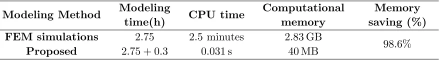
The comparison of modeling time between the FEM simulations and the proposed approach is shown in the first column of Table 3. The total modeling CPU time is 2.75 h in the COMSOL Multiphysics, while it is only about 0.35 h in the proposed method. By this comparison, it is clear that the cost in the proposed method is insignificant with a similar accuracy requirement. In other words, it is so highly efficient that the proposed approach constructs the model if the data are prepared.
(a) [12.4 11.2 109 -75]T =
x (b) [16.4 10.4 133 75]T =
x
3 3.01 3.02 3.03 3.04 3.05 3.06
-14 -12 -10 -8 -6 -4 -2 0 Frequency (GHz) |S 11 | ( d B )
COMSOL Multiphysics Data
Proposed Model
3 3.01 3.02 3.03 3.04 3.05 3.06
-27 -24 -21 -18 -15 -12 -9 -6 -3 0 Frequency (GHz) |S11 | ( d B )
COMSOL Multiphysics Data
Proposed Model
Figure 5. Comparison of the magnitude in decibels of S11 between the proposed model and the COMSOL Multiphysics data.
Table 3. Comparison of the cost and time between two modeling approaches for the tunable evanescent mode cavity filter.
Modeling Method Modeling
time(h) CPU time
Computational memory
Memory saving (%) FEM simulations 2.75 2.5 minutes 2.83 GB
98.6%
Proposed 2.75 + 0.3 0.031 s 40 MB
3.2. Four-Pole Waveguide Filter
A four-pole waveguide filter [19] is used as the second example, whose structure is illustrated in Figure 6. In this example, the displacement and deformation of four piezo actuators can change the magnitude of the small air gap which offers the tunability of the resonant frequency. There are 4 geometrical parameters for the filter: height (H1) and height (H2) of the tuning posts in the coupling windows, and height (H3) and height (H4) of the square cross section, i.e., xg = [H1 H2 H3 H4]T. It has 2 multi-physics variables: bias voltage (V1, V2), which is applied across the piezo actuator, i.e., xm= [V1 V2]T, and there is an additional input: frequency (xf), with the range from 10 GHz to 11 GHz. The input parameters of the model for this example are defined as: x= [H1 H2 H3 H4 V1 V2 f]T. The model has one output: the magnitude in decibels ofS11 of the filter response, i.e., y= [S11].
In this example, the training data and testing data are generated using COMSOL Multiphysics. The range of input variables of the proposed method is shown in Table 4. The same 8181 training samples and 1919 testing samples which are sampled by DOE are used to finish the modeling process. The process of training and testing is completed using NEUROMODELERPLUS.
Table 5 gives the training and test errors under different hidden neurons. According to Table 5, the proposed model with 55 hidden neurons has both smallest training error 1.68% and smallest test error 1.89%. Therefore, the ANN structure with 55 hidden neurons is chosen in the neural model by comparing all the errors. To show the detailed results, Figure 7 gives theS11 comparison between the COMSOL Multiphysics data and the output responses of the proposed model with respect to one set input variable. From Figure 7, the proposed model has a good agreement with the EM data.
The comparison of modeling time between the FEM simulations and the proposed approach is shown in the first column of Table 6. The total modeling CPU time is 41.75 h in the COMSOL Multiphysics while it is only about 1.2 h in the proposed method. By this comparison, it is clear that the cost in the proposed method is insignificant with a similar accuracy requirement. In other words, it is so highly efficient that the proposed approach constructs the model if the data are prepared.
Figure 6. Structure of the four-pole waveguide filter.
Table 4. Definition of training and testing data.
Input variables Training data Test data Min Max Step Min Max Step
H1 (mm) 3.04 3.44 0.05 3.065 3.415 0.05
H2 (mm) 3.10 3.50 0.05 3.125 3.475 0.05
H3 (mm) 3.52 3.84 0.04 3.54 3.82 0.04
H4 (mm) 3.28 3.52 0.03 3.295 3.505 0.03
V1 (V) −120 120 30 −105 105 30
V2 (V) −120 120 30 −105 105 30
Table 5. Training and test errors under different hidden neurons.
Hidden neurons Training error (%) Test error (%)
45 2.27 3.10
50 2.24 2.77
55 1.68 1.89
60 2.14 3.01
70 2.22 3.17
Table 6. Comparison of the cost and time between two modeling approaches for the four-pole waveguide filter.
Modeling Method Modeling
time(h) CPU time
Computational memory
Memory saving (%) FEM simulations 41.75 23.5 minutes 2.8 GB
98.2%
10 10 .2 10 .4 10 .6 10. 8 11 -28
-23 -18 -13 -8 -3 2
Frequency (GHz) |S 11
| (d
B
)
COM SOL M ultiphysics Data
Proposed M odel
Figure 7. Comparison of the magnitude in decibels of S11 between the proposed model and the COMSOL Multiphysics data with the test sample: x= [3.115 3.125 3.58 3.325 −75 −75]T.
The performance comparison of two models in practical application is illustrated in the second and third columns of Table 6. The FEM simulations model gets the corresponding output which costs the time and computational memory about 23 minutes and 2.8 GB, respectively. However, the proposed model only costs 0.058 s and 52 MB with a similar accuracy. The proposed approach can save about 98.2% computational memory compared with the FEM simulations. We can see that the proposed model provides effective and fast prediction of EM responses for passive component design in multi-physics environment. Once the proposed multi-physics model is constructed, it is used over and over again so that the benefit accumulates continuously during this process.
4. CONCLUSIONS
In this paper, an effective multi-physics parametric modeling approach using ANN for microwave passive components has been proposed. Compared with FEM simulations, the proposed approach achieves similar accuracy using less computational cost and time. The two examples results show that the more complex the component structure is, the more obvious the advantage of the proposed method is in saving calculation time and cost. The trained model can accurately represent the EM responses of the microwave passive components with respect to the multi-physics input parameters. The proposed model can be used to provide accurate and fast prediction of EM responses for multi-physics design process, which can further shorten the design cycle.
In the future, we will try to use various advanced modeling methods to construct the multi-physics model of microwave passive components. Support vector machine (SVM), space mapping (SM), and radial basis function neural network (RBF) could be useful future directions.
ACKNOWLEDGMENT
This work was supported by the National Natural Science Foundation of China (Grant No. 61601323) and the Scientific Research Project of Tianjin Education Commission (Grant No. 2017KJ088).
REFERENCES
1. Ren, L. and C. Gong, “Modified hybrid model of boost converters for parameter
identification of passive components,” IET Power Electronics, Vol. 11, 764–771, 2018,
http://dx.doi.org/10.1049/iet-pel.2017.0528.
3. Aldemir, T., R Denning, U. Catalyurek, and S. Unwin, “Methodology development for passive component reliability modeling in a multi-physics simulation environment,” United States: N. p., 2015, https://doi.org/10.2172/1214664.
4. Qian, L. X., S. l. Zheng, and H. J. Li, “Research on the multi-physics simulation
and chip implementation of piezoelectric contour mode resonator,” Symposium on
Piezo-electricity, Acoustic Waves, and Device Applications (SPAWDA), 217–221, Chengdu, 2017,
https://doi.org/10.1109/SPAWDA.2017.8340325.
5. Tang, H., D. Yang, and G. Q. Zhang, “Multi-physics modeling of LED-based luminaires under temperature and humidity environment,” 13th International Conference on Electronic Packaging Technology & High Density Packaging, 803–807, Guilin, 2012, https://doi.org/10.1109/ICEPT-HDP.2012.6474733.
6. Liu, E. X., E. P. Li, W. B. Ewe, and H. M. Lee, “Multi-physics modeling of through-silicon vias with equivalent-circuit approach,” 19th Topical Meeting on Electrical Performance of Electronic Packaging and Systems, 33–36, Austin, TX, 2010, https://doi.org/10.1109/EPEPS.2010.5642537. 7. Yang, X., Z. Wang, Y. Ren, B. Sun, and C. Qian, “Lifetime prediction based on analytical
multi-physics simulation for light-emitting diode (LED) systems,” 18th International Conference on Thermal, Mechanical and Multi-Physics Simulation and Experiments in Microelectronics and Microsystems (EuroSimE), 1–8, Dresden, 2017, https://doi.org/10.1109/EuroSimE.2017.7926233.
8. Liu, X., Q. Wu, and X. Shi, “Multi-physics analysis of waveguide filters for
wire-less communication systems,” IEEE MTT-S International Conference on Numerical
Elec-tromagnetic and Multiphysics Modeling and Optimization (NEMO), 1–2, Beijing, 2016,
https://doi.org/10.1109/NEMO.2016.7561628.
9. Yi, X., Y. Wang, M. M. Tentzeris, and R. T. Leon, “Multi-physics modeling and simulation of a slotted patch antenna for wireless strain sensing,”Structural Health Monitoring 2013: A Roadmap to Intelligent Structures — Proceedings of the 9th International Workshop on Structural Health Monitoring, IWSHM, Vol. 2, 1857–1864, 2013, https://doi.org/10.1117/12.2009233.
10. Wang, S., R. V. Rao, P. Chen, et al., “Abnormal breast detection in mammogram images by feed-forward neural network trained by jaya algorithm,” Fundamenta Informaticae, Vol. 151, Nos. 1–4, 191–211, 2017, http://dx.doi.org/10.3233/FI-2017-1487.
11. Alique, A., et al., “A Neural network-based model for the prediction of cutting force in milling process. A progress study on a real case,” IEEE International Symposium on Intelligent Control — Proceedings, Vol. 2000, 121–125, 2000, https://doi.org/10.1109/ISIC.2000.882910.
12. Fe, I. L., et al., “Automatic selection of optimal parameters based on simple soft computing methods. A case study on micro-milling processes,” IEEE Transactions on Industrial Informatics, 1–1, 2018, https://doi.org/10.1109/TII.2018.2816971.
13. Kabir, H., L. Zhang, M. Yu, P. H. Aaen, J. Wood, and Q. J. Zhang, “Smart
modeling of microwave devices,” IEEE Microwave Magazine, Vol. 11, 105–118, 2010,
https://doi.org/10.1109/MMM.2010.936079.
14. Li, X., J. Gao, and Q. J. Zhang, “Microwave noise modeling for PHEMT using artificial neural network technique,” International Journal of RF and Microwave Computer-Aided Engineering, Vol. 19, 187–196, 2009, https://doi.org/10.1002/mmce.v19:2.
15. Schmidt, S. R. and R. G. Launsby, Understanding Industrial Designed Experiments, Colorado Springs, Air Force Academy, CO, USA, 1992.
16. Zhang, Q. J. and K. C. Gupta, Neural Networks for RF and Microwave Design, Artech House, Boston, 2000.
17. Na, W., F. Feng, C. Zhang, et al., “A unified automated parametric modeling algorithm using knowledge-based neural network and l1 optimization,” IEEE Transactions on Microwave Theory
&Techniques, Vol. 99, 1–17, 2017, https://doi.org/10.1109/TMTT.2016.2630059.

![Figure 7.Comparison of the magnitude in decibels ofCOMSOL Multiphysics data with the test sample: S11 between the proposed model and the x = [3.115 3.125 3.58 3.325 − 75 − 75]T .](https://thumb-us.123doks.com/thumbv2/123dok_us/1973669.1260544/8.612.213.406.77.239/figure-comparison-magnitude-decibels-ofcomsol-multiphysics-sample-proposed.webp)
