THEORETICAL ANALYSIS OF BIT ERROR RATE OF SATELLITE COMMUNICATION IN KA-BAND UNDER SPOT DANCING AND DECREASE IN SPATIAL
COHERENCE CAUSED BY ATMOSPHERIC TURBULENCE
T. Hanada and K. Fujisaki
Department of Computer Science and Communication Engineering Graduate School of Information Science and Electrical Engineering Kyushu University
744 Motooka, Nishi-ku, Fukuoka, 819-0395, Japan
M. Tateiba
Ariake National Colleges of Technology
150 Higashihagio-Machi, Omuta, Fukuoka, 836-8585, Japan
Abstract—We study the influence of atmospheric turbulence on satellite communication by the theoretical analysis of propagation characteristics of electromagnetic waves through inhomogeneous random media. The analysis is done by using the moment of wave fields given on the basis of a multiple scattering method.
1. INTRODUCTION
In satellite communication, random fluctuation of the dielectric constant of the atmosphere affects propagation characteristics of electromagnetic waves. In particular, satellite communication in high frequencies, such as the Geostationary Earth Orbit (GEO) satellite communication in Ka-band, is significantly affected by atmospheric turbulence at low elevation angles. It causes spreading of the beam wave, decrease in the spatial coherence of received waves, spot dancing of beam waves and scintillation of received intensities. These effects result in degrade of satellite linkquality, such as the increase in bit error rate (BER).
Many studies on influences of atmospheric turbulence on satellite communication in high frequencies have been made theoretically [1–5]. In some of these studies, the influences are analyzed as the problem of wave propagation through inhomogeneous random media. The analysis is done by using the moment of wave fields given on the basis of a multiple scattering method [6, 7]. Using this method, BER of the GEO satellite communication in Ka-band under spot dancing has been analyzed numerically, where BER is derived from the integration of the average intensity on a receiving antenna [5].
However, in case that the spatial coherence of received waves is decreased and the spatial coherence radius is not much larger than a radius of the aperture of a receiving antenna, it is not enough to analyze BER by using the integration of the average intensity. In this case, BER has to be analyzed by using the mutual coherence function which includes effects of the spatial coherence of received waves.
In this paper, we numerically analyze the BER derived from the received power using the mutual coherence function on a receiving antenna as well as the BER derived from the integration of the average intensity on a receiving antenna, as shown in Reference [5]. From a result of the analysis, we consider influences of spot dancing and spatial coherence of received waves caused by atmospheric turbulence on BER of the GEO satellite communication in Ka-band at low elevation angles.
2. FORMULATION
2.1. Second Momentof Wave Fields
permeabilityµand the conductivityσ are expressed as
ε = ε0[1 +δε(r, z)] (1)
µ = µ0 (2)
σ = 0, (3)
where r = ixx +iyy (ix and iy denote the unit vectors of x and y
coordinates), ε0 and µ0 are the dielectric constant and the magnetic permeability for free space, respectively. δε(r, z) is a Gaussian random function with the properties:
δε(r, z) = 0 (4)
δε(r1, z1)·δε(r2, z2) = B(r−, z+, z−), (5) where r− = r1 − r2, z+ = (z1 + z2)/2, z− = z1 − z2 and the bracket notation·denotes an ensemble average of the quantity inside the brackets. Thus the medium fluctuates inhomogeneously in the z
direction and homogeneously in therdirection. Moreover, we assume that for anyz,
B(0, z,0)1, kl(z)1, (6)
where k = 2πf /c is the wave number for free space (f is frequency and c is velocity of light), and l(z) is the local correlation length of
δε(r, z). The medium changes little the state of polarization of the wave under the condition (6), and the present analysis can be made in the scalar approximation. In addition, the forward scattering and the small angle approximations can be applied.
We representu(r, z) as a successively forward scattered wave with exp(−jwt) time dependence in the inhomogeneous random medium. The second moment of u(r, z) is given as the solution to the moment equation [7] by:
M11(r+,r−, z) = u(r1, z)u∗(r2, z)
= 1
(2π)2
dκ+Mˆ11in(κ+,r−, z) ·exp
jκ·r−−k 2 4
z
0
dz1 z−z1
0
dz2
·D
r−−z2
kκ, z−z2− z1
2 , z1
wherer+= (r1+r2)/2,r−=r1−r2, and
D(r, z1, z2) = 2 [B(0, z1, z2)−B(r, z1, z2)] (8)
ˆ
M11in(κ+,r−, z) =
dr+M11in(r+,r−, z) exp (−jκ+·r+) (9)
M11in(r+,r−, z) = uin(r1, z)u∗in(r2, z). (10)
uin(r, z) represents a transmitted wave which is a wave function in free
space, whereδε(r, z) = 0.
2.2. Transmitted Wave Model
A transmitted wave in free space is assumed to be a Gaussian beam wave, where the transmitting antenna is located in the planez= 0 and the amplitude distribution is Gaussian with the minimum spot sizew0
at z = −z0 and w0 denotes the radius at which the field amplitude
falls to 1/eof that on the beam axis. Then, the wave field is given [8] by
uin(r, z) = (2A/π)1/2w−1exp[−(1−jp)r2/w2+j(kz−β)], (11)
whereA is constant,r=|r|and
w = w0(1 +p2)1/2 (12)
p = 2(z+z0)/(kw02) (13)
β = tan−1p. (14)
Therefore, Min
11(r+,r−, z) is given by
M11in(r+,r−, z) =
2A πw2 exp
− 2
w2r 2 ++j
2p
w2(r+·r−)−
r2−
2w2
. (15)
2.3. Correlation Function of Random Dielectric Constant
We assume that the correlation function of random dielectric constant
B(r+, z+, z−) can be expressed in terms of infinite power series in
alloverrspace as follows:
B(r−, z+, z−) = B(0, z+, z−) +
∞
i=1
a2i(z+, z−)r−2i (16)
a2i(z+, z−) =
∇2iB(r
−, z+, z−)
r−=0
where ∇ = ix∂/∂x + iy∂/∂y. From (16), the structure function
D(r−, z+, z−) defined by (8) can be also expressed in terms of the
infinite power series:
D(r−, z+, z−) =
∞
i=0
b2i(z+, z−)r−2(i+1), (18)
where
b2i(z+, z−) =−2a2(i+1)(z+, z−), i= 0,1,2, . . . . (19)
It has been already shown that ther2 term inD(r−, z+, z−) gives rise
to the ideal spot dancing of received beam waves in which the arrival position is normally distributed but each amplitude keeps the same form [6, 7].
We consider here an effect of the r2 term only in D(r−, z+, z−)
as follows:
D(r−, z+, z−) =b0(z+, z−)r−2. (20)
Substituting (20) into (7), we get the second moment under the ideal spot dancing:
M11(r+,r−, z) =
drM11in(r+−r,r−, z)
· 1 2πσ02 exp
−σ22
2 (kr−)
2
− 1 2σ02
r−jσ12kr−2
, (21)
where
σ2n=1 2
z
0
dz1
z−z1
0
dz2z22−nb0
z−z2−
z1
2, z1
, n= 0,1,2, (22)
which represents the whole effects of random dielectric constant on the second moment. Furthermore, (22) can be expressed approximately by the following equation (See Appendix A):
σ2n 1
2 z
0
dz1
∞
0
Finally, the substitution of (15) into (21) yields the second moment of Gaussian beam wave:
M11(r+,r−, z) =
dr 2A
πw2 exp
− 2
w2(r+−r) 2
+j2p w2
(r+−r)·r−
− r2−
2w2
· 1 2πσ20 exp
−r2
2σ20
exp jkσ 2 1
σ20r−·r
·exp
k2r−2
σ41
2σ02 − σ22
2
. (24)
We deduce (23) by using two type of the correlation function which are the Gaussian and the Kolmogorov models.
2.3.1. Gaussian Model
In many practical situations, a random medium may be approximated by the Gaussian correlation function:
B(r−, z+, z−) =B(z+) exp
−r2−+z−2
l2(z +)
, (25)
whereB(z+) andl(z+) are the local intensity and the correlation length
of the random medium, respectively. We then obtain
σ2n= √
π
2 z
0
dz1(z−z1)2−n
B(z1)
l(z1)
, n= 0,1,2. (26)
2.3.2. Kolmogorov Model
The Kolmogorov model is known to be a good approximation for atmospheric turbulence. Here we use the von Karman spectrum which is the modified model of the Kolmogorov spectrum. The von Karman spectrum is defined by the following equation [9]:
Φn(κ, z+) = 0.033Cn2(z+)
exp−κ2/κ2m(z+)
κ2+ 1/L2 0(z+)
11/6, 0≤κ <∞ (27)
κ2m(z+) = 5.92/l0(z+)
whereCn2(z+) is the refractive index structure constant, L0(z+) is the
outer scale of turbulence and l0(z+) is the inner scale of turbulence,
Under the assumption of a statistically homogeneous and isotropic atmosphere, the spectrum is related to the correlation function of random refractive index Bn(r−, z+, z−) by the following Fourier
transform:
Bn(r−, z+, z−) = 4π
∞
0
sinκ
r2
−+z−2
r2−+z−2
κΦn(κ, z+)dκ. (28)
Furthermore, when B(r−, z+, z−) 4Bn(r−, z+, z−) is assumed, the
correlation function of random dielectric constant is given by
B(r−, z+, z−) = 16π
∞
0
sinκ
r−2 +z−2
r2
−+z−2
κΦn(κ, z+)dκ. (29)
Using (27) and (29), we obtain
σn2 = 0.033π2
z
0
dz1(z−z1)2−nCn2(z1)
1
L0(z1)
1/3
·U
2; 7
6;
1
L20(z1)κ2m(z1)
, (30)
whereU(a, b, z) is the confluent hypergeometric function of the second kind [10].
Conducting the limit ofB(r−, z+, z−) asr−andz−approach zero
in (29), we haveCn2(z+) related with the local intensity of the random
mediaB(z+) =B(0, z+,0) as follows:
Cn2(z+) =
4π3/2·0.033
1
L0(z+)
−2/3
·U 3 2; 2 3; 1 L2
0(z+)κ2m(z+)
−1
B(z+). (31)
Therefore, (30) can be described in terms of the local intensity of the random mediaB(z1):
σn2 = √
π
4 z
0
dz1(z−z1)2−n
B(z1)
L0(z1)
U
2; 7
6;
1
L20(z1)κ2m(z1)
U 3 2; 2 3; 1 L2
0(z1)κ2m(z1)
,
2.4. Complex Degree of Coherence of Received Waves
We examine the loss of spatial coherence of received waves on the aperture of a receiving antenna by the complex degree of coherence (DOC) defined by the second moment [11]:
DOC(r, z) = M11(0,r, z)
[M11(r/2,0, z)M11(−r/2,0, z)]1/2
= exp
2
w2+ 4σ2 0
−σ02
w2(1 +p 2)
+kσ12(p+kσ21)−k
2σ2 2
2
r2
, (33)
wherer is the separation distance between received wave fields at two points on the aperture.
2.5. BER Derived from the Average Intensity
We define the BER derived from the average intensity received by an aperture antenna, whose derivation is the same as Reference [5].
We define the average intensity in free space on the receiving antenna with a Gaussian distribution of attenuation across the aperture as follows:
Iin(z) =
Sa
uin(r, z)g(r) [uin(r, z)g(r)]∗dr
=
Sa
M11in(r,0, z) [g(r)]2dr, (34)
where
g(r) = exp
−r2
σ2 a
, σ2a = 2a2 (35)
and Sa is the circular area with the aperture radius a. Similarly,
the average intensity of the received wave through the inhomogeneous random medium is defined by
I(z)=
Sa
M11(r,0, z) [g(r)]2dr. (36)
We define the energy per bitEb as the products of the intensity
and the bit time Tb; then, Eb in free space is given by
Eb=Tb·Iin(z) =Tb·
Sa
Similarly, Eb in the inhomogeneous random medium is defined by:
Eb=Tb· I(z)=Tb·
Sa
M11(r,0, z) [g(r)]2dr. (38)
We consider QPSK modulation which is very popular among satellite communication. It is known that BER in QPSK modulation is defined by:
P E= 1 2erfc Eb N0 , (39)
where erfc(x) is the complementary error function. We define the BER derived from the average intensity on a receiving antenna in order to evaluate the influence of atmospheric turbulence as follows:
P EI=
1 2erfc Eb N0
. (40)
And then, using Eb in free space obtained by (37), the BER derived
from the average intensity is expressed by:
P EI=
1 2erfc
SI·
Eb
N0
, (41)
where
SI =
Eb
Eb
= Tb· I(z)
Tb·Iin(z)
= I(z)
Iin(z)
=
Sa
M11(r,0, z) [g(r)]2dr
Sa
M11in(r,0, z) [g(r)]2dr
= 1
1 + (2σ0/w)2
1 1 + (2σ0/w)2
1
w2 +
1 σ2 a −1 ·
1−exp
−2
1 1 + (2σ0/w)2
1
w2 +
1 σ2 a a2 · 1
w2 +
1
σ2 a
1−exp
−2
1
w2 +
1 σ2 a a2 −1 . (42)
2.6. BER Derived from the Average Received Power
Here we assume a parabolic antenna as a receiving antenna. When a point detector is placed at the focus of a parabolic concentrator, the instantaneous response in the receiving antenna is proportional to the electric field strength averaged over the area of the reflector. When the aperture size is large relative to the electromagnetic wavelength, the electric field strength averaged over the area of the reflector can be described [12] by
uin=
1
Sa
Sa
uin(r, z)g(r)dr, (43)
where Sa is the circular area of a reflector with a radius a and g(r)
defined by (35) is the field distribution of attenuation across the reflector. Then, the power received by the antenna is given by
Pin(z) = Sa·
Re[uin·uin∗]
Z0
= 1
SaZ0 ·
Re
Sa
Sa
uin(r1, z)g(r1) [uin(r2, z)g(r2)]∗dr1dr2
= 1
SaZ0 ·
Re
Sa
Sa
M11in(r+,r−, z)g(r1)g(r2)dr1dr2
, (44)
where Re[x] denotes the real part of x and Z0 is the characteristic
impedance. Similarly, the average received power in the inhomoge-neous random medium is given by
P(z)= 1
SaZ0 ·
Re
Sa
Sa
M11(r+,r−, z)g(r1)g(r2)dr1dr2
. (45)
We defineEb as the products of the average received power and
the bit time Tb; then, Eb in free space is given by
Eb=Tb·Pin(z) =
Tb
SaZ0 ·
Re
Sa
Sa
M11in(r+,r−, z)g(r1)g(r2)dr1dr2
(46)
Similarly, Eb in the inhomogeneous random medium is defined by:
Eb = Tb·P(z)=
Tb
SaZ0
·Re
Sa
Sa
M11(r+,r−, z)g(r1)g(r2)dr1dr2
From the above, the BER derived from the average received power is obtained as same as the BER shown in the previous section.
P EP=
1 2erfc Eb N0 = 1
2erfc
SP·
Eb
N0
, (48)
where
SP =
Eb
Eb
= Tb· P(z)
Tb·Pin(z)
= P(z)
Pin(z)
= Re Sa Sa
M11(r+,r−, z)g(r1)g(r2)dr1dr2
Re Sa Sa
M11in(r+,r−, z)g(r1)g(r2)dr1dr2
= C0
a
0
dr1
a
0
dr2r1r2exp
C1(r12+r22)
·cosC2(r12−r22)
I0(C3r1r2) (49)
C0 =
4(w2+σ2
a)2+p2σ4a
w2σ2
a(4σa2+w2)
1 + exp
−2
1
w2 +
1 σ2 a a2
−2 exp
−
1
w2 +
1 σ2 a a2 cos p w2 1
w2 +
1 σ2 a a2
C1 = −
1 4σ20+w2
1 +2σ
2 0
w20
+2kσ
2
1(kσ12+p)
4σ20+w2 −
k2σ22
2 −
1
σ2 a
C2 =
2kσ21+p
4σ20+w2
C3 =
1 4σ2
0+w2
4σ02 w2
0
−kσ21(kσ12+p)
4σ2 0+w2
+k2σ22,
and I0(x) is the modified Bessel function of the first kind.
In case that the spatial coherence of received waves on a receiving antenna keeps constant; therefore, it is satisfied that
M11(r+,r−, z)g(r1)g(r2) = M11(r1,0, z)g(r1)g(r1), P EP shown in
3. RESULT
3.1. Model of Numerical Analysis
3.1.1. Atmospheric Turbulence
We assume a profile model of the local intensity of atmospheric turbulence as shown in Figure 1. In satellite communication in Ka-band, it is known that atmospheric turbulence mainly affects propagation characteristics of electromagnetic waves and the ionospheric turbulence can be neglected [5]. Therefore, we consider only atmospheric turbulence here. We assume the local intensity of atmospheric turbulence as a function of altitudeh from the ground as follows:
B(h) = Ba
1−
h d1
2
, 0≤h≤h1
= 0, elsewhere, (50)
where Ba is the maximum value of B(h), h1 is the altitude of
the atmosphere from the ground and d1 is the decay length of the
atmosphere.
When the elevation angle isθ, then (50) is given as a function of
z for the uplinkcommunication:
B(z) = Ba
1−
√
z2+R2+ 2zRsinθ−R
d1
2
,
0≤z≤!(h1+R)2−(Rcosθ)2−Rsinθ
= 0, elsewhere. (51)
Similarly, the local intensity for the downlinkcommunication is given by
B(z) = Ba
1−
√
z2+R2+ 2zRsinθ−R
d1
2
,
!
(R+L)2−(Rcosθ)2−!(h
1+R)2−(Rsinθ)2 ≤z
= 0, elsewhere. (52)
Figure 1. Model of atmospheric turbulence.
Table 2. Model of a satellite and a ground station.
3.1.2. Satellite and Ground Station
We assume the GEO satellite communication in Ka-band in the present analysis. The frequencies for the uplinkand the downlink communications, the elevation angle from the ground station to the satellite, and parameters about a transmitting and a receiving antenna are shown in Table 2.
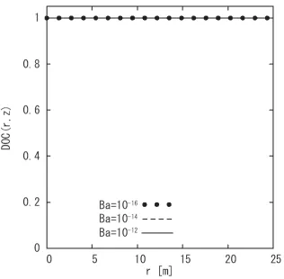
Figure 2. DOC as a function of the separation distance r for the uplinkGEO satellite communica-tion using the Gaussian model.
3.2. Numerical Analysis
3.2.1. Complex Degree of Coherence of Received Waves
Figures 2 and 3 show DOC given by (33) in the uplink communication through atmospheric turbulence which only exists near the transmitting antenna. These are analyzed by using the Gaussian and the Kolmogorov models, respectively. It is shown that DOC is nearly equal to 1; therefore, the spatial coherence radius is much larger than a radius of a receiving antenna of the GEO satellite.
Figure 4. DOC as a function of the separation distance r for the downlinkGEO satellite communi-cation using the Gaussian model.
Figure 5. Same as Figure 4 ex-cept using the Kolmogorov model.
Figures 4 and 5 show DOC in the downlinkcommunication through atmospheric turbulence which only exists near the receiving antenna. It is shown that DOC decreases; therefore, the spatial coherence radius is not much larger than a radius of a receiving antenna of the ground station. Moreover, it is shown that DOC using the Kolmogorov model decreases much more than DOC using the Gaussian model.
3.2.2. Bit Error Rate
Figures 6 and 7 show BER for the uplinkcommunication through the strong atmospheric turbulence (Ba = 10−12) using the Gaussian and
the Kolmogorov models, respectively. The dotted line shows the BER (P EI) derived from the average intensity given by (41). The solid line
Figure 6. BER in strong atmo-spheric turbulence (Ba = 10−12)
for the uplinkGEO satellite com-munication using the Gaussian model.
Figure 7. Same as Figure 6 ex-cept using the Kolmogorov model.
Figure 8. BER in strong
atmospheric turbulence (Ba =
10−12) for the downlinkGEO satellite communication using the Gaussian model.
Figure 9. Same as Figure 8 ex-cept using the Kolmogorov model.
by (48). The broken line shows BER in free space as reference. It is assumed that w0 = a= 1.2 [m]. For the Kolmogorov model, P EI is
increased as compared with BER in free space andP EP is identical to
P EI. The result of P EP =P EI was expected from Figure 3.
Figure 10. BER in strong atmospheric turbulence (Ba =
10−12) for the downlinkGEO
satellite communication in a = 2.5 [m] using the Gaussian model.
Figure 11. Same as Figure 10 ex-cept using the Kolmogorov model.
Figure 12. BER in strong atmospheric turbulence (Ba =
10−12) for the downlinkGEO satellite communication in a = 5.0 [m] using the Gaussian model.
Figure 13. Same as Figure 12 ex-cept using the Kolmogorov model.
model, it is shown that P EI is almost identical to BER in free space,
butP EP increases a little as compared with BER in free space.
It is shown for the Kolmogorov model that the larger a radius of a receiving antenna becomes, the bigger a difference betweenP EPand
P EIbecomes, because of the result shown in Figure 5.
On the other hand, for the Gaussian model, P EI and P EP are
almost same as BER in free space for both the uplinkand the downlink communication.
4. DISCUSSION
In the uplinkcommunication using the Kolmogorov model, it is shown that P EI derived from the average intensity increases in the strong
turbulence compared with BER in free space by Figure 7. The increase in BER is caused by the decrease in the average received intensity due to spot dancing of received beam waves. On the other hand, the spatial coherence radius is much larger than a radius of a receiving antenna and then the spatial coherence of received waves keeps enough on a receiving antenna as shown in Figure 3. This indicates that there are little influences of the decrease in the spatial coherence on BER. For this reason, P EP considering the spatial coherence of received
waves is almost identical to P EI derived from the average intensity
in Figure 7. After all, we find that the decrease in the average received intensity due to spot dancing causes the increase in BER for the uplink communication.
In the downlinkcommunication using the Kolmogorov model,
P EI derived from the average intensity increases little, as shown
in Figures 9, 11 and 13. This indicates that the influence of spot dancing is very small. On the other hand, the spatial coherence of received waves decrease considerably in the strong turbulence and then the spatial coherence radius is not large enough relative to a radius of a receiving antenna, as shown in Figure 5. Because of the decrease in the spatial coherence of received waves, P EP considering
the spatial coherence of received waves is increased in Figures 9, 11 and 13. Furthermore, in case that a radius of a receiving antenna is larger, the spatial coherence radius becomes smaller relative to a radius of the antenna and then the spatial coherence of received waves decreases. Therefore, the larger a radius of a receiving antenna becomes, the more P EP considering the spatial coherence of received
5. CONCLUSION
In conclusion, we find the following influences of atmospheric turbulence on the GEO satellite communication in Ka-band on the assumption that the spatial coherence of received waves decreases and spot dancing only occurs.
(i) In the uplinkcommunication, the decrease in the average intensity due to spot dancing causes the increase in BER, but the spatial coherence of received waves decreases little and there are little influences of this spatial coherence on BER.
(ii) In the downlinkcommunication, the decrease in the spatial coherence of received waves by atmospheric turbulence causes the increase in BER, but spot dancing influences little on BER. (iii) It is enough to estimate BER derived from the average intensity
(P EI) when the spatial coherence radius is much larger than a
radius of a receiving antenna. But BER derived from the average power (P EP) including with the influence of the spatial coherence
of received waves has to be considered when the spatial coherence radius is not much larger than a radius of a receiving antenna.
Furthermore, we find that the decrease in DOC and the increase in BER becomes much more in the Kolmogorov model than in the Gaussian model; therefore, the effects of atmospheric turbulence is more sensitive in the Kolmogorov model than the Gaussian model.
In this paper, we do not consider effects of scintillation of received intensities. At the next stage, we will examine effects of both spot dancing and scintillation on satellite communication. We estimate BER in atmospheric turbulence by using the average intensity or the average received power. In order to make a more actual analysis, we have to consider the probability density function (PDF) about the bit error of satellite communication. The introduction of PDF is a future problem.
ACKNOWLEDGMENT
This research was partially supported by the Ministry of Education, Science, Sports and Culture, Grant-in-Aid for Scientific Research (C), 20560359, 2008.
APPENDIX A. APPROXIMATION OF EQUATION (22)
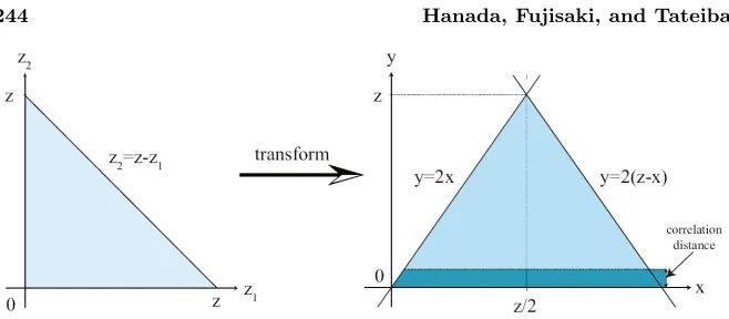
Figure A1. Range of integration forz1 andz2, and the corresponding
range of integration forx and y.
We transform the integration of (22) with respect to z1 and z2
into the difference coordinate
x = z−z2−
z1
2 (A1)
y = z1. (A2)
The transformation changes the region of the integration as shown in Figure A1. Because the appreciable values of the functionb0(x, y) exist
only for y within the correlation distance, shown by the darkshaded region in Figure A1, it follows that the limits of integration ony can be extended from 0 to ∞ without significant error. In addition, z22−n
in the integrand can be approximated by
z22−n=
z−x−y
2 2−n
(z−x)2−n, n= 0,1,2. (A3)
From the above approximations, (22) can be represented by
σn2 = 1 2
z
0
dz1
z−z1
0
dz2z22−nb0
z−z2−
z1
2, z1
1 2
z
0
dx
∞
0
dy(z−x)2−nb0(x, y), (A4)
and (23) is obtained by replacing x,y by z1,z2 in (A4)
REFERENCES
2. Fante, R. L., “Electromagnetic beam propagation in turbulent media,”Proceedings of the IEEE, Vol. 63, No. 12, 1669–1692, 1975. 3. Tateiba, M., “Analysis of antenna gain reduction due to inhomogeneous fluctuations of random media,”1984 International Symposium on Electromagnetic Compatibility, Vol. 1, 474–478, Institute of Electrical and Electronics Engineers, New York, 1984. 4. Tateiba, M. and T. Yokoi, “Analysis of antenna gain reduction due to ionospheric and atmospheric turbulence,” Proceedings of ISAP’85, 711–714, 1985.
5. Yamada, K., K. Fujisaki, and M. Tateiba, “Analysis of the bit error due to the arrival-angle fluctuation in Ka-band satellite turbulent channels,” Journal of Electromagnetic Waves and Applications, Vol. 16, No. 8, 1135–1151, 2002.
6. Tateiba, M., “Mechanism of spot dancing,”IEEE Transactions on Antennas and Propagation, Vol. 23, No. 4, 493–496, 1975.
7. Tateiba, M., “Multiple scattering analysis of optical wave propagation through inhomogeneous random media,” Radio Science, Vol. 17, No. 1, 205–210, 1982.
8. Tateiba, M., “Some useful expression for spatial coherence functions propagated through random media,” Radio Science, Vol. 20, No. 5, 1019–1024, 1985.
9. Ishimaru, A.,Wave Propagation and Scattering in Random Media, IEEE Press, 1997.
10. Zhang, S. and J. Jin, Computation of Special Functions, John Wiley & Sons, Inc., 1996.
11. Andrews, L. C. and R. L. Phillips, Laser Beam Propagation through Random Media, SPIE Press, 2005.