Symmetry Shape Prior for Object Segmentation

(1)

Western University Western University

Scholarship@Western

Electronic Thesis and Dissertation Repository

12-11-2015 12:00 AM

Symmetry Shape Prior for Object Segmentation

Xinze Liu

The University of Western Ontario

Supervisor Dr. Olga Veksler

The University of Western Ontario Graduate Program in Computer Science

A thesis submitted in partial fulfillment of the requirements for the degree in Master of Science © Xinze Liu 2015

Follow this and additional works at: https://ir.lib.uwo.ca/etd

Recommended Citation Recommended Citation

Liu, Xinze, "Symmetry Shape Prior for Object Segmentation" (2015). Electronic Thesis and Dissertation Repository. 3428.

https://ir.lib.uwo.ca/etd/3428

This Dissertation/Thesis is brought to you for free and open access by Scholarship@Western. It has been accepted for inclusion in Electronic Thesis and Dissertation Repository by an authorized administrator of

(2)

SYMMETRY SHAPE PRIOR FOR OBJECT SEGMENTATION

(Thesis format: Monograph)

by

Xinze Liu

Graduate Program in Computer Science

A thesis submitted in partial fulfillment

of the requirements for the degree of

Masters of Science

The School of Graduate and Postdoctoral Studies

The University of Western Ontario

London, Ontario, Canada

c

(3)

Abstract

Symmetry is a useful segmentation cue. We develop an algorithm for segmenting a single

symmetric object from the background. Our algorithm is formulated in the principled global

optimization framework. Thus we can incorporate all the useful segmentation cues in the global

energy function, in addition to the symmetry shape prior. We use the standard cues of regular

boundary and coherent object (background) appearance. Our algorithm consists of two stages.

The first stage, based on seam carving, detects a set of symmetry axis candidates. Symmetry

axis is detected by first finding image “seams” that are aligned with intensity gradients and

then matching them based on pairwise symmetry. The second stage formulates symmetric

object segmentation in discrete optimization framework. We choose the longest symmetry axis

as the object axis. Object symmetry is encouraged through submodular long-range pairwise

terms. These pairwise terms are submodular, so optimization with a graph cut is applicable.

We demonstrate the effectiveness of symmetry cue on a new symmetric object dataset.

Keywords: binary image segmentation, Graph cut, symmetry detection, seam carving, Grab cut

(4)

List of Figures

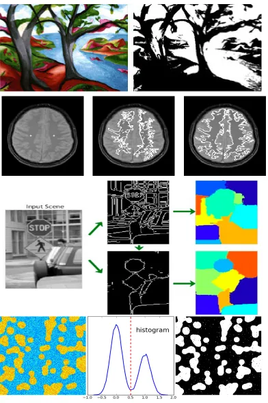
1.1 Examples for different kinds of segmentation. First row: example of

threshold-ing methods. Second row: example of region-growthreshold-ing methods. Third row:

ex-ample of boundary based methods. Bottom row: exex-ample of histogram-based

methods . . . 6

1.2 An example for disadvantage of region-growing. . . 7

1.3 Examples of segmentation based on global optimization. Top row: example of multi-label segmentation Getreuer, Pascal [17]. Left is the original image. Right is the segmentation result. Middle row: Left is user input, blue strokes are seeds for background and red strokes are seeds for object. Right is the segmentation result Boykov, Yuri Y and Jolly, Marie-Pierre [10]. Bottom row: Grabcut Rother, Carsten et al. [46]. Left is the user input with a rectangle containing the object. Right is the segmentation result. . . 8

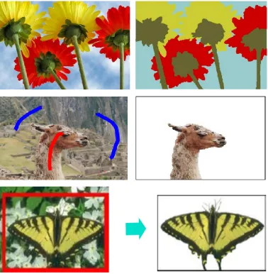
1.4 Examples of symmetric objects. . . 9

1.5 Examples for situations that may cause inaccurate results . . . 10

1.6 Examples of symmetric objects. . . 11

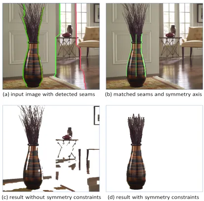
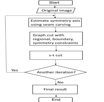
1.7 Overview of our approach in the single object case: (a) input image with most significant seams from seam carving; (b) the longest matching seams pair and the corresponding symmetry axis; (c) result initialized with (b) but without symmetry constraints; (d) result initialized with (b) with symmetry constraints. 12 1.8 The flow chart of our segmentation algorithm . . . 13

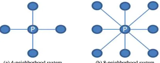
2.1 Representation of 4 and 8 neighborhood system. . . 15

2.2 An example of a cut on a graph Boykov, Yuri Y and Jolly, Marie-Pierre [10]. . . 17

2.3 The process of max flow/min cut Boykov, Yuri Y and Jolly, Marie-Pierre [10]. . 17

2.4 Hard constraints in a graph Boykov, Yuri Y and Jolly, Marie-Pierre [10]. . . 18

2.5 An example of binary segmentation using Graph cut Boykov, Yuri Y and Jolly, Marie-Pierre [10]. . . 19

2.6 Examples of Grabcut Avidan, Shai and Shamir, Ariel [3]. . . 20

(7)

2.7 An example of more user interaction Avidan, Shai and Shamir, Ariel [3], the

white curve drawn at the soldier’s helmet is the user input. . . 21

2.8 Examples of various symmetry patterns Liu, Yanxi et al. [35]. . . 25

2.9 Examples for global symmetry and local symmetry Liu, Yanxi et al. [35]. . . . 27

2.10 It is mentioned in Avidan, Shai and Shamir, Ariel [4] that seam insertion is finding and inserting the optimum seam on an enlarged image will most likely insert the same seam again and again as in (b). Inserting the seams in order of removal (c) achieves the desired 50% enlargement (d). Using two steps of seam insertions of 50% in (f) achieves better results than scaling (e). . . 31

2.11 On the left is the input image. On the right is the energy image of the input image. . . 31

3.1 The flow chart of this chapter. . . 34

3.2 Extracting symmetry axis candidates: (a) gradient magnitude energy for seam carving on the input image; (b) input image overlaid with high energy seams; (c) three matched seam subparts the corresponding symmetry axis; (d) support region for the red symmetry axis. . . 35

3.3 Dynamic programming results for matching two blue seams. Middle pixelsmi that have label “on axis” are in green, label “not axis” in red. Left result is for parameter choice for a stricter (more straight) symmetry axis, resulting in five smaller “axis” subparts. Right result is for a more relaxed symmetry axis, resulting in two larger “axis” subparts. . . 37

3.4 Examples for symmetry axis . . . 38

4.1 The flow chart of the symmetry segmentation algorithm . . . 40

4.2 Illustrates symmetry neighborhood system . . . 42

4.3 Illustrates symmetry constraints. Thick red dashed line is the symmetry axis. Pixels at equal distances on the opposite sided from the symmetry axis are encouraged to take the same label. The green box shows the area where the object is forbidden. . . 44

4.4 An illustration of the symmetry axis re-estimation. Pixels labeled withlare in green. Other pixels are in blue. The asymmetric intervals are outlined with a red dashed line. . . 46

4.5 Axis re-estimation. . . 47

(8)

5.1 Results on symmetry object datasets: From the left to the right are detected

symmetry axis, groundtruth segmentation, results of full symmetry utilization,

results of partial symmetry utilization and results of no symmetry utilization.

The full symmetry utilizaton has the best results. The shadow area under the

object is also symmetric, so it is segmented as the foreground. . . 50

5.2 Difficult level of images. From left to the right are matched seams,

ground-truth, full symmetry utilization, partial symmetry utilization and no symmetry

utilization. . . 52

5.3 medium level of images. From left to the right are matched seams,

utilization. . . 53

5.4 medium level of images. From left to the right are matched seams,

utilization. . . 54

5.5 Easy level of images. From left to the right are matched seams, ground-truth,

full symmetry utilization, partial symmetry utilization and no symmetry

uti-lization. . . 55

5.6 Comparison of segmentation results of full symmetry, partial symmetry and no

symmetry utilization on three negative examples. We obtain the segmentation

results by searching for the best parameter for the three examples separately.. . 56

5.7 Failure cases. From left to the right are matched seams, ground-truth, full,

partial, and no symmetry algorithms. Our algorithm succeeds in detecting the

symmetry axis of the first three images and fails in the last two images.. . . 56

5.8 Comparison of segmentation results with correct and incorrect symmetry axis

detection. From the left to the right: wrong symmetry axis detected by our

algo-rithm, the segmentation result based on the wrong symmetry axis, the manual

labeled symmetry axis, the segmentation result based on the manual labeled

symmetry axis and the ground-truth.. . . 57

(9)

List of Tables

5.1 Quantitative comparison among full symmetry utilization, partial symmetry

utilization, no symmetry utilization in terms of segmentation accuracy and time

efficiency. From the top to the bottom are the results of full symmetry

utiliza-tion, partial symmetry utilization and no symmetry utilization. . . 49

5.2 Quantitative estimation of the effectiveness of symmetry axes re-estimation and

symmetry weight annealing. . . 51

5.3 Quantitative comparison of full symmetry, partial symmetry and no symmetry

utilization on three negative examples. The data in this table are the evaluation

of the segmentation results shown in Figure5.6 . . . 52

(10)

List of Appendices

(11)

Chapter 1 Introduction

In Computer Vision, image segmentation is the process of partitioning a digital image into

multiple segments (sets of pixels, somtimes also called superpixels). The goal of

segmenta-tion is to simplify and/or change the representation of an image into something that is more

meaningful and easier to analyze Linda G. Shapiro and George C. Stockman [48], Barghout,

Lauren and Lee, Lawrence [5]. Image segmentation is typically used to locate objects and

boundaries (lines, curves, etc.) in images. More precisely, image segmentation is the process

of assigning a label to every pixel in an image such that pixels with the same label share certain

characteristics.

Image segmentation is a fundamental technology in Computer Vision. It is a significant step

in image processing and image analysis. A valid and reasonable image segmentation can

pro-vide useful information for image retrieval Belongie et al. [6] and object analysis Wanghong

et al. [24]. Main methods of segmentation can be classified as follows: as shown in

Fig-ure 1.1, thresholding methods, region-growing methods, boundary-based methods,

histogram-based methods and global optimization histogram-based methods.

Boundary-based segmentation is achieved by detecting edges in the image, and then using

connected component analysis to get regions from the detected edges. In order to obtain the

boundary, one can use operators (such as Sobel, Laplacian, Canny etc.) to do the edge detection

Malik, Jitendra et al. [37]. The edge based method have a disadvantage of irregular boundaries.

Region boundaries and edges are closely related, since there is often a sharp change in

intensity at the region boundaries. Edge detection techniques have therefore been used as the

base of another segmentation technique. Region-growing methods rely mainly on the

assump-tion that the neighboring pixels within one region have similar values. The common procedure

is to compare one pixel with its neighbors. If a similarity criterion is satisfied, the pixel can be

set to belong to the same cluster as one or more of its neighbors. The selection of the similarity

criterion is significant and the results are very sensitive to image noise. The disadvantage of

(12)

2 Chapter1. Introduction

region-growing is that regionBmay leaks into regionAdue to a weak boundary between them

in Figure 1.2. RegionCwill be split into many small subsets.

Research Zhu, Song Chun and Yuille, Alan [60], Fan, Jianping et al. [15] have shown that

combination of multiple cues will result in better segmentation. In other words, pixel intensities

and edges both should be considered simultaneously. Furthermore, both edge based methods

and region growing methods make decisions based on local information only. This results in

artifacts as one region leaking into another, or noisy irregular boundaries.

In the third group are methods that are based on global optimization Boykov, Yuri Y and

Jolly, Marie-Pierre [10]. These methods formulate an objective function that incorporate all the

desired segmentation cues. For example, it can incorporate both the edge and pixel similarity

cues. Then this objective function is globally minimized. These global methods have the

advantage of regular boundaries and do not have the problem of boundary leaking through a

weak edge. Figure 2.2 shows examples of segmentation based on global optimization.

To achieve more robust segmentation, it is useful to incorporate various shape priors. In this

thesis, we propose to incorporate a symmetry shape. Our method is formulated in a principled

global energy minimization framework. Thus we have all the advantages of this framework,

such as regular boundaries. In addition, our method is particularly appropriate for segmentation

of symmetric, or almost symmetric objects.

1.1 Symmetric object

As we look around, many natural and artificial objects are symmetric. Detection and utilization

of symmetry are a significant research direction in Computer Vision.

Humans’ ability to recognize symmetries reflects sophistication in human perception.

Sym-metry plays an important role in perception problems. For instance HUANG, Zi-Lan and

ZHANG, Wei-Dong [25], when visual pattern comes to symmetry, there is a corresponding

peak value in human brain. The more obvious of the symmetry attribute in an area, the more

possible the area is regarded as an object. Symmetry is a kind of systematisms and regularity

in essence. In military camouflage, different colors and shapes are used to change the original

patterns, which is an application of this principle.

The most common symmetry are bilateral symmetry and rotational symmetry. In this thesis,

we will concentrate on the first one, which is also called reflection symmetry. Figure 1.4 gives

(13)

1.2. Challenge for symmetry segmentation 3

1.2 Challenge for symmetry segmentation

It is reported in Xuejun Li and Hongxia Bie [32] that humans are experts in symmetry detection

and appreciation. But from the view of computer science, it is still unclear how to acquire and

simulate this perceptual ability of humans for artificial intelligence. Symmetry segmentation

is particularly challenging because of the various shapes and sizes. So the problem can not be

solved perfectly by using a uniform framework. Several situations that may cause inaccurate

results are shown in Figure 1.5.

• Shown in Figure 1.5 in the first row, there might be pixels in the background that have

very similar intensities to the object.

• Shown in Figure 1.5 in the second row, some objects are symmetric in terms of contour,

but not in the aspect of interior structure.

• Shown in Figure 1.5 in the third row, there might be a significant amount of background

pixels in the porosity of the object.

• Shown in Figure 1.5 in the fourth row, the intensity can vary significantly due to shading

and lighting conditions.

• Shown in Figure 1.5 in the last row, only some part of the object is symmetric, not all the

object.

1.3 Our approach

We proposed a symmetry segmentation algorithm with the use of symmetry features of an

object in the image. It is assumed that there is a bilateral symmetric object in the image.

Bilateral, also called reflection symmetry, is symmetry with respect to reflection. That is, a

figure which does not change upon undergoing a reflection has reflectional symmetry. An

example of bilateral symmetry is shown in Figure 1.6. In our work, first, the supporting area

of symmetry axis will give the approximate appearance model of foreground and background.

Second, symmetry will be used as a shape prior in graph cut Boykov, Yuri Y and Jolly,

Marie-Pierre [10] segmentation.

There is much previous work that adds shape prior to segmentation. For instance, some

no-table shape priors are connectivity Sara Vicente et al. [55], Sebastian Nowozin and Christoph H.

Lampert [39], star-shape Veksler, Olga [54], Varun Gulshan et al. [21], convexity E. Strekalovskiy

(14)

Liu, X. et al. [33], P. Felzenszwalb and O. Veksler [16]. But most of these priors can only be

used in interactive segmentation. However, our approach can use symmetry features both as

initial appearance of objects and segmentation prior. It can automatically detect the area of the

object in an image.

There are two steps in our approach. The first step is to detect the symmetry axis of the

object as well as the region that contributes to this symmetry axis. Even though there is

pre-vious work Loy, G. and Eklundh, J.O. [36], Daniel Cabrini Hauagge and Noah Snavely [22]

for symmetry detection, it is not sufficiently accurate. Our method is based on seam carving

Avidan, Shai and Shamir, Ariel [4]. Seam carving uses dynamic programming to find a vertical

(or horizontal) 8-connected path of pixels that maximizes a desired energy over the seam. We

use seam carving to find several vertical seams that maximize the gradient magnitude energy,

see Figure 1.7(a). Then we develop a symmetry similarity score that takes as an input a pair of

seams and outputs their sub-part that maximizes the score. Figure 1.7(b) shows the most

sim-ilar seam subpart computed over the seams in (a), together with the corresponding symmetry

axis. In addition to the symmetry axis, the region between two matched seam subparts is used

for computing an initial object appearance.

In the second step, we formulate an energy function to do the symmetry segmentation based

on graph cut framework Boykov, Yuri Y and Jolly, Marie-Pierre [10]. The energy includes an

unary term, which indicate the object appearance, and a smoothness term, which considers the

boundary of the object. To incorporate object symmetry, we introduce a symmetric term. The

weight between pixels located at equal distances on the opposite sides of the symmetry axis are

assigned to be very large. This can ensure that pixels symmetric to each other can be assigned

the same label. This new term is submodular Endre Boros and Peter L. Hammer [8], therefore,

it can be efficiently optimized with a graph cut Boykov, Yuri Y and Jolly, Marie-Pierre [10].

As in the grabcut framework, we do not assume fixed object/background appearance, but

optimize appearance in an iterative block coordinate descent fashion. We use the region that

contributes to the symmetry area in the first step to initialize the object appearance model, and

a margin around image border to initialize background. At each iteration, we re-estimate the

symmetry axis, since the initial axis could be inaccurate. Segmentation results with symmetry

constraints are shown in Figure 1.7(d). Compare it with segmentation without symmetry

con-straints in Figure 1.7(c). The object/background appearance in (c) was initialized as in (d), so

the result in (c) does make partial use of the detected symmetry. Adding symmetry constraints

to the framework significantly improves segmentation.

In the current implementation, we assume that the symmetry axis is vertical. Other

orien-tations can be computed by rotating the input image at a discrete set of angles, and performing

(15)

1.4. Outline of this thesis 5

still be efficient.

We collect and label a dataset of symmetric objects since there is no previous dataset with

ground truth for symmetric object segmentation. We show the effectiveness of out approach

by comparing our results with those obtained with only a partial symmetry utilization and with

results when symmetry is not added to the framework.

1.4 Outline of this thesis

The thesis is organized as follows: Chapter 2 includes an overview of the energy minimization

framework with graph cut Boykov, Yuri Y and Jolly, Marie-Pierre [10], a brief introduction

to binary image segmentation using graph cut Boykov, Yuri Y and Jolly, Marie-Pierre [10],

Grabcut, symmetry detection methods and seam carving. Chapter 3 gives a detailed

explana-tion of our symmetric axes detecexplana-tion using seam carving. In Chapter 4 the energy of symmetry

segmentation is analyzed. Chapter 5 presents the experimental results. We give a conclusion

(16)

Figure 1.1: Examples for different kinds of segmentation. First row: example of thresholding

methods. Second row: example of region-growing methods. Third row: example of boundary

(17)

(18)

Figure 1.3: Examples of segmentation based on global optimization. Top row: example of

multi-label segmentation Getreuer, Pascal [17]. Left is the original image. Right is the

seg-mentation result. Middle row: Left is user input, blue strokes are seeds for background and

red strokes are seeds for object. Right is the segmentation result Boykov, Yuri Y and Jolly,

Marie-Pierre [10]. Bottom row: Grabcut Rother, Carsten et al. [46]. Left is the user input with

(19)

(20)

(21)

(22)

Figure 1.7: Overview of our approach in the single object case: (a) input image with most

significant seams from seam carving; (b) the longest matching seams pair and the

correspond-ing symmetry axis; (c) result initialized with (b) but without symmetry constraints; (d) result

(23)

(24)

Chapter 2 Related work

2.1 Graph cuts framework

In this section, first we will talk about labeling problems and global optimization framework

in Computer Vision, then about the minimum cut and the max-flow algorithms used for

opti-mization. Finally, we will describe the binary image segmentation approaches, on which our

object segmentation algorithm is based.

2.1.1 Labeling problems and energy function

Many Computer Vision tasks can be formulated as assigning a label to each image pixel. These

vision problems are commonly referred to as labeling problems. In addition to segmentation,

some other examples are image smoothing Veksler, Olga [53], image denoising Buades, Antoni

et al. [11] etc.

We represent the pixels of an image as follows:

P={1,2, ...,n} (2.1)

Every pixel can have 4 neighboring pixels in 4 directions or 8 neighboring pixels in 8

direc-tions as shown in Figure 2.1. The set of all neighboring pairs of pixels forms the neighborhood

systemN.

In this thesis, we represent the possible labels as follows:

L={0,1} (2.2)

where 0 represents the background and 1 represents the object (foreground).

(25)

2.1. Graph cuts framework 15

Figure 2.1: Representation of 4 and 8 neighborhood system.

Let fi be the label that is assigned to pixeli. Then a labeling problem can be formulated as

finding a vector as follows:

f ={f1, f2, . . . , fn} (2.3)

If the label set for all the pixels is the same, the set of possible labeling is as follow:

F =L × L ×. . .× L (2.4)

For labeling problems, one typically formulates an energy function as follows:

E(f)= Edata(f)+λ·Esmooth(f) (2.5)

whereE(f) is the energy.Edata(f) is the data term (regional term). Usually, the data term is

used to penalize any pixel whose intensity does not fit well into the data model corresponding

to the label assigned to this pixel. Esmooth(f) measures the difference in labels between

neigh-boring pixels. The constantλcontrols the relative importance between the data term and the

smoothness term.

One can encode any prior constraints in the energy function by adding an appropriate term

to the energy function. Usually the data term is formed as follows:

Edata(f)= X

p∈P

Dp(fp) (2.6)

whereDp(fp) measures to what extent the label fpfits into the data (such as intensity, color,

etc.) observed at pixel p.

(26)

16 Chapter2. Related work

Esmooth = X

p,q∈N

Vpq(fp, fq) (2.7)

where N is the neighborhood system. The smoothness term penalizes the labeling that

assigns different labels to neighboring pixels. Normally, the more similar two neighboring

pixels are, the larger we have to pay for assigning them different labels.

2.1.2 Optimization with Graph cuts

The optimization algorithm that is used in this thesis is based on computing a graph cut of

minimum cost Boykov, Yuri Y and Jolly, Marie-Pierre [10]. In this section we briefly review

the minimum graph cut, and the maximum flow, since computing the minimum cut is usually

based on solving a maximum flow problem.

LetG = {V,E}be a weighted graph. Vis a set of vertexes and Eis a set of edges which

connect vertexes in V. There are two special vertexes s and t in V. They are called the

teminals. Usually s is called a source and t is called a sink. An s - t cut C = (S,T) is a

partition ofV such that s ∈ Sandt ∈ T, whereV = S ∪ T. More specifically, a cutC is a

subset of edgesE, such that when edges in C are removed from the graph G, V is partitioned

into two disjoint setsS andT. The cost of a cut C is defined as follows:

|C|=X

e∈C

we (2.8)

The cost of the cut is the sum of the weight of the edges in C. we is the weight of edge

e∈ E. An example of a cut for graph is shown in Figure 2.2. A minimum cost is a cut with the

minimum cost. The thickness represents the weight of the edge. We can see from Figure 2.2

that the cut go through edges that have small cost.

The max-flow/ min-cut theorem proves that the maximum network flow and the capacity

of the minimum cut are equal Lawler, Eugene L [29], Papadimitriou, Christos H and Steiglitz,

Kenneth [41]. Therefore, minimum cut of a graph can be computed by utilizing a max-flow

algorithm.

To find out the max flow, first find a path fromStoT along non-saturated edges. If the flow

of the edge is smaller than the weight of the edge, the edge is called a non-saturated edge. If

the flow is equal to the weight of the edge, the edge is called a saturated edge. The flow cannot

exceed the weight of the edge. Then increase flow along this path until some edge saturates.

Then find the next path and increase flow. Iterate this process until all paths fromStoT have

(27)

2.1. Graph cuts framework 17

Figure 2.2: An example of a cut on a graph Boykov, Yuri Y and Jolly, Marie-Pierre [10].

Figure 2.3: The process of max flow/min cut Boykov, Yuri Y and Jolly, Marie-Pierre [10].

In general, optimizing the energy in Equation 2.7 is NP-hard, even in the binary case.

However, in certain special cases, optimization can be found efficiently by computing the

min-imum cut on a certain graph. In this work, the Max-Flow algorithm introduced in Boykov,

Yuri and Kolmogorov, Vladimir [9] was used since it is particularly efficient in practice for the

graphs in Computer Vision. For binary labeling of images, Kolmogorov et al. [26] proved that

if the energy function is submodular, the global optimal energy can be obtained by computing

the minimum cut on a certain graph. The energy function is submodular if

Vpq(0,0)+Vpq(1,1)≤Vpq(0,1)+Vpq(1,0) (2.9)

where{0,1}is the set of labels andVpqis the smoothness term in the energy function.

2.1.3 Binary image segmentation

In this section, we introduce in detail energy function for binary image segmentation. When

it comes to binary image segmentation, only two labels 0 and 1 are required. 0 represents the

background and 1 represents the foreground, which is the symmetric object in this thesis. The

(28)

Figure 2.4: Hard constraints in a graph Boykov, Yuri Y and Jolly, Marie-Pierre [10].

E(f)=X

p∈P

Dp(fp)+λ· X

{p,q}∈N

Vpq(fp, fq) (2.10)

A commonly used function for the smoothness term in binary segmentation is as follows:

Vpq(fp, fq)=wpq·δ(fp, fq) (2.11)

where

δ(fp, fq)=         

1, if fp, fq

0, otherwise

(2.12)

The algorithm can be used for interactive segmentation where the user specifies certain

pixels of the image by labeling them as object or background. As shown in Figure 2.4, this puts

hard constraints on the marked pixels and provides appearance information about the object and

background to the algorithm. This is implementing by settingDp(1) = 0 and Dp(0) = ∞ for

any background pixels p.

Given the marked pixels, the appearance model of the object and the background are

com-puted. Then the data term for the pixels to have the object and background labels is computed

based on the intensity distributions of the object and background as follows:

Dp(1)= −logPr(Ip|O)Dp(0)=−logPr(Ip|B) (2.13)

whereOandBare the subset of pixels marked as object and background respectively. Also,

the smoothness term for neighboring pixels is computed as:

wpq ∝exp(−

(Ip−Iq)2

2·σ2 )· 1

(29)

2.2. Grabcut 19

Figure 2.5: An example of binary segmentation using Graph cut Boykov, Yuri Y and Jolly,

Marie-Pierre [10].

The value ofwpqis inversely proportional to the difference between the intensities of

neigh-boring pixels pandq. This encourages any discontinuities in the labeling align with

discon-tinuities in the image intensities. Such a constraint makes sense because object boundaries

frequently coinside with intensity boundaries in an image. An example of binary segmentation

is shown in Figure 2.5

2.2 Grabcut

The segmentation method based on graph cuts presented in the previous section assumes the

appearance of the object and foreground is known. In Rother, Carsten et al. [46], they introduce

a segmentation method, called “Grab Cut” that does not assume known fixed appearance

mod-els for background/foreground. Instead, estimating appearance is part of the energy function.

In addition Rother, Carsten et al. [46] introduced a new interesting form of user interaction.

Grabcut uses a rectangle containing the object as the user interaction. Pixels outside the

rectangle are hard constraint to label background. But pixels inside the rectangle can either

be object or background. Pixels outside of the rectangle are used to initialize the background

appearance. Pixels inside the rectangle are used to initialize the foreground appearance. The

energy is optimized in a block coordinate descent fashion (BCD). First, an object/background

segmentation is obtained with the initial appearance models. Then, the foreground/background

appearance models are updated from the new segmentation. This process is iterated until

con-vergence to a local minimum. Sometimes grab cut is called “iterative graph cut” due to iterative

optimization.

(30)

Figure 2.6: Examples of Grabcut Avidan, Shai and Shamir, Ariel [3].

is modeled. In the original graph cut algorithm, appearance was modeled using histogram of

gray scale images. While histogram based modeling is simple, it is not practical for color

images. Color images provide much more information for segmentation compared to gray

scale images. However, color has dimension three, so building a histogram over such high

dimensional space is less practical. Furthermore, even if one builds a histogram, it can be

rather sparse and unreliable.

In Rother, Carsten et al. [46], they suggested using Gaussian Mixture models (GMM) for

appearance modeling instead of histograms. GMM give a much more compact representation

of appearance compared to histograms. Furthermore, they can handle objects that have more

than one color mode. There are very well understood algorithms for fitting GMMs to data,

based on expectation maximizaiton Zivkovic, Zoran [62].

An example of grab cut is shown in Figure 2.6. If after initial box-based segmentation

there is still need for corrections, the user can provide corrections just as in the original grab

cut algorithm, see 2.7.

2.2.1 Color model

In this section we explain color modeling based on GMM in RGB color space. Grab cut

builds the model of object and background by using the full order covariance function of a

k-Gaussian-component. Thus there is a vectork = {k1, , , ,kn, , , ,kN}. kn represents the Gaussian

component of the nth pixel,kn ∈ {1, , , ,K}For every pixel, there is a Gaussian component from

either the object GMM or the background GMM. So the Gibbs energy for the whole image is

as follows.

E(α,k, θ,z)= U(α,k, θ,z)+V(α,z), (2.15)

U(α,k, θ,z)=X

n

(31)

2.2. Grabcut 21

Figure 2.7: An example of more user interaction Avidan, Shai and Shamir, Ariel [3], the white

(32)

D(αn,kn, θ,zn)=−logπ(αn,kn)+

1

2log det

X

(αn,kn)+

1

2[zn−µ(αn,kn)]

TX₍_α

n,kn)

−1_[_z

n−µ(αn,kn)].

(2.17)

θ= π(α,k), µ(α,k),X(α,k), α= 0,1,k=1...K, (2.18)

U is the regional term. As mentioned above, U indicates the penalty of assigning the pixel

to object or background, which is the negative logarithm of the probability that a pixel belongs

to the object or the background. Gaussian Mixture Density Model is as follows

D(x)=

K X

i=1

πigi(x;µi, X

i

),

K X

i=1

πi =1 and 0≤ πi ≤1 (2.19)

g(x;µ,X)= _p 1

(2π)d|P_|exp[

−1

2(x−µ) T

−1

X

(x−µ)] (2.20)

There are three parameters in GMM. They are the weight of each Gaussian component ,

mean vector of each Gaussian componentu(three channels RGB) and covariance matrix (3*3

because of three channels RGB). According expression (10), all the three parameters describing

object GMM and background GMM need to be learned. Once these three parameters are

obtained, we can input the RGB value of a pixel into the object GMM and background GMM.

Then we can get the probability of this pixel belonging to the object and the background. In

this way, the regional term of the Gibbs energy and the weight of t-links can be obtained.

The boundary term is similar to the one in graph cut. It shows the penalty for discontinuity

between adjacent pixel m and n. If the difference between two adjacent pixels is very small,

they have a large possibility of belonging to the same object or the same background. If the

difference between two adjacent pixels is very large, then there is a larger chance that the

boundary between object and background lies between them. In this case, the edge between

them should be less costly, to allow the cut to go along that edge. So the larger the difference

is between colors of neighboring pixels, the smaller the cost of cutting the edge between them

should be.

In the RGB color space, we use the Euclidean distance to measure the similarity of two

pixels. here is decided by the image contrast. If the image contrast is very small, the||zm−zn||

between pixelmandnis very small. We need to multiply a larger with the||zm−zn||to amplify

the difference. If the image contrast is very large, the||zm−zn||between pixelmandnis very

large. We need to multiply a smaller with the||zm−zn||to reduce the difference. In this way, V

term can work normally when the image contrast is either large or small. Then the weight of

(33)

2.2. Grabcut 23

V(α,z)= γ X (m,n)∈C

[αn ,αm] exp−βkzm−znk2. (2.21)

2.2.2 Iterative energy minimum cut algorithm

Unlike the original graph cut that requires only one iteration, grab cut is an iterative

optimiza-tion algorithm.

Initialization

In the first step, we get an initial trimap T by drawing a rectangle containing the object. A

trimap is a pre-segmented image consisting of three regions of foreground, background and

unknown All pixels outside the rectangle are background pixelsTB. Pixels inside the rectangle

are possible object pixelsTU.

In the second step, we initialize every pixel inTB with labelαn = 0, which is background

pixel and initialize every pixel inTUwith labelαn= 1, which might be object pixels.

In the third step, we now get some pixels with label αn = 0 and some pixels with label

αn = 1. We can use these pixels to estimate the GMM of object and background. We can

usek-means algorithm to cluster these pixels intokcategories, which arek Gaussian models

in GMM. Then we have some pixel sample sets for every Gaussian model in GMM. Then the

mean value and covariance of parameters in GMM can be estimated via their RGB value. The

weight of this Gaussian component can be estimated via the ratio between the amount of pixels

belonging to this Gaussian component and total amount of pixels.

Iterative optimization

Step1: There is a Gaussian component corresponding to every pixel. For instance, if pixelnis

an object pixel, then input the RGB value ofninto every Gaussian component in object GMM,

the one with the largest probability is theknth Gaussian component corresponding to pixeln.

kn :=arg min kn

Dn(αn,kn, θ,zn). (2.22)

Step2: Given the data of an image Z, the parameters in GMM that should be learned.

θ:=arg min

θ U(α,k, θ,z). (2.23)

Step3: We can calculate the weight oft-links andn-links. Then we can do the segmentation

(34)

min

{αn:n∈TU}

min

k E(α,k, θ,z). (2.24)

Then we repeat step 1 to step 3 until convergence. After the segmentation in step 3, the

Gaussian component of every pixel has changed. Also the GMM that the pixel belongs to has

changed. In this way, GMM and segmentation results are optimized again after each

itera-tion. The energy decreases during the process of step 1 to step 3, so the iterative process is

guaranteed to converge.

2.2.3 User interaction

User interaction can assign hard constraints (object or background) to some pixels artificially.

Then users can execute step 3 in iterative optimization. And repeat the whole process of

itera-tion.

2.3 Symmetry detection

2.3.1 Symmetry in computational science

A computational model for symmetry is especially related to Computer Vision and computer

graphics, or machine intelligence in general. There are several reasons. First, there are various

kinds of symmetry forms in our life such as near-symmetry, distorted symmetry patterns, etc.

Second, human beings can detect symmetry efficiently because we can capture the essential

structures. Third, symmetry detection enables further research in Computer Vision. Last,

symmetry is a principle that can guide machine perception, detection and recognition of the

real world.

Humans are experts in symmetry detection and appreciation Leyton, Michael [31], Tyler,

Christopher W [51]. Our ability to recognize symmetry reflect the sophistication in human

perception. In computational science, it remains unclear how to capture and simulate this

perceptual ability of humans for artificial intelligence.

No matter how powerful computers have become, one fundamental limitation of computers

is their finite representation power. One simple floating point round-up error destroys any

perfect symmetry in the data. In addition, and perhaps more importantly, the non-coherent

topological nature of symmetry groups poses serious problems for their representation and

computation on computers under a uniform framework Liu, Yanxi [34].

In summary, computational symmetry is challenging. First, the clean formal concepts of

(35)

2.3. Symmetry detection 25

Figure 2.8: Examples of various symmetry patterns Liu, Yanxi et al. [35].

Second, the complete and uniform mathematical theory of symmetry versus limitations of

rep-resentational power of computers and a lack of computational models that can solve various

symmetry.

2.3.2 Symmetry detection methods

Symmetry is an important cue for humans, animals, insects as well as machine perception

Ley-ton, Michael [31], Tyler, Christopher W [51], Giurfa, Martin et al. [18]. Automatic symmetry

detection from digital images has been an actively researched topic in Computer Vision and

computer graphics. The earliest attempt at detection of reflection symmetry (1932) appears

before Computer Vision Birkhoff, George David [7]. In spite of years of effort, there are still

very few robust, widely applicable general symmetry detectors that can compare with other

types of Computer Vision tools such as edge or corner detectors.

Research Liu, Yanxi et al. [35] has shown that the quantified results from a recent

sys-tematic assessment of symmetry detection algorithms indicate that even after a long time of

symmetry study, symmetry detection from digital data remains a challenging problem. The

symmetry detection results are evaluated using a set of strictly selected synthetic and real

im-ages, with labeled groundtruth. This public test-image dataset is the first standard dataset for

estimating the progress in symmetry detection research direction.

(36)

There-26 Chapter2. Related work

fore there have been many works related to reflection symmetry detection for the last 40 years.

Computational approach to symmetry definition can be found in a collection of papers Alt,

Helmut et al. [1], Atallah, Mikhail J [2], Eades, Peter [14], Highnam, Peter T [23], Wolter,

Jan D et al. [59]. These studies introduced algorithms for detecting symmetry in geometrical

objects such as points, line segments, circles, etc.The basic idea of the algorithms is to solve

the problem by changing it to a 1D pattern matching problem, which can be solved efficiently

by using known technique. The complexity of these algorithms areO(nlogn) where nis the

number of geometric objects. These algorithms are simple and efficient but highly sensitive to

noise. In fact, slight changes of the elements location, or slight computer precision errors, will

cause the algorithm fail to find symmetry.

2.3.3 Symmetry in 2D image - direct approach

Detection of 2D symmetry in digital images has been widely studied and numerous approaches

suggested. The most basic method, often referred to as the Direct Approach, for determining if

a given image is has a mirror symmetry is to apply the symmetry transformation to the image

and then compare with the original image. Such an approach is presented in Vasilier, AA [52]

where an optical-mechanical system is used to optically determine 2D symmetry in images.

In Kuehnle, Andreas [28], comparison of an image and its reflection is used for detection of

vehicles. A similar approach is in Burton, F Warren et al. [12], Krahe, J Lopez [27]. In

Burton, F Warren et al. [12] this approach is combined with an iterative algorithm using a

multi-resolution representation of an image. This method iteratively searches for perfect symmetry,

initiating the process at low resolution where time complexity is low, and continuing to higher

resolution images. These Direct Approach methods can only evaluate objects that are either

perfectly symmetric or not at all. So they are highly sensitive to noise and are not perfect

solutions for symmetry detection.

2.3.4 Voting schemes

Another strategy for symmetry detection is to use the voting scheme. The voting scheme is

based on the fact that the symmetry axis is uniquely determined by two points in the object.

In the voting scheme pairs of points are tested and a vote for their preferred symmetry axis is

recorded. The oriented line with highest vote is selected as the symmetry axis of the object.

In Levitt, Tad S [30], Ogawa, Hideo [40] the Hough transform is used for the voting scheme.

For each pair of points in the image, the midpoint and the direction perpendicular to the line

(37)

2.3. Symmetry detection 27

Figure 2.9: Examples for global symmetry and local symmetry Liu, Yanxi et al. [35].

maximal votes is selected as the mirror symmetry axis. A variant of this method is the

projec-tion scheme Nevatia, Ramakant [38], Ponce, Jean [42], Posch, Stefan [43].

The voting scheme can also be found in Zielke, Thomas et al. [61] where a feed-forward

network is used to detect and enhance edges that are symmetric in edge orientation.

The voting schemes are robust under a certain degree of noise and occlusion in the input

image. But they have high computational complexity. Several methods have been presented to

reduce complexity by grouping points into regions or into curve-segments, thus reducing the

number of possible pairs involved in the voting Glachet, R et al. [19], Saint-Marc, Philippe et

al. [47].

The voting schemes usually assume there are more than one symmetry axes. They suppose

that the number of the axes is known. These studies generally regard symmetry as a binary

feature, where thresholding is used to reduce noise in the input image. Even if there is no noise

in the image, the calculation process in voting scheme is discrete. It cannot provide accurate

symmetry axis location and orientation.

2.3.5 Global vs. local symmetry

Symmetry can be discussed as a global feature where all object points are used to determining

the symmetry, or as a local feature where every symmetry element is calculated locally by some

(38)

The time complexity of the global symmetry methods is much lower, usually is linear. But

they are sensitive to noise. The local symmetry methods are robust to noise but their time

complexity is high.

In the case of global symmetry, the image or shape is assumed to be symmetric on a global

scale, with symmetry axis supported by all object points. The voting schemes described above

are in this category. The following two methods are global symmetry methods.

In the case of local symmetry, only part of a shape or a subset of the points is symmetric

with respect to any given symmetry. The subset supporting a given symmetry typically forms

a continuous part of the shape’s contour or a continuous neighborhood around an image point.

It should be noted that global symmetry approaches can be implemented for detecting local

symmetry by segmenting the shape or image into parts or regions and applying the global

sym-metry methods to each region independently. However, in contrast with the global symsym-metry

approaches, the methods described here as local symmetry methods, are inherently local by

definition.

2.4 Seam carving

In this thesis, we develop a symmetry detection approach based on seam carving. Therefore

in this section, we review the seam carving algorithm. Seam carving is a content aware

im-age resizing algorithm proposed by S.Avian and A.Shamir in 2007 Avidan, Shai and Shamir,

Ariel [3]. First it calculates the energy of the image. Then it finds the minimum energy path

by using dynamic programming algorithm. The process of resizing images is iterative, through

removing or adding the minimum energy path of 8-connected row or column.

2.4.1 Definition of energy

The purpose of energy function in seam carving is to describe important content in images. For

example, if energy is based on gradients, then it can be defined as:

e(I)=| ∂

∂xI|+| ∂

∂yI| (2.25)

This function calculates the partial derivatives horizontally and vertically. It then calculates

the sum of absolute value of the partial derivatives. So it is called gradient energy. Gradient

(39)

2.4. Seam carving 29

2.4.2 Definition of seam

A seam in seam carving is a connected path of pixels. It can be horizontal or vertical in an

image. Take vertical direction as an example. Figure 2.10 shows a vertical seam example. It is

a vertical path of pixels from the top to bottom row. The position relationship of the adjacent

pixels in this path is 8-connected. In every row of the image, only one pixel is included. If the

size of image I isn·m, then the seam of the vertical direction is defined as follows

sy ={sy_j}m_j₌₁ ={(j,y(j))}m_j₌₁ s.t.∀j,|y(j)−y(j−1)| ≤1 (2.26)

In this definition, j∈[1, ...,m],y(j)∈[1, ...,n],y(j) indicates the horizontal ordinate of the

jth pixel in the image.Y is a mapping function from [1, ...,m]→[1, ..,n].

Similarly,i∈[1, ...,n],x(i)∈[1, ...,m],x(i) indicates the vertical ordinate of theith pixel in

the image. Xis a mapping function from [1, ...,n]→[1, ...,m].

The energy function of seam is the sum of energies corresponding to all pixels in the image.

The optimal seam is defined as follows

s∗= minE(s)=min

n X

i=1

e(I(s∗)) (2.27)

2.4.3 Dynamic programming algorithm

Seam carving finds the optimal seam through a dynamic programming method. This method

first calculates the cumulative energy. Then it searches for the optimal seam according to the

cumulative energy. For vertical direction, the matrix of cumulative energy is defined as follows

        

M(0, j)= e(0, j)

M(i, j)=e(i, j)+min{M(i−1, j−1),M(i, j−1),M(i+1, j)}

i∈[1, ..,n], j∈[1, ..,m].

(2.28)

For the horizontal direction, the cumulative energy matrix is defined similarly.

For each pixel in the bottom row, its cumulative energy gives the energy of the best seam

that starts somewhere in the top row and ends at that pixel. The seam of optimal energy in

the whole image can be found by finding the minimum of the cumulative energy over pixels in

the last row. After obtaining the position of this pixel, we search for the minimum cumulative

energy value among the 3 neighbors of this pixel in the row immediately above. We then

add the corresponding pixel into the seam. This process is repeated until the whole seam is

obtained, that is until we reach the top row. In this way, it can find all the pixels corresponding

(40)

2.4.4 Resizing images

Resizing images is a process of iteratively adding or removing the optimal seam. In the process

of enlarging images, to avoid repeating copying the same optimal path of pixels, seam carving

takes the process of enlarging images as an inverse process of shrinking images. When resizing

the images both in horizontal direction and vertical direction at the same time, it needs to figure

out the order of operation. The optimal order of operation is to ensure that the energy loss of

image is the minimum during the process of resizing the image. Suppose the size of the initial

image I ism×n, the size of the objective image ism0×n0,n0 <n,m0 <m, the optimal order of

operation should satisfy the following expression.

min

sx,sy

n X

i=1

E(αiSix+(1−αi)S y

i) (2.29)

k= r+c,r= m−m0,c= n−n0, αi ∈ {0,1}, k X

i=1

αi =r, k X

i=1

(1−αi)=c (2.30)

Parameter ai decides whether the pixel path in horizontal direction or in vertical direction

is to be removed in the ith step. The optimal order of operation is achieved via index table

T[r][c].

For∀i, j,i∈[0,r], j∈[0,c], thenT[i][j] means to removeiseam path vertically and jseam

path horizontally in image I to obtain the minimum accumulative energy, then T[0][0] = 0,

image with size (n− i)∗ (m− j+1) can be obtained by removing vertical pixel path from

image with size (n−i+1)∗(m− j) or removing horizontal pixel path from image with size

(n−i)∗(m− j+1). Then we have the accumulative energy optimization function as follows

T(i, j)= min(T(i−1, j)+E(Sx(Im−i+1,n−j)),T(i, j−1)+E(Sy(Im−i,n−j+1))) (2.31)

Im−i+1,n−j indicates that the size of the image is (n−i+1)∗(m− j). After calculating the

index tableT, we can search back to the beginning pointT[0][0] from terminal pointT[c][r].

In this way we can decide the order of removing seam. The process of seam carving is shown

(41)

2.4. Seam carving 31

Figure 2.10: It is mentioned in Avidan, Shai and Shamir, Ariel [4] that seam insertion is finding

and inserting the optimum seam on an enlarged image will most likely insert the same seam

again and again as in (b). Inserting the seams in order of removal (c) achieves the desired 50%

enlargement (d). Using two steps of seam insertions of 50% in (f) achieves better results than

scaling (e).

(42)

Chapter 3 Symmetry detection

Symmetry detection and segmentation play an important role in Computer Vision. In this

thesis, we use an automatic approach that does not require any user interaction to detect and

segment symmetric objects. In this chapter we explain how we detect the symmetry axis and

the supporting area. The symmetry axis will be used to implement a shape prior in the graph

cut segmentation framework Boykov, Yuri Y and Jolly, Marie-Pierre [10]. The supporting area

will be used as the appearance model for foreground for the segmentation.

3.1 Chapter overview

Boundaries of objects are significant cues for detecting symmetry. Therefore our main idea in

this chapter is to detect likely candidates for object boundaries. Edge detection is useful for

object boundary detection, but not sufficient. This is because image noise, weak edges, other

artifacts can make edge detection algorithms unreliable. In this thesis, we assume the axis of

symmetry is vertical. We found that seam carving Avidan, Shai and Shamir, Ariel [3] can give

us reliable object boundary candidates by through finding sufficiently long 8 connected vertical

seams. Seam carving is more reliable than edge detection because it processes information

more globally. Edge detection is usually purely local. Seams of the largest energy are the

candidates for the object boundary. We locally normalize gradient magnitude of the image

at different scale in case there are boundaries that are weak globally but strong in a local

neighborhood.

After the boundary candidates are obtained, we match them based on some measure of

symmetry. We use dynamic programming to match pairs of seams. The matching criterion is

whether the middle between two seams is vertical enough. We allow partial matching of two

seams, since only a part of a seam can correspond to an object boundary. Then we match all

(43)

3.2. Object boundary detection 33

the possible seam pairs. The score of two matched seams is their length. Finally, the middle

between the two highest scoring matched seams is chosen as the symmetry axis of the object.

The area between these two seams is the support region. A flow chart of this chapter is shown

in Figure 3.1

3.2 Object boundary detection

Most previous methods for symmetry detection match a pair of features that have a small

support, such as edges. Small support features have low discriminative power, causing an

undesirable level of noise in axis detection. Methods like Loy, G. and Eklundh, J.O. [36],

Daniel Cabrini Hauagge and Noah Snavely [22] match features that have a larger support,

making matches more reliable. However for symmetric objects with irregular texture, such

larger support descriptors may not match well at the corresponding symmetric locations.

Object boundaries are still reliable to match in case of irregular texture and are larger

sup-port primitives more reliable to match. Therefore we detect plausible left and right object

boundaries. We take as an object boundary candidate a sufficiently long 8-connected vertical

path orseamof pixels. Seam pixels should also have high gradient magnitude.

To obtain seams, we use seam carving Avidan, Shai and Shamir, Ariel [3]. We first calculate

the energy imageEbased on gradient magnitude of the grayscale version of the input imageI.

Then for each pixel in the bottoms row, seam carving computes an 8-connected path of highest

energy that starts anywhere in the top row. Complexity is linear in the number of pixels using

dynamic programming.

A seam always start in the first row (ycoordinate is 1) and end in the last row (y coordinate is

r), so we only need the column indexes (i.e. thexcoordinates) to specify it. LetS = (s1, ...,sr)

denote a seam, where sibe the xcoordinate of theith pixel of the seam. The path energy is:

E(S)= X 1≤i≤r

E(si,i)−wc· X

2≤i≤r

|si−1−si|, (3.1)

wherewcis a positive coefficient. The second term penalizes diagonal paths since they have a

larger Euclidean length. We setwc = 0.5 in all experiments.

Some objects have boundaries that are weak globally, but strong in a local neighborhood.

To boost such boundaries, we normalize gradient magnitude locally at each pixel p, by

sub-tracting the mean and dividing by standard deviation of a local box centered at p. This step is

efficient with integral images Paul Viola and Michael Jones [57].

Locally normalizing gradient magnitude may also boost noise. A weak but consistent edge

is more likely to exists at several scales compared to image noise. Therefore we compute

(44)

34 Chapter3. Symmetry detection

(45)

3.3. Symmetry axis 35

Figure 3.2: Extracting symmetry axis candidates: (a) gradient magnitude energy for seam

carving on the input image; (b) input image overlaid with high energy seams; (c) three matched

seam subparts the corresponding symmetry axis; (d) support region for the red symmetry axis.

with the minimum function. Let |∇Is_| _{be gradient magnitude computed at scale} _s _{and then}

rescaled to the original size. Then E = mins|∇Is|. Finally we normalizeE to range [0,3] to

ensure a more even distribution of high energy seams throughout the image. An example of

E is in Figure 3.2 (a). Weak but consistent edges are emphasized. The box size is 10 and the

number of scales is 4 in all experiments.

3.3 Symmetry axis

We find several seams of the largest energy according to Eq. 3.1, see Figure 3.2 (a). Now we

need to match them based on some measure of symmetry. Usually only a subpart (or subparts)

of two seams are a good match.

Let S = (s1, ..,sr) and Q = (q1, ..,qr) be two seams to match. Their middle is M =

(m1, ...,mr), wheremi = (si+qi)/2, see Figure 3.3. Ifmv, ...,mu are almost constant (i.e. M is

nearly vertical) for somev ≤ i≤ uthen the corresponding parts ofS,Qare a good symmetric

match.

We use dynamic programming (DP) to break M into vertical (axis) and not vertical (not

axis) parts. Letli be the binary label assigned tomi, with label 1 corresponding to “axis” and

label 0 to “not axis”. Let l

¯=(li|1≤i≤ r) be vector of all labels. We minimize energyg(l¯):

g(l ¯)=

X

1≤i≤r

g(li)+wa X

2≤i≤r

|li−lj|, (3.2)

where

g(li)=li· −+ max

i−k≤j≤i+kmj−i−kmin≤j≤i+kmj !

(46)

The second term in Eq. 3.2 is a standard model that encourages neighboringmi−1andmito have

the same label. The first term, expanded in Eq. 3.3, encourages label 1 formi if the difference

between the minimum and maximum values of mj located in the range of k rows above and

below is smaller than . Otherwise label 0 is encouraged. We set = 2,wa = 3,k = 5 for all

the experiments.

Figure 3.3, left, illustrates the results of dynamic programming for the range of parameters

we use in practice. SeamsS andQare in blue. The middleMis painted according to the

label-ing results: red parts correspond to label 0, and green parts to label 1. If we makeksmaller and

walarger, we get the result on the right, which is less strict in terms of symmetry enforcement.

Notice that the middleMis broken into several “axis” parts. For axis candidates, we take only

those green parts that are longer than a certain length (set to 40 in all the experiments). In

Figure 3.3 (left), only the bottom green portion ofMis long enough.

Figure 3.2 (c) shows all the axis candidates computed for the full image. The region

be-tween the matching subparts ofS andQis the symmetry support region for the axis. Figure 3.2

(d) shows the support region for the red symmetry axis in (c).

After DP, the score of two matched subseams is their length. To minimize false matches, we

prohibit overlapping subseams to match more than one other seam. We use a greedy strategy.

First we accept matched subseams of highest score and prohibit any other matches overlapping

them from being accepted. Then we accept the next highest scoring match, and so on, until

all matches are processed. Figure 3.4 shows some symmetry axis obtained using dynamic

programming.

3.4 Object with axis of other orientations

To handle orientations other than vertical, symmetry detection can be repeated for image

ro-tated at a discrete set of angles. This is relatively efficient, since complexity for one orientation

is linear in the number of pixels. Alternatively, one can extract only vertical and horizontal

(47)

3.4. Object with axis of other orientations 37

Figure 3.3: Dynamic programming results for matching two blue seams. Middle pixelsmithat

have label “on axis” are in green, label “not axis” in red. Left result is for parameter choice for

a stricter (more straight) symmetry axis, resulting in five smaller “axis” subparts. Right result

(48)

(49)

Chapter 4 Symmetry object segmentation

In this chapter we formulate our energy function for symmetric object segmentation. There

are four terms in our segmentation energy function. First, we introduce the data term, which

is based on the color appearance model of the foreground and background. A set of axis

candidates are obtained in chapter 3. We use the axis and the supporting region of the axis

to determine the appearance model. The pixels around the axis and in the supporting area

tend to be foreground. So we use the color histogram of the supporting area to initialize the

foreground appearance model. The background appearance model is initialized by pixels on

the image border of a small margin.

Second, we explain the boundary term. The boundary term models the penalty for

discon-tinuity between two neighboring pixels. We use the standard boundary terms that encourages

segmentation boundary to align with image edges.

Finally, we introduce our novel symmetry constraints in the energy function. The

symme-try constraints consist of two parts. The first part is the weight between two pixels that are

symmetric to each other according to the symmetry axis. The second symmetry part prohibits

assigning foreground to pixels which do not have a symmetric counterpart across the axis.

Figure 4.1 show the flow chart of this section.

4.1 Data term

This section explains the data term in segmentation energy function. We use the data term as

in the graph cut segmentation framework Boykov, Yuri Y and Jolly, Marie-Pierre [10]. Letθ0_, θ1 _{be the background and foreground appearance models, respectively. Like Vicente, Sara et} al. [56], we build appearance models based on histograms of quantized image colors.

Let pbe an image pixel andPthe set of all pixels. LetL ={0,1}be the label set, where 0

(50)

40 Chapter4. Symmetry object segmentation

(51)

4.2. Boundary term 41

means background and 1 means object. Letxp ∈ Lbe a variable corresponding to pixel p, and

x=(xp|p∈ P) be a vector of all variables.

Let J be the quantized set of colors, andip ∈ J be the quantized color of pixel p. Then

Pr(ip|θ0), Pr(ip|θ1) are probabilities that pis a background and object pixel, respectively. The

appearance term is:

ˆ

fa(x, θ0, θ1)= X

p∈P

−logPr(ip|θxp) (4.1)

When it comes to single symmetric object case, since the initial axis estimate may be

in-accurate, we search over symmetry axis locations as part of optimization. Let v be the x

-coordinate of the vertical symmetry axis, which is completely specified by the value ofv. We

begin by detecting a set of symmetry axis candidates as in Chapter 3. We choose the largest

score (i.e. largest length) candidate. Letv0 be its x-coordinate. We usev0 to initializev. The

region supporting the symmetry axis (Figure 3.2(d) ) initializes object appearance. Image

bor-der of small margin initializes background appearance. We can see in Figure 3.2(d) , the area

inside the red rectangle reflects the supporting area. The pixels in the supporting area can build

the foreground appearance model.

4.2 Boundary term

The boundary term in this thesis is the same as in the graph cut segmentation framework

Boykov, Yuri Y and Jolly, Marie-Pierre [10]. The boundary term constructs the boundary

constraints in segmentation. The length of the boundary is encouraged to be small. If the

nearby pixels have the same label, then there is no penalty between them. The weight of the

edges is usually a non-increasing function of the local image intensity. In our approachwpqis

a function that decreases when the difference between neighboring pixels increases.

LetN be a 4-connected neighborhood of ordered pixel pairs. The boundary regularization

term is:

fr(x)= X

(p,q)∈N wpq·

h

xp , xq i

, (4.2)

wpq= exp(−

1

2(cp−cq)

T_Σ−1

c (cp−cq)), (4.3)

where cp is the color of pixel p, Σ is a 3× 3 diagonal matrix whose elements correspond to

Symmetry Shape Prior for Object Segmentation

Scholarship@Western

Scholarship@Western

Symmetry Shape Prior for Object Segmentation

Symmetry Shape Prior for Object Segmentation

SYMMETRY SHAPE PRIOR FOR OBJECT SEGMENTATION

(Thesis format: Monograph)

by

Xinze Liu

Graduate Program in Computer Science

A thesis submitted in partial fulfillment

of the requirements for the degree of

Masters of Science

The School of Graduate and Postdoctoral Studies

The University of Western Ontario

London, Ontario, Canada

c

Abstract

Contents

List of Figures

List of Tables

List of Appendices

Chapter 1

Introduction

1.1

Symmetric object

1.2

Challenge for symmetry segmentation

1.3

Our approach

1.4

Outline of this thesis

Chapter 2

Related work

2.1

Graph cuts framework

2.1.1

Labeling problems and energy function

2.1.2

Optimization with Graph cuts

2.1.3

Binary image segmentation

2.2

Grabcut

2.2.1

Color model

2.2.2

Iterative energy minimum cut algorithm

2.2.3

User interaction

2.3

Symmetry detection

2.3.1

Symmetry in computational science

2.3.2

Symmetry detection methods

2.3.3

Symmetry in 2D image - direct approach

2.3.4

Voting schemes

2.3.5

Global vs. local symmetry

2.4

Seam carving

2.4.1

Definition of energy

2.4.2

Definition of seam

2.4.3

Dynamic programming algorithm

2.4.4

Resizing images

Chapter 3

Symmetry detection

3.1

Chapter overview

3.2

Object boundary detection

3.3

Symmetry axis