Charge-exchange collision dynamics and ion engine grid geometry optimization

(1)

Charge-Exchange Collision Dynamics and Ion Engine Grid

Geometry Optimization

Thesis by

Brad Morris

In Partial Fulﬁllment of the Requirements for the Degree of

Doctor of Philosophy

California Institute of Technology Pasadena, California

2007

(2)

c

2007

(3)

Acknowledgements

(4)

Abstract

The development of a new three-dimensional model for determining the absolute energy distribution of ions at points corresponding to spacecraft surfaces to the side of an ion engine is presented. The ions resulting from elastic collisions, both charge-exchange (CEX) and direct, between energetic pri-mary ions and thermal neutral xenon atoms are accounted for. Highly resolved energy distributions of CEX ions are found by integration over contributions from all points in space within the main beam formed by the primary ions.

The sputtering rate due to impingement of these ions on a surface is calculated. The CEX ions that obtain signiﬁcant energy (∼10 eV or more) in the collision are responsible for the majority of

the sputtering, though this can depend on the speciﬁc material being sputtered. In the case of a molybdenum surface located 60 cm to the side of a 30 cm diameter grid, nearly 90% of the sputtering is due to the 5% of ions with the highest collision exit energies. Previous models that do not model collision energetics cannot predict this. The present results agree with other models and predict that the majority of the ion density is due to collisions where little to no energy is transferred.

(5)

List of Figures

1.1 Schematic of an ion engine . . . 3

2.1 Primary-ion ﬂux through a surface . . . 14

2.2 CEX ions scattering from a small volume . . . 16

2.3 Dynamics of an elastic charge-exchange collision . . . 19

2.4 Velocity distribution of CEX ions passing throughS(˜x) . . . 20

3.1 An eﬀusing inﬁnitely-thin hole . . . 31

3.2 Triangular hole pattern for NSTAR grids . . . 35

3.3 Simulation domain for a single aperture in an inﬁnite plane . . . 36

3.4 Non-dimensional angular density distribution of a single aperture in an inﬁnite plane . 38 3.5 Simulation domain for a pseudo-periodic aperture pattern . . . 39

3.6 Eﬀective pseudo-periodic hole pattern . . . 40

3.7 Non-dimensional angular density distribution of a pseudo-periodic aperture pattern . 41 3.8 Non-dimensional far-ﬁeld angular density distributions . . . 42

3.9 NSTAR neutral density distribution . . . 46

4.1 Sputtering source processes . . . 49

4.2 Example of scattering solutions . . . 50

4.3 Primary-ion beamlet emission source and cone . . . 54

4.4 Beamlet current . . . 56

4.5 NSTAR main beam ion density . . . 57

(9)

4.7 NSTAR plume potential . . . 61

4.8 CEX neutrals scattered from a small volume . . . 67

4.9 Elastic charge-exchange collision angles in the lab frame . . . 69

4.10 Xe-Xe+_{charge-exchange diﬀerential cross-section . . . .} ₇₀

4.11 Sputter yield for xenon on molybdenum . . . 72

4.12 Transformation coordinates of scattered-ion initial conditions . . . 74

4.13 2D trajectories of ions from one scattering event . . . 75

4.14 Downstream location atx= 60 cm for ions scattered at diﬀerent angles . . . 76

4.15 CEX-ion ﬂux contribution as a function of scattering angle . . . 81

4.16 CEX-ion contribution as a function of downstream location . . . 82

4.17 Deﬁnition of the azimuthal and inclination scattering angles . . . 84

4.18 Scattering target interception sphere . . . 86

4.19 Chord-length surfaces and contours for the scattering event atPI(x) = (12,6,2) . . . 87

4.20 Chord-length surfaces and contours for the scattering event atPII(x) = (5,6,2) . . . . 88

4.21 Chord-length surfaces and contours for the scattering event atP_III(x) = (0.95,6,2) . . 89

4.22 Chord-length surfaces and contours for the scattering event atP_IV(x) = (-14,6,2) . . 90

4.23 A beamlet shell . . . 94

4.24 Beamlet-shell mesh-scattering solution quantities . . . 98

4.25 Beamlet-shell summand quantities . . . 102

4.26 Beamlet-shell contribution to the CEX-ion ﬂux distribution . . . 103

4.27 Beamlet contribution to the CEX-ion ﬂux distribution . . . 105

4.28 Spatially integrated beamlet contribution to the ﬂux distribution . . . 106

4.29 Beamlet contribution to the sputtering rate . . . 109

4.30 Integrated beamlet sputtering contribution . . . 110

5.1 Beamlet-shell mesh-scattering solution quantities: LOS approximation method . . . . 116

5.2 Beamlet-shell contribution to the CEX-ﬂux distribution: Approximations . . . 120

(10)

5.4 Full-beamlet approximation comparison: Hole (x, y)k = (−0.111,5.96) cm . . . 123

5.5 Full-beamlet approximation comparison: Hole (x, y)k = (5.994,0) cm . . . 124

5.6 Full-beamlet approximation comparison: Hole (x, y)k = (0,11.92) cm . . . 125

5.7 Barrel-vault grid shape . . . 129

5.8 Barrel-vault plume potentials . . . 130

5.9 Full-beamlet 3D approximation comparison: Hole (x, y)k = (-0.111, 5.96) . . . 132

5.10 Full-beamlet 3D approximation comparison: Hole (x, y)k = (5.994, 0) . . . 133

5.11 Full-beamlet 3D approximation comparison: Hole (x, y)k = (0, 11.92) . . . 134

6.1 Eﬀective moduli as a function of open-area fraction . . . 137

6.2 Eﬀective moduli as a function of plate thickness . . . 138

6.3 Theoretical- and FEM-deﬂection comparison . . . 142

7.1 Control mesh and imposed symmetry . . . 146

7.2 Creating the ﬁnite-element mesh . . . 148

7.3 Sample of a control mesh and resulting limit surface . . . 149

7.4 Optimization procedure ﬂowchart . . . 151

7.5 Sample optimization results for Run 67 . . . 157

(11)

List of Tables

4.1 Coeﬃcients for piecewise continuous curve ﬁt of the Xe+_{-Mo sputter yield . . . .} ₇₃

6.1 Eﬀective properties for simulated NSTAR grids of diﬀerent thickness: Obtained from interpolation from Figure 6.2 . . . 143

7.1 Optimization procedure (f mincon) input and output arguments . . . 150

7.2 Optimization results demonstrating dependence onparam init . . . 154

7.3 Optimization results demonstrating dependence on evaluation point location . . . 159

7.4 Optimization results demonstrating dependence on algorithm parameters . . . 161

7.5 Comparison of optimization results from diﬀerent neutral densities . . . 163

7.6 Coeﬃcients for low-energy emphasis sputter yield . . . 164

7.7 Coeﬃcients for high-energy emphasis sputter yield . . . 164

(12)

Nomenclature

χ Angle between hole normalˆnh and vectorpointing to the position to determine

the neutral atom density

δ_max Maximum grid/plate deﬂection under the static loadQ δA Scattering center volume cross-section area

δA˜ Cross-section area of the CEX ion streamtube at the target pointS(˜x)

δA˜ Projected area of the CEX ion streamtube on the plane, with normal vectorˆ˜n, at the target pointS(˜x)

δak,j Area associated with pointj in the beamlet mesh of holek

δF CEX ion ﬂux fromδV atP(x) through the areaδA˜at the target point S(x˜)

δF CEX ion ﬂux fromδV atP(x) through the projected areaδA˜ at the target point

S(˜x)

δns Contribution fromδV atP(x) to the CEX ion density at the target pointS(˜x)

δN0 Number of thermal neutral atoms within the scattering volumeδV

δNp Number of primary ions of classulocated withinδV

δNs Number of CEX ions scattered from the scattering volumeδV

δNs(x˜, E) Number of CEX ions of classElocated within the volumeδV˜ at the target point

δNs(x˜, E,ψ˜) Number of CEX ions of classEψ˜located within the volumeδV˜ at the target point

Δωk Solid angle subtended by the emission cone of holek

δΩ Solid angle about the scattering angleθ+

(13)

δΥ Sputtering rate, per unit area, of material due to impingment of CEX ions of class

Eψ˜ at the target pointS(˜x)

δV Scattering center volume element (δV =δA δx)

δV˜ Volume swept out atS(x˜) by the CEX ions

δx Scattering center volume length Γ Number ﬂux of CEX ions of classE

Γ(E,ψ˜) Number ﬂux of CEX ions of classEψ˜

λ Mean free path

λ Vector of Lagrange multipliers applied to the equality constraints

μ Vector of Lagrange multipliers applied to the inequality constraints

ν∗ Eﬀective Poisson’s ratio Φ Electrostatic potential

¯

ϕkˆu Monochromatic number ﬂux of primary ions

φ+ Azimuthal CEX ion scattering angle

ψ Intersection angle of primary ion velocity vector with the scattering center cross-section atP(x) (cosψ=ˆu·nˆ)

˜

ψ Intersection angle of CEX ion velocity vector with the plane, with normal vector

ˆ ˜

n, at the target point S(x˜) (cos ˜ψ=ˆv·ˆ˜n)

ϕuˆδu3 _{Number ﬂux of primary ions of class}_u

φu Primary ion velocity azimuthal angle

ρk Distance to holekfrom the grid axis

ρ0 Upstream neutral atom density (inside discharge chamber)

σ₀ Total charge-exchange scattering cross-section Θ Grid open-area fraction

θ+ _{Inclination or colatitude scattering angle of CEX ions}

θ0 _{Inclination or colatitude scattering angle of CEX neutral atom}

(14)

ϑk Divergence angle of the primary ion emission cone for holek

θu Primary ion velocity inclination angle

ξ Vector of optimizing parameters

Ah Grid hole area

a(ξ) Equality constraints; vector valued function of the optimizing parameters

b(ξ) Inequality constraints; vector valued function of the optimizing parameters

D Chord length between CEX ion interception point and target point on interception sphere

d ˜A

dΩ CEX ion streamtube area expansion at the target point dσ+

dΩ Charge-exchange diﬀerential cross-section of CEX ions dσ0

dΩ Charge-exchange diﬀerential cross-section of CEX neutrals

E CEX ion kinetic energy

E∗ Eﬀective Young’s modulus

E+ CEX ion kinetic energy immediately following a CEX collision

E0 _{CEX neutral atom kinetic energy following a CEX collision}

E₀ Primary ion kinetic energy ˆ

E Logarithmic CEX ion energy

f(χ) Angular neutral atom density distribution function

F(x˜) Total CEX ion ﬂux through a spherical surface at the target point S(x˜); non-directionalCEX ion ﬂux

F(˜x,nˆ˜) Total CEX ion ﬂux through the projected areaδA˜ at the target point S(x˜); di-rectionalCEX ion ﬂux

fp(u) Primary ion velocity distribution function

fs(E) CEX ion energy distribution function

fs(E,ψ˜) CEX ion angular energy distribution function

Ik Primary ion current through holek

(15)

I₀ Neutral atom ﬂow rate through a grid hole

J Total number of points in the mesh of a beamlet shell

j Mesh point index in a beamlet shell

K Total number of holes in the grid

Jb Total engine beam current

k Hole index

kB Boltzmann’s constant

Λ Streamtube area expansion coeﬃcient

mi Ionic mass

me Electron mass

nCEX CEX ion density

ˆ

nk Normal vector of holek

ˆ

n Unit normal vector to cross-section areaδAof the scattering center volumeδV

˙

Ns0(θ0) Production rate of CEX neutrals scattered at an angleθ0

n₀ Thermal neutral atom density

ne Electron density

ni Total ion density

˙

N+

s (θ+) Production rate of CEX ions scattered at an angleθ+

np(x) Number density of primary ions atx

ns(˜x) Total CEX ion density at the target pointS(˜x)

p Grid hole-to-hole pitch

P(x) Label of the scattering center located atx

¯

Q Normalized static load ¯Q=Q R4

g/E∗t4

Q Static load (kPa)

qe Electronic charge

R Grid hole radius

(16)

Rg Engine grid radius ˆ

R Line-of-sight scattering trajectory unit vector

rk Vector pointing from the emission point of holek to the scattering center at x;

rk=x−y_k

Rs CEX ion target interception sphere radius

S(˜x) Label of the target point located at˜x

t Grid thickness

Te Electron temperature

Υ Total sputtering rate, per unit area, of material due to impingment of CEX ions at the target pointS(˜x);non-directionalsputtered ﬂux; Objective Function Υ Total sputtering rate, per unit area, of material due to impingment of CEX ions

at the target pointS(˜x);directionalsputtered ﬂux

u, u Primary ion velocity, speed

ˆ

u Primary ion velocity unit vector

u₀ Thermal neutral atom speed

ue Electron velocity v, v CEX ion velocity, speed

ˆ

v CEX ion velocity unit vector

W Clausing factor

˜

x Spatial coordinates of the target point

x Location to determine the neutral atom density in local hole centered coordinates

x Spatial coordinates of the scattering center

Y(E) Energy dependent sputter yield

Y(E,ψ˜) Angular and energy dependent sputter yield

y_k Spatial coordinates of the emission point for holek

(17)

Chapter 1

Introduction

Electric propulsion (EP) devices provide significantly more thrust than their chemical thruster coun-terparts, given a fixed amount of propellant. This advantage allows electrically propelled spacecraft to accelerate to large velocities, maneuver for significantly longer lifetimes, and operate for pro-longed missions that are impossible for chemical rockets. And while conventional rockets currently require boosts, such as gravity assists, to reach far-flung destinations such as the outer planets or beyond, EP engines can potentially achieve the same mission goals without such maneuvers, greatly increasing the flexibility of such missions [1].

Despite the fact that electric propulsion technology has been in existence for more than four decades and has been successful with providing north-south station keeping on satellites [2], un-til recently — with the successful Deep Space One (DS1) [3] and SMART-1 [4] missions — EP engines have served limited propulsion roles on spacecraft. However, upcoming missions such as the Laser Interferometer Space Antenna (LISA), Terrestrial Planet Finder (TPF-1), and the soon-to-be-launched Dawn spacecraft indicate that electric propulsion is gaining recognition as a viable alternative to chemical thrusters as a main source of propulsion [1]. We refer the reader to other available works for a more complete discussion of the advantages and drawbacks of using electric propulsion [1, 5, 6].

(18)

by imposed electric fields, it is possible that the intended trajectory of the ions can be corrupted due to various processes and result in collisions of the ions with spacecraft surfaces. Such collisions can erode critical components, which may severely limit the operable lifetime of the spacecraft. A thorough understanding of the processes which lead to undesirable collisions is required in order for one to have confidence in the survivability of a craft long enough to successfully complete its mission. In this chapter, we present a brief description of the operation of an ion engine (Section 1.1). This discussion will lead to an introduction of the charge-exchange (CEX) collision process and its effect on the design and building of engines. The current models used to predict and examine the plume behavior behind an ion engine, and specifically how these models deal with the CEX process, will be discussed in Section 1.2.

The limitations of the current models, imposed by the assumptions made, provide the motivation for the work presented here. Our primary objective is the development of an ion engine plume model that accounts for the dynamics of charge-exchange collisions and predicts the extent of sputtering, or erosion, of spacecraft surfaces that result from impingement of the ion products of these collisions. In Section 1.3, we introduce the way in which the results of the model developed here can be directly applied to the design of future ion engines, as well as the restrictions they impose. The second objective of this work is then to deﬁne and solve an optimization problem in which the application of the model to designing an ion engine is subjected to certain design conditions and structural constraints. We conclude this chapter in Section 1.4 with an overview of the organization of this thesis.

The work presented here was initially begun under the auspice of the now-cancelled NASA Jupiter Icy Moons Orbiter (JIMO) mission [7]. The proposed primary propulsion for JIMO was to be supplied by a cluster of ion and Hall-eﬀect engines. The ion engines to be used were of the same family as the NSTAR engine used on the Deep Space One mission. However, they were to be much larger in physical size, as well as operate at signiﬁcantly higher power. The NSTAR engine was designed to operate at a peak power of 2.3 kW with an ISP (change in momentum due to

(19)

(20)

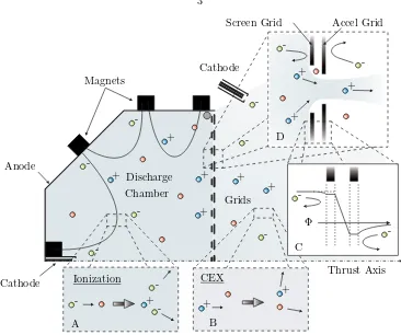
neutral atom (inset A). At the aft end of the engine is a set of extraction grids designed to allow the ions to accelerate downstream, providing thrust to the craft, while preventing the neutral propellant from drifting out of the engine (inset D).

In a two-grid system, such as that on NSTAR, the upstream (screen) grid is kept at an elevated potential with respect to the spacecraft exterior, but slightly less than that of the rest of the cham-ber; while the downstream (accel) grid is maintained at a potential less than that of the exterior (Figure 1.1, inset C). Each grid has a pattern of holes which are precisely aligned to create apertures that allow unobstructed acceleration of the ions out of the engine. These are referred to as primary ions. The purpose of the screen grid is to protect the negatively charged accel grid from attracting the accelerating ions. Electrons emitted by a neutralizing cathode downstream of the engine combine with, and neutralize, the ions, preventing the spacecraft from building up a negative charge.

The accel grid is kept at a negative potential to prevent the neutralizing electrons from accel-erating upstream into the discharge chamber. The effect of the differing potentials placed on the two grids creates a focussing effect on the ions being extracted, much like that found with an optic lens. This “ion optics” mechanism results in small ion beamlets emerging from each aperture [8]. The grid apertures and operating potentials are designed to make the effective transparency to the primary ions as high as possible while minimizing the transparency to the neutralizing electrons and neutral atoms [9].

(21)

within any specific range of angles quantified by the differential cross-section [11]. The second possible outcome is that an electron will transfer from the neutral atom to the ion in what is referred to as a charge-exchange (CEX) collision. Similar to the sole case of energy and momentum transfer, there is a charge-exchange differential cross-section associated with the probability of the CEX ion (target) scattering within any specific range of angles [12].

Wherever there are charges present, we can expect to find electromagnetic potentials and fields. Downstream of the engine grids an electromagnetic field forms due to the presence of both the charged grids as well as the moving charges in the form of neutralizing electrons, primary ions, and CEX ions. In turn, the movement of the electrons and ions is affected by this electromagnetic field [13]. Measurements made both in the lab and on operating engines have shown that there is a highly divergent population of ions at large angles from the thrust axis, which collide with surfaces far removed from direct interaction with the main exhaust. These ions are primarily slow-moving CEX ions, created by glancing charge-exchange collisions, which evolve on the electromagnetic field that has developed downstream of the thruster [14].

1.2

Modeling the CEX Process

In this work there are two types of ions which we treat. The ﬁrst type consists of the energetic ions emerging from the apertures in the form of beamlets. These are the ions that we consider to be “projectiles” in charge-exchange collisions, and we refer to them as the primary ions. The second type of ion is created from “target” atoms as a result of charge-exchange collisions. These ions begin as neutral atoms and then each lose an electron to a primary ion during collision. We refer to these newly created ions as CEX ions.

(22)

collision with the same thermal velocity that the neutral atoms had before encountering the primary ion [15, 16]. Once ionized as a result of the charge-exchange process, the CEX ions are subjected to the electric field downstream of the engine. As we will also see in Chapter 4, there is a significant radial component to the electric field — especially near the edge of the main beam of primary ions. In addition, the axial component of the electric field is directedupstream at the edge of the main beam. Under this assumption of no energy or momentum transfer, the CEX ions are completely under the influence of the electric field and are accelerated outwards in a radial direction from the beam, in addition to back towards the spacecraft [17].

While the assumption used in the current models is well founded and applicable to most of the CEX ions created, a question still remains. What happens when a CEX collision occurs during which there is also a transfer of energy? We have stated, without evidence for the moment, that the diﬀerential cross-section highly favors those collisions that transfer little to no energy. Let us assume, for argument’s sake, that for every one thousand CEX collisions involving no energy transfer there is one collision where ﬁve percent of the energy of the primary ion, 50 eV, is transfered to the neutral atom in addition to the electron transfer. Let us also assume that these collisions occur at points in space that are at an elevated potential, say 20 eV, with respect to the surface of the spacecraft.

Imagine all of the CEX ions accelerating through the electric ﬁeld and colliding with the space-craft surface that was at a potential 20 eV lower than the point where the ions were created. The one thousand ions will collide with an energy of 20 eV and the single ion initially imparted with 50 eV will collide with the surface with an energy of 70 eV. In this situation the question of which does more damage to the surface arises. Is it possible that the collision of one ion with 70 eV of energy results in more damage than the cumulative eﬀect of one thousand ions with 20 eV? The models which assume there is no energy transfer during the charge-exchange process cannot answer this question.

(23)

and momentum transfer process during charge-exchange collisions, and more speciﬁcally, a model that can predict the amount of sputtering that one would expect at any particular point around the engine due to impacts from the CEX ions.

For reasons that are dictated by elastic collision dynamics and will be made apparent in Chapter 4, models that do not account for energy or momentum transfer only require total CEX ion production rates. The production rate at any particular point in space does not depend on the direction of motion of the primary ions; the rate depends only on the total current passing through the point [13]. In contrast, inclusion of energy and momentum dynamics in a charge-exchange plume model allows the direction of the primary ions to have a direct impact on the trajectory that a CEX ion will take after the collision. Since the source of primary ions determines the trajectories of these ions, the ion source itself has inﬂuence over the behavior of the CEX ions. This implies that, if one were to change the ion source, one could potentially increase or decrease the amount of sputtering that occurs at any particular surface due to CEX ion impacts.

If we can define the ion engine grids to be the source of ions, an immediate application of a model incorporating charge-exchange collision dynamics is to the design of these grids. Any spacecraft designer concerned about sputtering of surfaces on his craft can of course take the approach of building it such that nothing of importance is anywhere near the engine. This is the simple and uninteresting solution, and due to possible limitations, such as available space, may not be a viable option. The ability to design the engine to fit with the specific craft and mission could be extremely valuable; however, we understand that the grids on an ion engine can not be redesigned with complete impunity. In the next section we will discuss restrictions on the design of ion engine grids and how this leads to the second goal of this thesis — a constrained optimization of ion engine grid shapes.

1.3

Limitations to Ion Engine Grid Design

(24)

would experience during launch before being released from the launch vehicle and inserted into its ﬁnal orbit or trajectory [18]. During this test it must be shown that the craft has the structural integrity to survive the launch. The ion engine grids, critical to the operation of the entire engine, could easily fracture if not designed carefully, and cause catastrophic failure that could endanger the success of the entire mission of the spacecraft.

For perspective, the grids on the NSTAR engine that ﬂew on Deep Space One were 30 cm in diameter, 0.38 mm (screen) and 0.51 mm (accel) thick, and separated by a scant 0.66 mm [9]. Had the launch environment proven to be too much for the grids such that they collided with each other, or simply fractured due to too much stress, the entire Deep Space One mission would have been in jeopardy. To prevent this possibility as well as to provide thermal-mechanical stability to the grids so that they wouldn’t thermally expand and come into contact with each other during operation, the NSTAR ion engine grids were spherically dished [9].

(25)

1.4

Thesis Overview

The general mathematical foundation for the work to follow is presented in Chapter 2. In Section 2.1 we derive the equations to be solved by the CEX ion model. The equations of primary importance are the CEX ion energy distribution at a specific point, and the sputtering integral. The energy distribution will quantify the number of CEX ions within any specific energy range that pass through the specified point. The sputtering integral will predict the total sputtering rate of a surface at the specified point due to collisions of the CEX ions described by the energy distribution. A brief discussion of the theory behind constrained optimization problem solving will follow in Section 2.2. Chapter 2 will introduce a series of different quantities that must be found in order to solve the equations presented. Chapter 3 will follow with the discussion of the first of these quantities — the neutral atom density field. A frequently used model for finding the density of neutral atoms as a result of diffusion through a set of holes or apertures is a modified cosine, or Lambertian, distribution. In Section 3.1 we present the foundation and reasoning behind the use of such a model and from where the modifiers, including the Clausing factor, originally come. Comparison of the modified cosine distribution, with results from computations of rarefied gas flow through two hole apertures, using the direct simulation Monte Carlo (DSMC) method, are presented in Section 3.2. Simulations of both a single aperture in an infinite plane and a pseudo-periodic aperture pattern are shown. The farfield distribution will be emphasized in Section 3.3, where we present the distributions obtained from the simulations for each aperture and determination of the equivalent Clausing factor for each. Chapter 3 concludes with a demonstration of how the results obtained can be applied for determining the density of neutral atoms at any point downstream of an ion engine grid. The final neutral atom density field obtained in this way will be compared to that obtained by using the common modified cosine distribution.

(26)

presents a model for determining the electric potential from the ion charge density. In turn, the model for determining the ion charge density is presented in Section 4.2. The method for integrating the equations of motion, the velocity Verlet algorithm, will be shown in Section 4.3. The definitions and experimental data used for evaluating the charge-exchange differential cross-section and sputter yield follow in Sections 4.4 and 4.5. The behavior exhibited by CEX ions that scatter at different angles, and correspondingly with different initial energies, are analyzed in Section 4.6. Behavior in a two-dimensional system will be examined first, which will introduce principles useful for interpreting the results from a three-dimensional system. Every scattered CEX ion is found to apply to one of four distinct cases, and the implications of each case on the measured energy flux distribution of CEX ions through a particular point are discussed. Among these four cases, the interesting discovery, that from any scattering event there are two unique possible scattering angles a CEX ion can scatter into and end up passing through the same point is discussed. A physical explanation for this phenomena is given, as well as the method used to determine the two unique scattering angles. Having by that point determined methods for finding all the required quantities laid out in Chapter 2, Section 4.7 introduces the concept of the beamlet shell by which computational integration of all quantities is facilitated. Through integration, the full CEX ion energy flux distribution and sputtering integral at any particular point can be computed. An example of the implementation of this beamlet shell into the computation of the flux distribution and the sputtering rate, for both one individual shell as well as for an entire beamlet, will be presented.

(27)

the grid is symmetric, even if it is, in fact, asymmetric due to an asymetric grid shape.

Discussion of how the structural component of the optimization problem is handled is given in Chapter 6. Section 6.1 presents the issues dealt with when working with perforated shell or plate-like structures. The results of theoretical and experimental work dealing with such structures are presented and summarized. In Section 6.2 we discuss the assumptions and limitations made in applying the knowledge gained from Section 6.1 to our specific optimization problem, where we deal with shaped shells instead of flat plates. The chapter ends in Section 6.3 with a demonstration of how we determine the effective properties for any grid; and the results from application of the finite-element software to a flat plate and the NSTAR grids.

The method by which the optimization was carried out and the results of some sample cases are presented in Chapter 7. In Section 7.1 we present the control mesh and how a paramterized limit surface is obtained from this mesh, which conforms to the grid shape under investigation. A brief description of the Matlab optimization algorithm is given in Section 7.2, where we set up our particular problem and determine the constraints on our optimization. Section 7.3 follows with results of sample optimization cases performed to demonstrate the sensitivity to diﬀerent elements of the model, as well as to determine some general trends that arise, which tend to lead to more optimal grid shapes.

(28)

Chapter 2

Mathematical Formulation of the

General Problem

(29)

2.1

Derivation of the Objective Function: Sputtering Rate

In this section we present the derivation of the expressions that model the expected sputtering rate of material from a surface due to impingement of CEX ions. In Section 2.1.1 a sputtering rate is derived based on the observation that sputtering is dependent both on the ion energy and angle of impingement. Similar expressions are derived in Section 2.1.2 for situations when the assumption of angle-independent sputtering may be suitable. Justiﬁcation for this assumption is presented.

Kinetic theory is a well established field and extensive discussions of the subject can be found in works by Jeans [19], Chapman and Cowling [20], Guggenheim [21], and Kennard [22], to name a few. The derivation presented here will begin with some fundamental concepts pertaining to kinetic theory, such as the velocity distribution function and the differential scattering cross-section. Jeans [19] and Chapman and Cowling [20] give thorough discussions of the velocity distribution function, and Guggenheim [21] gives an excellent explanation of the differential cross-section. Through ma-nipulation of the equation defining the differential cross-section and through detailed balance, we will derive an integral expression that describes the expected flux of scattered CEX ions through a specified volume of space due to collisions between primary ions and cold neutral atoms through-out the entire region downstream of an ion engine. This integral expression will be equivalent to a modified and simplified version of the Boltzmann equation which is used extensively in kinetic theory. For further discussion of the Boltzmann equation, refer to texts by Kennard [22], Chapman and Cowling [20], or Reif [23].

2.1.1

Energy- and Angle-Dependent Rate

Let the primary ions of classube deﬁned to be those ions with velocities betweenuandu+δ3_u_,

whereuˆis the unit vector in the direction of motion. By the deﬁnition of the velocity distribution function [20], fp(u), the number of primary ions of classulocated within a volumeδV located at

P(x) is

(30)

ˆ n ˆ u

δA

u

u·ˆnδt _ψ

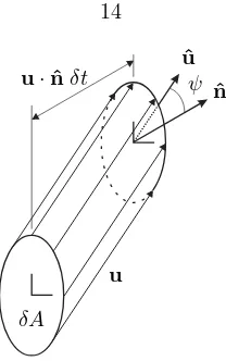
Figure 2.1: Primary ion ﬂux through a surface. Primary ions with speed uand vector of motionuˆ

pass through an area elementδAwith normal vectorˆn. In the timeδt, the ions passing through the area element sweep out a volumeδV = (u·nˆδt) δA. The angle between the vector of motion and normal vector isψ= cos−1₍_u_ˆ_·_ˆ_n_).

where

u

fp(u) d3u≡1, (2.2)

and np(x) is the total number density of primary ions within δV [24]. In the time δt, the ions of

classuthat pass through the areaδA with the normal vectorˆnsweep out the volume

δV =δx δA= (u·nˆδt) δA (2.3)

(see Figure 2.1). Therefore, the number ﬂux of ions of classupassing throughδA into the volume

δV is

δNp(x,u)

δA δt =np(x)fp(u)u·nˆδ

3_u₌_ϕ_u_ˆ_·_n_ˆ_δ3_u_, _(2.4)

where we have deﬁned the quantity

ϕ≡u np(x)fp(u). (2.5)

In the case of the NSTAR engine, the primary ions are accelerated to a speed ofu≈40 km/s [9]. In contrast, the neutral atoms diﬀusing through the grid are expected to be in thermal equilibrium with the engine walls (∼500 K), with speeds ofu0≈300 m/s [15]. The thermal velocity of the atoms

(31)

(32)

(33)

(34)

when studying a fluid. Whereas in a fluid, the definition of a streamtube precludes any mass passing into or out of the region of space bounded by the streamtube, this is not the case in our calculations. Ions scattered from a different location may very well pass through the region of space enclosed by the streamtube as we have defined here. We simply use it as the term as a convenient shorthand for the region of space swept out by ions with similar initial conditions.

Assuming the CEX ions do not undergo further collisions, Equations 2.14 and 2.15 specify the total flux (through a plane with a specific normal, ˆñ) and total density (at a target point S(˜x)) of CEX ions resulting from all possible collisions between primary ions and neutral atoms in all space. Justification for the assumption of collisionless CEX-ion trajectories will be made in Chapter 3 (Section 3.4) by application of the Beer-Lambert Law.

Sputtering is an energy-dependent process [26, 27, 28]. The momentum and energy of the particle colliding with a surface determines the total transferable momentum and energy available to surface atoms that enables them to be freed from surface binding forces. In addition to the dependence on collision energy, the angle at which a particle is incident with the sputtered surface may also determine the amount of sputtering damage done [29, 30, 31]. In order to calculate the rate at which material is removed from any surface, the energy- and angular-distribution of the colliding ions must be known. Though Equations 2.14 and 2.15 make no apparent accounting of it, the population of CEX ions at the target point will, in general, have a distribution of energies and velocity vectors. The following discussion explains how the CEX-ion population at any target point comes to have a distribution of energies, and how this distribution is obtained from Equations 2.14 and 2.15. The relationship between the ﬂux and density energy distributions will be determined.

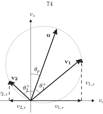
In an elastic charge exchange collision between partners of identical mass (positive xenon ion and neutral atom), conservation of energy and momentum analysis stipulates that the ion and atom initially leave the collision on trajectories separated by 90◦ in the lab frame. Both the projectile (primary ion, CEX neutral) and target atom (CEX ion) leave the collision with energies E0 _and

E+_{, respectively. Each collision exit energy is proportional to the square of the cosine of the angle,}

(35)

θ0 θ+

+

E+

E0

Figure 2.3: Dynamics of an elastic charge-exchange collision. A primary ion with energyE₀ collides with a stationary neutral atom. An electron is transferred from the atom to the primary ion creating a CEX ion and CEX neutral, respectively. The CEX ion scatters at an angle θ+ _{with an energy}

E+_{= cos}2_θ+_{. Similarly, the CEX neutral scatters at an angle}_θ0 _{with an energy}_E0_{= cos}2_θ0_.

projectile vector of motion,ˆu, i.e.,

E+ E0

= cos2θ+, and E

0

E0

= cos2θ0, (2.16)

where E₀ is the kinetic energy of the primary ion of class u(see Figure 2.3) [32]. In general, the scattering angle required to place an ion on a trajectory passing through the target point depends both on the primary-ion flux velocity vector,û, and the location of the scattering center,P(x). If the scattering occurs at a point with a potential ΦP and the target point is at a different potential

ΦS, by conservation of energy, the kinetic energy of the scattered particle must gain the diﬀerence

in potential between the two points as it arrives atS(˜x), i.e.,

ΔE+ =−ΔΦ = ΦP−ΦS. (2.17)

The combined result of each of these factors results in the expression for the energy of any particular CEX ion scattered by ions of classu, at an angle θ+ _{from a point}_P₍_x_{), at the target point}_S₍_˜_x_):

E=E0cos2θ+−ΔΦ =

mi|v|2

2 , (2.18)

where henceforth it will be understood that E refers to the kinetic energy of the CEX ion at the target locationS(˜x), andmi is the mass of the ion.

(36)

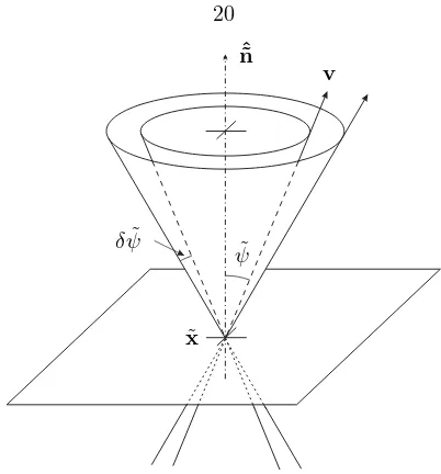
ˆ ˜ n

˜

x

˜

ψ δψ˜

v

Figure 2.4: Velocity distribution of CEX ions passing throughS(˜x). CEX ions passing throughS(˜x) with energies betweenEandE+δE (or speeds betweenvandv+δv) and at angles between ˜ψand

˜

ψ+ d ˜ψ, with respect to the plane normalˆ˜n, are classiﬁed to be of class Eψ˜.

energies of CEX ions at the target point are: (1) the diverse range of values the potential diﬀerence, ΔΦ, can have due to the variation in electric potential at all the diﬀerent possible scattering centers,

P(x), and (2) the range of primary ion energies, E₀, and scattering angles,θ+_{, required to set an}

ion on a path throughS(˜x) due to the variation in primary ion velocities,u. Later we will see that, depending on the location of the target point and the actual plume potential, the varying values of the potential diﬀerence, ΔΦ, can account for an energy spread of up to approximately 20 eV. The range of primary-ion velocities and resulting scattering angles can account for a much larger spread in energies.

Of all the CEX ions passing through S(x˜) (see Equations 2.14 and 2.15), let us deﬁne those ions passing through the target point with energies betweenE andE+δE(corresponding to speeds betweenvandv+δv) and at angles between ˜ψand ˜ψ+ d ˜ψ, with respect to the plane normalnˆ˜, to be of classEψ˜ (see Figures 2.2 & 2.4). In a manner similar to how we deﬁned the velocity distribution

function of primary ions at P(x) in Equation 2.1, let us deﬁne the angular energy distribution function of CEX ions to be such that the number of CEX ions of classEψ˜located in a volume δV˜

atS(˜x) is

(37)

(38)

(39)

(40)

Equa-With no angular dependence on the sputter yield, the sputtered ﬂux of Equation 2.26 reduces to

Υ = E_max

0

Y(E) Γ dE. (2.34)

The purpose of this work is to develop a method for solving the equations (especially Equa-tion 2.34) laid out in this chapter for any point in the region surrounding the exit of an ion engine thruster. Speciﬁcally, the following procedure will be followed. First, we must develop the ability to compute all of the individual quantities required to solve Equation 2.29. The neutral density,n₀, is dealt with in Chapter 3. Methods for computing the remaining quantities, the primary-ion ﬂux

ϕuˆ d3_u_{, diﬀerential cross-section d}_σ+_/_{dΩ, and the streamtube expansion d ˜}_A/_{dΩ, are presented}

in Chapter 4, in Sections 4.2, 4.4, and 4.7, respectively. Second, the non-directional energy ﬂux distribution (Equation 2.33) must be found, and is discussed in Section 4.7. The sputter yield is discussed in Section 4.5, which, in conjunction with the ﬂux distribution, may then be used to solve for the sputter rate from Equation 2.34. This last step is discusssed in Section 4.7.

(41)

2.2

Description of an Optimization Problem

The description here is a brief summary of the more complete discussion found in Papalambros [35]. As with any optimization problem, there are three key components required. The first is the objective function, a scalar function which defines that quantity which we wish to minimize. The second requirement is the set of any and all parameters which directly influence the value of the objective function. These parameters must completely define a configuration from which the objective function can be directly found. The third component to this problem is that of the

constraintson either the values of the parameters themselves, or on any functions of the parameters. The constraints can be divided into two distinct types: (1)equality and (2)inequalityconstraints.

Let us form the n-dimensional conﬁguration space, Π, spanned by all possible values of all the

n pre-determined parameters. Each point in this space, denoted by a vector,ξ, of specific values for each parameter, defines a specific configuration for which a unique value can be found for the objective function, Υ(ξ). Let us assume the constraints are represented by vector-valued functions of the subset of parameters,ξ, such that

a(ξ) =0 and b(ξ)≤0. (2.35)

The first constraint condition defines an (n−m)-dimensional hypersurface that is a subset of Π, on which the minimizing solution, Υ(ξ∗), must lie, wheremis the number of equality constraint conditions contained ina(ξ). The second constraint condition defines a set ofn-dimensional regions that are subsets of Π, and are bounded by the set of (n−1)-dimensional hypersurfaces defined by

b(ξ) =0.

The problem posed can be stated as follows:

minimize Υ(ξ) (2.36a)

subject to a(ξ) =0, (2.36b)

(42)

If we can assume that the Objective Function, Υ, is continuous and diﬀerentiable, a solution to the problem,ξ∗, must satisfy theKarush-Kuhn-Tuckerconditions:

a(ξ∗) =0,b(ξ∗)≤0; (2.37a)

∇Υ(ξ∗_{) +}_λT_∇_a

(ξ∗) +μT∇b(ξ∗) =0T, whereλ =0,μ≥0,μTb=0, (2.37b)

where ∇a= [∇a1,∇a2, ...,∇am]T is the Jacobian of a, and ∇ is the gradient with respect to the

parametersξ. The ﬁrst condition simply reiterates that the solution must meet all conditions deﬁned by the constraints. Some may recognize the second condition to be simply that found in the theory of Lagrange multipliers which states that the gradients of the function and the constraining surfaces must be linear combinations of each other.

While the constraints must always be met, the inequality constraints can be further subdivided into two types: (1)activeand (2)inactiveconstraints. Active inequality constraints are those which actually play a part in determining the location of the minimizing solution; the solution lies on these constraining surfaces (b(ξ∗) = 0) for, in the absence of these surfaces, the solution would be located at a point located within the volume excluded by the active constraint. Inactive equality constraints are those which could be removed from the list of constraints as they have no impact on the solution, since the minimizing solution is located neither on the constraining surface (b(ξ∗) = 0), nor within the volume excluded by the constraint (b(ξ∗)>0). In the simplest sense, the number of degrees of freedom (design parameters) is equal to the total number of parameters, n, minus the number of equality constraints, m, minus the number of active inequality constraints, s. In theory, each equality constraint and active inequality constraint could be used to eliminate one of the parameters in terms of the others until there were no constraints, and a new function to minimize,Υ, that is only dependent on them−n−pparameters left; in practice this may be impossible to do.

(43)

multipliers applied to the inequality constraints. Permitting elements of μ to be equal to zero is simply a combination of the active and inactive constraints; any zero value corresponds to an inactive constraint, which reﬂects that fact that it has no eﬀect on the solution.

These conditions arenecessary, however they areinsufficientto guarantee that Υ(ξ∗) is a local constrained minimum. In order for the pointξ∗to be a minimizing solution, the Hessian of the La-grangian must be positive-definite in the local vicinity of the solution pointξ∗, where the Lagrangian is defined to be

L(ξ,λ,μ)≡Υ(ξ) +λTa(ξ) +μTb(ξ), (2.38) and the Hessian is the gradient of the gradient with respect to the parameters ξ. This is akin to stating that any small step in any allowable direction away from the solution point results in an increase in the value of the objective function.

In this specific problem, we have created a model for which we can define a set of parameters that determine the trajectories of ions as they exit the engine and collide with neutrals. The subsequent evolution of each resulting CEX ion may result in a collision with some portion of the spacecraft and sputtering of material from the surface. It is this sputtering of sensitive areas of the spacecraft that we wish to minimize, and so defines what the Objective Function is. In Section 2.1 we derived the equations for which Chapters 3 and 4 are devoted to developing a method to solve. The end result is a model that computes the sputtering rate, per unit area, due to CEX ion collisions with a surface, based on a number of parameters chosen. It is this sputtering flux that we define to be the objective function.

(44)

Further, the constraints imposed on the proposed optimization will be those physical constraints on the shape of the grid set such that there is a high conﬁdence that the grids will survive the launch into space. While such quantities could include both the maximum tolerable stresses and displacements, we will consider only the maximum displacements in this study.

(45)

Chapter 3

Neutral Density Distribution

Determination

(46)

3.1

Rareﬁed Flow through Holes of Varying Depth

Rarefied gas flow is defined to occur when the Knudsen number is much larger than unity, i.e.,

Kn=λ/d1, whereλis the mean free path of the atoms anddis a characteristic dimension of the region through which the gas is flowing [36]. The first question to answer when determining the neutral density downstream of an ion engine is whether the state of the gas is in the rarefied regime or not. The discharge chamber of the NSTAR engine operates with a neutral xenon density of the order of 1018 _m−3 _{[9], yielding a mean free path of approximately}_λ_{= 22 cm for an atomic radius}

of 2 ˚A. The screen and accel grid thickness, separation, and hole radii are all of the order of 1 mm [9], yielding a Knudsen number much larger than unity, and placing the flow firmly in the rarefied regime.

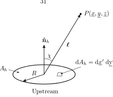
Previous models that required the determination of the neutral density around Hall thrusters [17, 37] have used a modiﬁed cosine, or Lambertian, distribution law for the particles emitted from a point located one thruster radius,Rg, behind the thruster exit:

n₀(, χ)≈W ρ₀cosχ 1− 1 1 + (Rg/)2

, (3.1)

where ρ0 is the neutral number density at the thruster exit; χ is the angle between the thruster

axis and the vector originating from the emission source and directed to the point where we wish to compute the density; is the distance between the emission source and the computation point; and

(47)

(48)

(49)

(50)

In the case of the inﬁnitely thin hole, I₀∗ =ρ₀Ahu¯0/4. We have implicitly assumed the use of a

mean velocity, ¯u₀, which results in no loss of generality, since we require that both gases flowing through the aperture and the infinitely thin hole are under the exact same conditions. By definition of the Clausing factor,

W = I0

I₀∗ = 2

π/2 0

f(χ) sinχdχ. (3.9)

Though Clausing provided integral relationships for determining the angular distribution of the flux through a hole of finite depth, statistical computation methods are typically required for more complex systems [38]. This difficulty in determining the angular distribution, f(χ), for complex geometries, such as those encountered with electric propulsion devices, has lead to the common use of the modified cosine distribution (Equation 3.5), adjusted by a Clausing-type correction factor,W

[17].

3.2

DSMC Calculation of Neutral Distribution for an NSTAR

Two-Hole Aperture

For this work, we desire to obtain an angular distribution function, f(χ), for the neutral atoms eﬀusing from the two-hole aperture created by the alignment of the ion engine grids. The holes on the NSTAR grids are patterned such that each hole is found at the vertex of an equilateral triangle (Figure 3.2). Each hole has six nearest neighbors equally spaced along a circle centered on the middle hole. The radius of this circle is equal to the hole pitch, p, and is equal to 2.22 mm for the NSTAR grids. The NSTAR screen and accel grids are 0.38 mm and 0.51 mm thick, respectively. The holes in the screen grid have a radius of 0.955 mm, and the accel grid holes have a radius of 0.57 mm. The grid separation is 0.66 mm [9].

(51)

mole-R p

Screen Accel

0.38 mm

0.66 mm

1.14 mm 0.51 mm

1.91 mm

(a)NSTAR hole spacing pattern. (b)Cross-sectional view of a single aperture.

Figure 3.2: Triangular hole pattern for NSTAR grids. Both the screen and accel grids have the same hole-to-hole pitch,p= 2.22 mm. The hole radii are R= 0.38 mm andR= 0.57 mm for the screen and accel grid, respectively.

cular ﬂow, such as those encountered when dealing with rareﬁed gases. A thorough explanation of the method can be found in [43].

3.2.1

Single Aperture in an Inﬁnite Grid

(52)

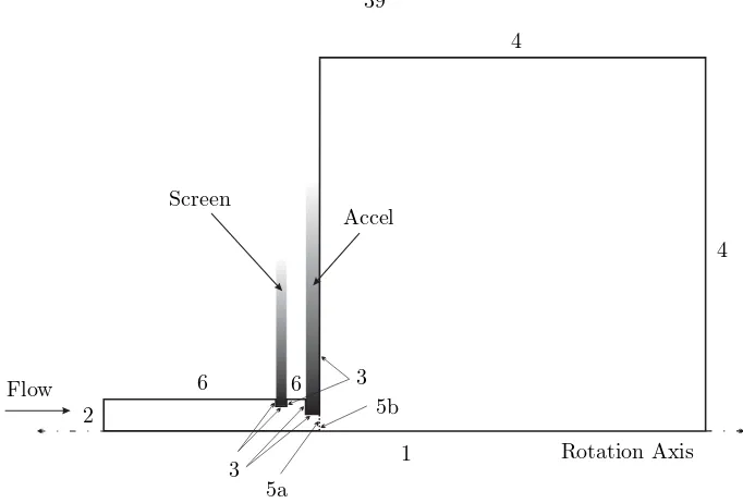
1 2

2

3

3 4

4

5a

5b Screen

Accel

Flow

Rotation Axis

Figure 3.3: Simulation domain for a single aperture in an infinite plane. Both the upstream (left of 5a) and downstream (right of 5b) domains started with zero molecules at the beginning of their respective simulation phases. The upstream flow conditions had a density of 1018cm−3, a temper-ature of 500 K, and zero mean velocity (molecules diffused in through sides 2). The positions and velocities of molecules intersecting 5a during the first phase were recorded, then the particle was removed from the domain. The recorded molecules from the first phase were used as a molecular input (at 5b) to the downstream domain in the second phase. Molecules intersecting sides 4 were removed from the simulation.

The boundary conditions for the domains used for both simulation phases follow. Boundary 1: Axis of rotation

Boundary 2: Free stream boundary

Boundary 3: Diﬀuse reﬂecting surface at a temperature of 500 K Boundary 4: Vacuum (intersecting molecules removed from domain) Boundary 5a: Vacuum (molecular output)

Boundary 5b: Molecular input

The free stream was speciﬁed to be a ﬂow of argon gas with a density of 1018_cm−3_{, a temperature}

(53)

2,400 real atoms, were in the upstream domain at any time. The position and velocity of any particle that intercepted the surface at 5a, after steady state was achieved, were recorded; the particle was then removed from the domain. Simulation continued until the states of approximately 1.2 million atoms were recorded.

During the second phase, the record from the first was used as the input atom source file for the surface at 5b. The simulation of the particles downstream was started with no atoms in the domain. For this phase, the number of atoms each simulated particle represented was reduced to nine to increase the number of simulated atoms within the domain. As the simulation proceeded the program randomly selected atoms from the input file and added them to the flow at 5b such that the total flux from this surface was the same as that through 5a during the first phase. Once a steady state was achieved, approximately 160,000 simulated molecules were in the domain at any time. Any molecule intersecting boundary 4 was removed from the simulation. The total simulation took approximately nine days on a modern desktop computer.

During both simulation phases, after a steady state had been obtained, a sample of the atom density was recorded at periodic intervals. Each sample comprised a record of the density of atoms within each cell. Over one million samples were obtained during the second phase. The average density, over these one million samples, for each domain cell was provided as output at the conclusion of the simulation. Averaging over many samples reduced any statistical ﬂuctuations that might be present at any particular time.

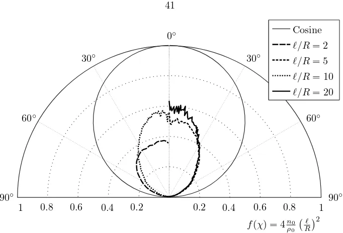
Measuring from the center of the accel grid hole (where 5b intersects the rotation axis in Fig-ure 3.3), the density at points along curves of constant radius were interpolated from the data output from the simulation. The density for various radii, as a function of the angleχmeasured from the rotation axis, is shown in Figure 3.4 in non-dimensional units. The non-dimensional density is the angular distribution function,f(χ), obtained by rearranging Equation 3.6:

f(χ) = 4n0

ρ₀

R

2

(54)

(55)

1 2

3

4 4

5a

5b 6

6 Screen

Accel

Flow

Rotation Axis

Figure 3.5: Simulation domain for a pseudo-periodic aperture pattern. Both the upstream (left of 5a) and downstream (right of 5b) domains started with zero molecules at the beginning of their respective simulation phases. The upstream flow conditions had a density of 1018cm−3, a temperature of 500 K, and zero mean velocity (molecules diffused in through sides 2). The positions and velocities of molecules intersecting 5a during the first phase were recorded, then the particle was removed from the domain. The recorded molecules from the first phase were used as a molecular input (at 5b) to the downstream domain in the second phase. Molecules intersecting sides 4 were removed from the simulation. The width of the upstream domain (distance between sides 1 and 6) is equal to one half of the NSTAR pitch,p/2 = 1.11 mm.

3.2.2

Single Aperture with a Pseudo-Periodic Hole Pattern

(56)

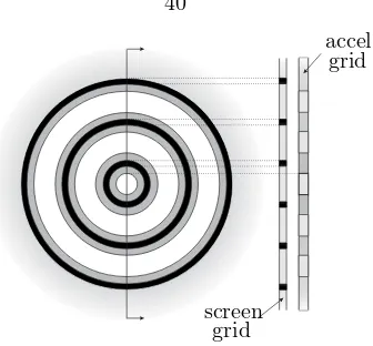
accel

screen grid

grid

Figure 3.6: Eﬀective pseudo-periodic hole pattern. The domain of Figure 3.5 models a series of concentric apertures. Though the simulation eﬀectively allows atoms to exit through the apertures surrounding the center, only those exiting through the central aperture are recorded for the purpose of populating the downstream domain (right of 5b) during the second phase of the simulation.

Boundary 1: Axis of rotation Boundary 2: Free stream boundary

Boundary 3: Diﬀuse reﬂecting surface at a temperature of 500 K Boundary 4: Vacuum (intersecting molecules removed from domain) Boundary 5a: Vacuum (Molecular output)

Boundary 5b: Molecular input

Boundary 6: Specularly reﬂecting surface

The specularly reﬂecting surfaces (Boundary 6) allow for atoms to pass from the vicinity of one hole to another. The concentric hole pattern modeled by this domain is shown in Figure 3.6. Though atoms are permitted to exit through the apertures surrounding the center, only the position and velocity of those exiting from the center aperture are recorded for the purpose of populating the downstream domain during the second simulation phase. Thus, the resulting neutral density distribution downstream of the aperture is a single-hole distribution, but the distribution of atoms upstream is inﬂuenced by the presence of other holes. The width of the upstream domain, i.e., the distance between surfaces 1 and 6, is equal to one half of the NSTAR pitch,p/2 = 1.11 mm.

(57)

(58)

(59)

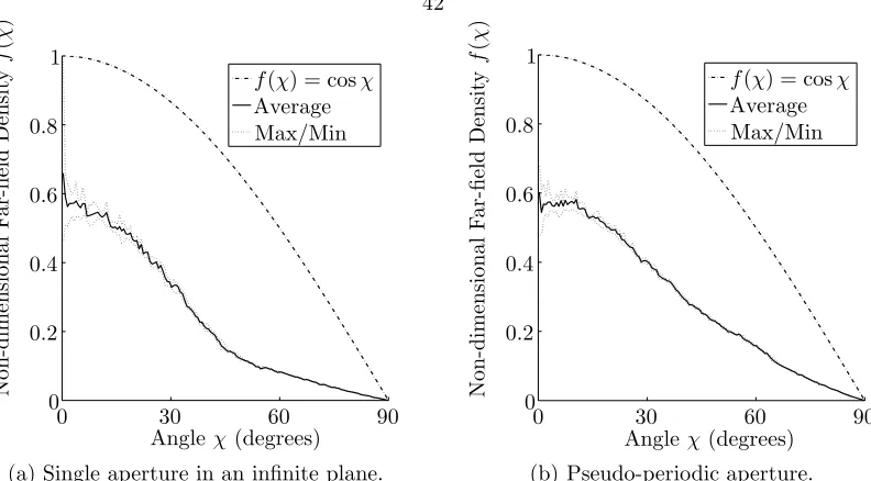
at large angles can be explained by the fact that, in the pseudo-periodic aperture, atoms that pass through the screen grid through a hole adjacent to the center hole can then pass through the accel grid through the center hole. Such atoms will have trajectories inclined at large angles with respect to the hole axis. There are some atoms present at these high angles with the single hole, since some atoms that begin travelling down the channel between the screen and accel grids can collide with a wall and be reemitted back towards the hole.

Both aperture configurations permit less flow of atoms than an infinitely thin hole, and have distributions different than the cosine. Normalizing the conditions upstream of an infinitely thin hole, such as to match the flow rate with one of the apertures, would result in a lower density along the hole axis and a higher density at large angles, compared with the density distribution of the aperture. This is demonstrated in the next section, where we compute the total neutral atom density downstream of the NSTAR grid using both the cosine and the single-aperture density distributions.

3.4

Neutral Distribution Due to Multiple Holes

(60)

3.4.1

Pseudo-Code: Calculating the Neutral Density

The following pseudo-code outlines the procedure used to determine the neutral atom density at any point. The density is computed at the desired point by superposition of the contributions from all grid holes. The code was implemented using Matlab.

1. Letxbe the location of the point at which to evaluate the density,N be the total number of holes, andRbe the accel grid hole radius.

2. Letρ0 be the neutral density inside the engine discharge chamber.

3. k= 0. 4. k=k+ 1.

5. Letyk be the coordinates of the center of holek, and ˆnk the normal vector to holek.

6. Compute the vector between holekand the evaluation point,k =x−yk.

7. Computek =k .

8. Computeχk = cos−1

−_k1k·nkˆ

.

9. If 0≤χk ≤90◦, go to step 10; otherwisen0,k= 0, go to step 11.

10. Calculate the contribution to the density from holek,

n₀,k=

ρ₀f(χk)

2 1−

1

1 + (R/k)2

. (3.12)

11. Ifk < N, go to step 4; otherwise go to step 12. 12. Sum all contributions,n0(x) =

kn0,k.

(61)

3.4.2

Neutral Density Downstream of an NSTAR Grid

The total neutral density distribution downstream of an NSTAR-shaped grid was modeled using superposition of the contributions from all grid holes. In order to prevent near-inﬁnite contributions at positions very close to the surface of the grid, the distribution contribution from each hole was calculated using the following (see Equations 3.5 and 3.6):

n₀(, χ) =ρ0f(χ)

2 1−

1

1 + (R/)2

. (3.13)

At large distances,/R1, Equation 3.13 approaches that of Equation 3.6; at a distance of 0.5 cm (∼10R), the density contributions computed from each relation diﬀer by less than 1%.

The total density was computed using both the distributions resulting from a single aperture in an infinite plane, and from an infinitely thin hole (cosine distribution). The total flux from each hole was normalized by reducing the total flux through the infinitely thin hole, i.e., f(χ) = Ws cosχ.

The procedure for computing the density at any point downstream of the grid is detailed in Section 4.4.1. The resulting density distributions, using both the single aperture and inﬁnitely thin hole, are shown in Figure 3.9.

(62)

(63)

In the derivation of the model equations in Chapter 2, we assumed that the CEX ions do not undergo further collisions once they are created from a charge-exchange collision. Now that we have estimates to the neutral density distribution around an N