J.N. Matthewsa
University of Utah, High Energy Astrophysics Institute, Department of Physics and Astronomy, Salt Lake City, UT 84112, USA
Abstract. The Telescope Array studies the properties of ultra high energy cosmic rays by measuring the extensive air showers which they induce. We do this using a variety of techniques including an array of scintillator detectors to sample the footprint of the air shower when it reaches the Earth’s surface and telescopes to measure the fluorescence and ˇCerenkov light of the air shower. From this we determine the energy spectrum and chemical composition of the primary particles. We also search for sources of cosmic rays and anisotropy. We have found evidence of a possible source of ultra high energy cosmic rays in the northern sky. The experiment and its recent measurements are discussed.
1. Introduction
The Telescope Array collaboration was forged by members of the High Resolution Fly’s Eye (HiRes) and Akeno Giant Air Shower Array (AGASA) collaborations. Its purpose is to study ultra high energy cosmic rays, their spectrum, composition, and anisotropy/sources. Additional goals included understanding the differences in the observations of HiRes and AGASA as well as the transition from galactic to extra-galactic sources. The collaboration has, over time, grown to include members from the US, Japan, Russia, South Korea, and Belgium.
The Telescope Array is located in central Utah in the US at about 39.30◦ north latitude and 112.91◦ west longitude. The high energy component of the experiment consists of 38 telescopes, (9728 PMTs) at three telescope stations overlooking an array of 507 scintillator surface detectors (SD). The SD array has an area greater than 700 km2. The main body of the Telescope Array was
complete and operational as of 2008. The layout of the TA experiment is shown in Fig.1.
We use the atmosphere as a part of our calorimeter and observe the energy deposited by the primary cosmic ray and the extensive air shower it initiates. Telescopes view the longitudinal development of the air shower as it passes through the atmosphere. The three telescope stations are located on the perimeter of the SD array (on a ∼30 km triangle) and view the sky over it. The northern telescope station has 14 telescopes, each with a 5.2 m2 mirror.
It re-utilizes telescopes from the High Resolution Fly’s Eye, HiRes-I site. The southern two stations each have 12 telescopes, with 6.8 m2 mirrors. The new telescopes at these sites use FADC electronics, while the HiRes-I telescopes are using older sample-and-hold electronics.
The cameras in the telescopes utilize 256 PMTs for pixels, each viewing about 1◦ of sky. The PMTs are hexagonal and are arranged in a 16×16 hexagonal close pack (honey-comb) array. Each site views from 3−31◦ in elevation and has full azimuthal view over the SD array.
ae-mail:[email protected]
The telescopes are looking for an amount of light similar to a 50–100 W UV light bulb, but 20–40 km away and moving at the speed of light. Due to the extreme sensitivity of the telescopes and cameras, the telescopes are only operated on clear moonless nights. This results in a duty cycle of about 10%.
The scintillator surface detector (SD) array, samples the density of air shower particles when they reach the Earth’s surface. The 507 detectors each have two layers of half-inch (1.25 cm) thick scintillator extruded with grooves in it. Wavelength shifting optical fibers are placed into the grooves. They gather the light, shift the wavelength, and guide it to two PMTs, one for each optically separated layer. Each layer samples 3 m2in area.
The scintillator surface detectors are deployed on a 1.2 km square grid. They are powered by solar panels and batteries for 24/7 continuous operations. They are self-calibrated by using the muon background and are read out by 2.4 GHz radio. Three radio towers divide the detectors among them. Each second the towers poll all of the detectors in their part of the array for signals, then a computer at the tower scans this for signs of a shower footprint. If a shower is found, then the tower requests that all data from the time period be sent back and recorded.
Each telescope station operates separately and inde-pendently from the SD array. The data from each can be analyzed separately or in conjunction with the other parts. Single telescope only data is known as “mono”, from multiple telescopes “stereo” and telescope with SD is “hybrid”. Having more information is always better since it constrains the data and reduces the uncertainties. However, one does not always have that luxury – for example the SD data set is the largest since it operates 24/7 (nearly 100% duty cycle) while the telescopes have a duty cycle of about 10% due to sun light, moon light, and weather conditions. Hence the SD only data is used where one can tolerate the slightly larger uncertainties such as in the spectrum and anisotropy measurements. Hybrid and stereo have their own places, these are required to reduce uncertainties enough to make composition measurements.
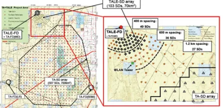
Figure 1. Layout of the Telescope Array detector site. The main array is shown on the left with a surface detector (SD) array of 507 scintillation counters surrounded by three fluorescence detector (FD) stations (MD: Middle Drum, BRM: Black Rock mesa, LR: Long Ridge) looking inward over the SD. The expanded inset on the right shows the layout of the TA Low-energy Extension (TALE). The TALE addition to Telescope Array consists of 10 new high-elevation (31◦−59◦) fluorescence telescopes located at the MD site, and an in-fill SD array of 103 counters arranged with spacings that grow with distance from the TALE FD, in order to make optimal coverage at energies below 1018eV.
2. Energy spectrum
The scintillator array has the greatest number of events. Telescope Array previously published an energy spectrum from the first four years of SD operation [1]. The energy spectrum of ultra high energy cosmic rays is now updated to include data from the first seven years of data and is shown in Fig. 2. The Telescope Array measurements are in excellent agreement with the previous measurements by the HiRes experiment. Using the first 7 years data set, the break point for the GZK cut-off [2,3] is found to be 1019.78±0.06eV. Integrating an unbroken line from 1019.78
to 1021eV, one would expect to find ∼99 events in this
range, while we actually observe 44 events. Hence, the significance of the cut-off is∼6σ.
A “dip” or “ankle” structure is also seen at 1018.70±0.02eV. The simplest explanation for the
combina-tion of spectral features is that of interaccombina-tion between extra-galactic cosmic ray protons and the cosmic microwave background radiation (CMBR) attenuating the flux via photo-pion production above the cut-off (via a resonance), and by e+e− pair production above the ankle [4]. The Telescope Array spectrum shows an apparent break at just above 1017eV consistent with the “Second
Knee” feature [5]. Another dip feature is seen just above the 1016eV, which has been previously reported by other
experiments [6,7].
When the Auger spectrum is scaled up by 10% in energy (well within the energy uncertainties of both experiments, the Auger spectrum is also in good agreement with the Telescope Array and the HiRes spectra at lower energies. However, for E>1019.3eV, the two spectra
appear to diverge. The Auger spectrum has a significantly lower cut-off energy. Understanding this discrepancy is one area of joint study between the two groups.
3. Composition
We measure the composition with the Xmax technique. That is, we measure the depth of shower maximum in the
Figure 2. The combined spectrum from the Telescope Array Collaboration, including the first 7 years data from the surface detector spectrum (upright triangles), the 7 year monocular spectrum from the Black Rock and Long Ridge fluorescence detectors (inverted triangles), the TALE fluorescence spectrum (open circles), and the TALE ˇCerenkov spectrum (open squares). The averaged spectrum combining these four measurements is shown by the black circles.
atmosphere and we use Monte Carlo models to correlate this with chemical composition of the primary cosmic ray. Protons have a smaller cross-section and interact deeper than heavier nuclei. The distribution also has more width to it. However, there is considerable overlap to the distributions, so one mostly looks at mean Xmax behavior and width behavior. These shift as a function of energy and this is called elongation.
To measure composition, one requires hybrid or stereo data in order to constrain the geometry and thereby to make a well understood measurement of Xmax, the depth of shower maximum. One advantage of stereo data is that it also provides a redundant measurement of Xmax which allows a resolution verification measurement. With hybrid, one extends the timing information in the angle vs. time plots which one uses to measure the pointing direction of the incoming cosmic ray. In addition, one gets the core location of the shower footprint on the Earth’s surface. These additional constraints tie down the geometry.
As of 2010, the two main measurements of composi-tion of ultra high energy cosmic rays came from HiRes and Auger. The HiRes experiment found a composition which was very light, consistent with protons between 1018.2eV and 1019.7eV. The HiRes data is, in fact, in quite good agreement with the QGSjet-01 proton model. The Auger experiment found that the composition was light in the lower energy range, but shifted to a heavier and heavier composition for E>∼1018eV.
The Auger surface detector is composed of thick water tanks. These have different sensitivities for electrons and muons. The Auger experiment has decided that the EPOS hadronic model does the best job of modeling its data. Unfortunately, there is a fairly wide dispersion between the various hadronic models and where they place the mean Xmax of protons, helium, nitrogen, and iron.
Figure 3. The comparison of the Telescope Array hybrid data with the QGSjet II.03 model. The top left histogram show the comparison of the Telescope Array data (black points) with the QGSjet II.03 model (blue for the proton model and red for the iron model) over all energies. The data is clearly more proton-like than iron-proton-like. This is quantified by performing a Cramer von-Mises test (CvM) which yields a p-value of 0.0024 for protons, but a p-value of 10−227 for iron. The other five panels
of the plot show the same plot, but broken up into energy bins. For all bins, including E>1019.2eV, the data clearly agrees much more closely with the protons than the iron. Even in that sub-set of data the CvM p-value for comparison to the proton model is 0.05, while it is 10−24for iron.
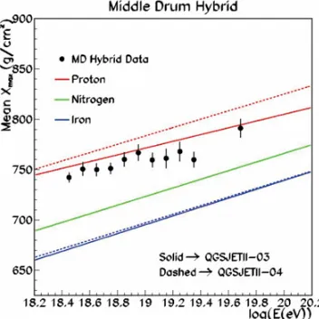
Figure 4. The Elongation Plot for the hybrid data from the Middle Drum site. The mean Xmax is plotted as a function of energy. The data is shown as the black points. The Monte Carlo results for two different hadronic models QGS-jet II.03 and QGSjet II.04 are shown for a) protons (red), b) nitrogen (green), and c) iron (blue). The data most closely resembles the QGSjet II.03 proton Monte Carlo.
to make the hybrid measurements to see if this contributed to any of the difference.
At the Telescope Array, we instituted a pattern recognition cut to verify that we were seeing both the rise and the fall of the shower development profile. With these cuts, the Xmax resolution is∼25 gm/cm2over all energies.
Figure3shows the data-Monte Carlo comparisons for the Telescope Array hybrid Xmax data with the QGSjet-II.03 model for protons and iron. In all cases, especially when one divides the set up into energy bins, the data looks much more like protons than iron.
Plotting the mean as a function of energy results in what is called an elongation plot. The elongation plot for the hybrid data from the Middle Drum site is shown in Fig. 4. As in the data-Monte Carlo comparisons for the
Figure 5. Shift plot showing how much one would have to shift Xmax in a given energy bin to make the mean Xmax of data align with the QGSjet II.03 Monte Carlo. Three examples are given for protons (red), iron (blue), and nitrogen (magenta). After each given shift, the goodness of fit is calulated and assigned an s-value. One can see that the proton Monte Carlo requires a small shift (well within uncertainties) and that the goodness of fit is also very good, though dropping a bit at the highest energies. The iron MC requires a shift of about 60 gm and even after that, the result has a very poor fit. The nitrogen MC does not fare much better than the iron MC. It requires a shift of about 40 gm and also has poor fit comparisons. The pink and blue bands show the spread due to using other hadronic models. Unfortunately, this spread is quite large.
energy slices, the data looks most like the QGSjet-II.03 proton Monte Carlo.
Another way to display this information is in what we call a shift-plot. We determine how much we would have to shift the Xmax distribution to get the best agreement between data and Monte Carlo. In Fig.5one can see that to get agreement with the proton Monte Carlo requires a shift of only a few grams, well within the measurement’s uncertainty. However, a shift of more than 60 grams is required for the iron Monte Carlo. In addition, the points on the plot are colored by their s-value, or probability of agreement in the two shapes after the shifts in mean. One can see that over all energies the proton Monte Carlo has high s-values, though dropping a bit in the highest energy bin. However, over all energies, the iron Monte Carlo shows very low s-values. The data rejects iron. The same shift plot is shown for nitrogen which requires a shift of about 40 grams and also yields very low s-values over the energy range.
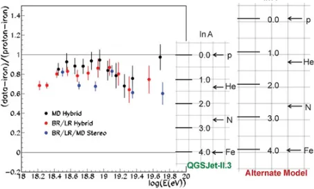
Figure 6. Summary of average XM A X from Telescope Array
fractional as the fractional position between the expectations of pure iron (lower lines at zero) and pure proton (upper line at 1.0) using the QGSjet-II.03 hadronic model. At right is the illustrative interpretation, in terms of ln A of the summary plot against QGSjet-II.03 and an alternative model where the proton rail is about 33% deeper in XM A X.
1020eV have an interaction length of hundreds of Mpc, while helium with E >1019eV has an interaction length
which rapidly falls to the 10’s of Mpc and lower. Simply, the helium can not reach us except from nearby sources.
4. Anisotropy
The Telescope Array collaboration has previously pub-lished that we have observed indications of a potential hotspot in the arrival direction of ultra high energy cosmic rays. [9] This publication used the data from the first five years of SD operations. Using the Auger criteria for their published AGN correlations, we observe 72 events with E>5.7×10¹⁹eV. These events are then over-sampled using 20◦ circles. We find that 19 of the 72 events overlap a region we call the hotspot which is centered at 146.7◦ in right ascension and 43.2◦ declination. Thus, 26% of events are in about 6% of the observable area. We expect a background of 4.5 isotropic events in this area. The Li-Ma significance of this is about 5.2σ. Taking into account that this spot could appear anywhere in the sky gives us a chance probability estimate of 3.4σ.
The hotspot is about 19◦off of the super-galactic plane, near Ursa Major. The Ursa Major super-cluster is extended more than±10◦from the super-galactic plane. Therefore, we can not rule out some sort of relationship between the hotspot and this super-cluster.
When we update the measurement by adding two additional years of data, there are 37 new events in the data set for a total of 109 events with E>5.7×10¹⁹eV. There
are 4 new events in the hotspot (3 in the 6th year and 1 in the 7th year). The expected background for this is 2.3 events. The global excess chance probability is 3.7×10⁻⁴,
which corresponds to 3.4σ, the same as for the first 5 years. A K-S test shows that the rate of arrival of events to the hotspot is consistent with the fluctuations expected from a Poisson distribution with a mean of 3.4 events/year. The rate of event arrivals is also inconsistent with chance excess from an isotropic distribution, a Poisson average of 0.9 events/year, at about the 2.6σ. One interesting thing to do is to make a full-sky map combining the Telescope Array and Pierre Auger events with E>5.7×10¹⁹eV. See
Figure 7. Full sky map combining the Telescope Array and Pierre Auger data events with E>5.7×10¹⁹eV. The events have
oversampling with a 20◦radius circle. The Telescope Array data set includes 109 events, representing the first 7 years of data collection. The Auger data set includes 157 events, representing 10 years of data. No correction was made for the energy scale difference between the Telescope Array and Pierre Auger data sets.
Fig. 7. The plot is shown in Hammer-Aitoff projection, in Equatorial coordinates. No correction was made for the energy scale difference between the Telescope Array and Pierre Auger data sets. The thin gray line just above and left of the Telescope Array (upper) hotspot is the supergalactic plane. The pre-trial significance of this is 5.2σ (post-trial chance probability of∼3.4σ). The Auger “warm spot” (lower) is located on the supergalactic plane at Centaurus-A and has a pretrial significance of ∼3.6σ. Neither the Telescope Array, nor Pierre Auger data shows any sign of excess in the direction of Virgo.
The Auger group reported correlation of their high energy, E>5.7×10¹⁹eV, events with the 472 AGNs from
the Veron catalog with Z<0.018. The Telescope Array group has looked periodically for this correlation, but have yet to find any significant correlation. The number of Telescope Array events correlating with AGNs is about 1σ greater than the background.
We have also looked for correlation with the Large Scale Structure (LSS). This is done by comparing to the matter distribution observed by the 2MASS Galaxy redshift catalog (XSCz). The sky was divided into five intensity regions, these were then compared by a Kolmagorov-Smirnov test comparing to the expected flux distribution. For events with energies, E>1018eV
and E>4×10¹⁹eV, the test can not distinguish between
the Large Scale Structure and isotropy. However, for events E>5.7×10¹⁹eV, the KS test indicated that the
data is marginally incompatible with an isotropic source distribution and it is compatible with the LSS simulation.
5. Future plans
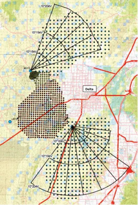
Figure 8. Map showing the Telescope Array with the high energy expansion, TA×4. The main Telescope Array with 1.2 km spacing is shown with the red points. The TALE, Telescope Array Low Energy Extension is shown as yellow points. This is a graded array with 1.2, 0.6 and 0.4 km spacing. The TA×4 expansion is shown to the NE and SE of the main Telescope Array with the dark points at 2.08 km spacing. The large blue points indicate the telescope stations. New telescopes will be added to the northern (Middle Drum) and south-eastern (Black Rock Mesa) telescope sites to view the sky over the TA×4 scintillator array expansion. The field of view of the 12 new telescopes is shown as the black fan with radii drawn to indicate the rough viewing distance for a vertical shower with energy 1018, 1019, and 1020eV. The white
space (with many red lines – roads) to the right of the main Telescope Array is the town of Delta.
in Delta, Utah and 70 more are currently being assembled in the Akeno Observatory of the University of Tokyo. The first set of scintillator detectors will be deployed early in 2017. With this enlarged Telescope Array detector, we will be able collect the equivalent of 19 current Telescope Array SD years of data by 2020. With the new data from the TA×4, we will be able to quickly verify the hotspot and to begin searching for sub-structure within the hotspot. If there are really two separated sources there, we would begin to be able to resolve this.
6. Summary
The Telescope Array has measured the energy spectrum, composition, and arrival direction of ultra high energy cosmic rays in the northern hemisphere. The low energy
is consistent with a light composition for E>1018.2eV
from both hybrid and stereo measurements. We have also reported on a hotspot near the direction of Ursa Major with a 3.4σsignificance. We need more data to verify the source and to better to resolve it. More data is needed, but more data is coming with the expansion of TA×4.
The Telescope Array experiment is supported by the Japan Society for the Promotion of Science through Grants-in-Aids for Scientific Research on Specially Promoted Research (21000002) “Extreme Phenomena in the Universe Explored by Highest Energy Cosmic Rays” and for Scientific Research (19104006), and the Inter-University Research Program of the Institute for Cosmic Ray Research; by the U.S. National Science Foundation awards 0307098, 0601915, 0649681, 0703893, 0758342, 0848320, 1069280, PHY-1069286, PHY-1404495 and PHY-1404502; by the National Research Foundation of Korea (2007-0093860, R32-10130, 2012R1A1A2008381, 2013004883); by the Russian Academy of Sciences, RFBR grants 11-02-01528a and 13-02-01311a (INR), IISN project No. 4.4502.13 and Belgian Science Policy under IUAP VII/37 (ULB). The foundations of Dr. Ezekiel R. and Edna Wattis Dumke, Willard L. Eccles and the George S. and Dolores Dore Eccles all helped with generous donations. The State of Utah supported the project through its Economic Development Board, and the University of Utah through the Office of the Vice President for Research. The experimental site became available through the cooperation of the Utah School and Institutional Trust Lands Administration (SITLA), U.S. Bureau of Land Management, and the U.S. Air Force. We also wish to thank the people and the officials of Millard County, Utah for their steadfast and warm support. We gratefully acknowledge the contributions from the technical staffs of our home institutions. An allocation of computer time from the Center for High Performance Computing at the University of Utah is gratefully acknowledged.
References
[1] T. Abu-Zayyad et al. (TA Collaboration), Astrophys. Journal Letters 768, L1 (2013)
[2] K. Greisen, Phys. Rev. Lett. 16, 222 (1966)
[3] G.T. Zatsepin and V.A. Kuz’min, JETPL 4, 78 (1966) [4] V. Berezinsky, A.Z. Gazizov, and S.I. Grigorieva,
Physics Letters B 612, 147 (2005)
[5] D.R. Bergman and J.W. Belz, J.Phys. G34, R359 (2007)
[6] W.D. Apel et al. (KASCADE-Grande Collaboration) Astropart. Phys. 36, 183 (2012)
[7] M.G. Aartsen et al. (IceCube Collaboration) Phys. Rev. D 88, 042004 (2013)
[8] R.U. Abbasi et al. (TA Collaboration), Astropart. Phys. 64, 49 (2015)
[9] R.U. Abbasi et al. (TA Collaboration), Astrophysical Journal Lett. 790, L21 (2014)