Statistical Analysis of Correlated Ordinal Data: Application to Cluster Randomization Trials

Scholarship@Western

Scholarship@Western

Electronic Thesis and Dissertation Repository

4-30-2013 12:00 AM

Statistical Analysis of Correlated Ordinal Data: Application to

Statistical Analysis of Correlated Ordinal Data: Application to

Cluster Randomization Trials

Cluster Randomization Trials

Ruochu Gao

The University of Western Ontario Supervisor

Dr. Allan Donner

The University of Western Ontario Joint Supervisor Dr. Neil Klar

The University of Western Ontario

Graduate Program in Epidemiology and Biostatistics

A thesis submitted in partial fulfillment of the requirements for the degree in Doctor of Philosophy

© Ruochu Gao 2013

Follow this and additional works at: https://ir.lib.uwo.ca/etd

Part of the Medicine and Health Sciences Commons, and the Physical Sciences and Mathematics Commons

Recommended Citation Recommended Citation

Gao, Ruochu, "Statistical Analysis of Correlated Ordinal Data: Application to Cluster Randomization Trials" (2013). Electronic Thesis and Dissertation Repository. 1696.

https://ir.lib.uwo.ca/etd/1696

This Dissertation/Thesis is brought to you for free and open access by Scholarship@Western. It has been accepted for inclusion in Electronic Thesis and Dissertation Repository by an authorized administrator of

Thesis format: Monograph

by

Ruochu Gao

Graduate Program in Epidemiology & Biostatistics

A thesis submitted in partial fulfillment of the requirements for the degree of

Doctor of Philosophy

The School of Graduate and Postdoctoral Studies The University of Western Ontario

London, Ontario, Canada

ii

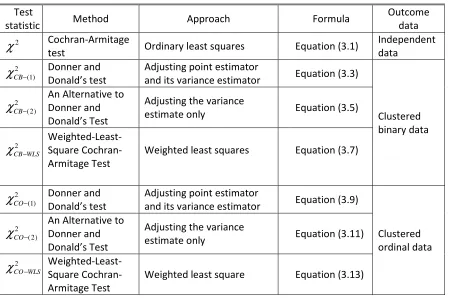
Cluster randomization trials have become increasingly popular when theoretical, ethical or practical considerations preclude the use of traditional trials that randomize individual subjects. Although some methods for analyzing clustered ordinal data have been brought to wide attention, these are less developed as compared to methods for analyzing clustered continuous or binary outcome data. The aim of this thesis is to refine existing strategies which may be applicable to clustered ordinal data as well as extensions which have been previously considered only for clustered binary responses. The approaches include adjusted Cochran-Armitage tests using an ICC estimator, and correction and modification strategies to improve the small-sample performance of the Wald test and score test in GEE for clustered ordinal data. The type I error and power for these test statistics are investigated using a simulation study.

Simulation results show that kappa-type estimators had less bias than ICC estimators when cluster sizes were fixed and small for ρ = 0.005 or ρ = 0.01. Conversely, ANOVA ICCs had relatively smaller bias in the case of variable cluster sizes. In addition, small-sample performance of GEE robust Wald tests are improved by using adjustments and corrections. The adjusted test WBC1 is recommended in terms of type I error and power.

The discussion is illustrated using data from a school-based cluster randomization trial.

iii

My deepest appreciation goes to my supervisors, Drs Allan Donner and Neil Klar. I would like to thank them for their persistent patience, warm encouragement and effective guidance while working on the thesis. Their support and insights have been invaluable. This thesis would not have been completed without their continuous help.

I am indebted to Dr. Guangyong Zou and Dr. John Koval for their excellent lectures in Biostatistics and enthusiastic help.

iv

Abstract ... ii

Acknowledgments... iii

Table of Contents ... iv

List of Tables ... ix

Chapter 1 ... 1

1 Introduction ... 1

1.1 Cluster Randomization Trials ... 1

1.2 Scales of measurements ... 2

1.3 Ordinal outcome data ... 3

1.3.1 Number of categories ... 4

1.3.2 The Television, School, and Family Smoking Prevention and Cessation Project ... 4

1.4 Analysis of Independent Ordinal Outcomes ... 6

1.4.1 Overview of Statistical Approaches ... 6

1.4.2 Scoring Ordinal Outcomes ... 8

1.5 Analysis of Clustered Ordinal Outcomes ... 9

1.5.1 Overview of Statistical Approaches ... 9

1.5.2 Estimation of the Intracluster Correlation Coefficient (ICC) ... 12

1.5.3 Non-parametric Approaches ... 13

1.5.4 Marginal Models ... 13

1.5.5 Cluster-specific Models ... 15

1.6 Testing Assumptions of Ordinal Outcome Data ... 16

v

Chapter 2 ... 19

2 Estimating Intracluster Correlation Coefficient ... 19

2.1 Introduction ... 19

2.2 Notations ... 20

2.3 Methods of Estimation ... 22

2.3.1 ANOVA method ... 23

2.3.2 Other methods ... 24

2.4 The ICC and the Measurement of Agreement ... 26

2.4.1 Introduction ... 26

2.4.2 Kappa-type ICC Estimator ... 27

2.4.3 Connections with the ANOVA ICC Estimator ... 29

2.4.4 Properties ... 31

2.5 Summary ... 36

Chapter 3 ... 39

3 Adjusted Cochran-Armitage Tests for Clustered Ordinal Outcomes ... 39

3.1 Introduction ... 39

3.2 Cochran-Armitage Test for Independent outcomes ... 41

3.3 Adjusted Cochran-Armitage test for clustered binary outcome data ... 43

3.3.1 Donner and Donald’s Test ... 43

3.3.2 An Alternative to Donner and Donald’s Test ... 47

3.3.3 Weighted Least Squares Cochran-Armitage Test ... 49

3.4 Adjusted Cochran-Armitage Test for Clustered Ordinal Outcomes ... 52

3.4.1 Extension of Donner and Donald’s Test ... 53

vi

3.5 Discussion ... 60

Chapter 4 ... 61

4 Marginal and cluster-specific models ... 61

4.1 Introduction ... 61

4.2 GEE extension of proportional odds logistic regression ... 62

4.2.1 Model formulation ... 62

4.2.2 Estimation and inference... 63

4.3 Cluster-specific extension of proportional odds logistic regression ... 67

4.3.1 Model formulation ... 67

4.3.2 Estimation and inference... 68

4.4 Relationship between Marginal and Cluster-specific Models ... 70

4.5 ICC estimation ... 72

4.5.1 ICC estimation under marginal models ... 72

4.5.2 ICC estimation in cluster-specific models ... 72

4.6 Summary ... 73

Chapter 5 ... 74

5 Adjustments to the small-sample performance of GEE ... 74

5.1 Introduction ... 74

5.2 Adjustments to the Wald test ... 76

5.2.1 Bias-corrected approaches ... 76

5.2.2 Degrees-of-freedom adjusted approaches ... 82

5.3 Adjustments to the score test ... 88

5.4 Summary ... 89

vii

6.1 Introduction ... 90

6.2 Parameters used in simulation ... 90

6.3 Generation of data ... 93

6.3.1 Cluster sizes ... 93

6.3.2 Generating clustered ordinal outcome data ... 95

6.4 Evaluation measures ... 98

6.4.1 Investigation of the ICC estimators ... 99

6.4.2 Evaluation of test statistics... 99

6.5 Computation implementation... 102

Chapter 7 ... 103

7 Simulation Results ... 103

7.1 Introduction ... 103

7.2 Estimation of Intracluster Correlation Coefficients ... 103

7.3 Adjusted Cochran-Armitage Tests ... 105

7.3.1 Type I Error rates ... 105

7.3.2 Power ... 105

7.4 Model-based Methods ... 106

7.4.1 Type I Error Rates ... 106

7.4.2 Power ... 106

7.5 Relationship between Marginal and Cluster-specific Models ... 107

Chapter 8 ... 130

8 Example: A school-based smoking prevention cluster randomization trial... 130

8.1 Introduction ... 130

viii

8.3.1 Descriptive Analyses ... 132

8.3.2 ICC Estimation... 133

8.3.3 Adjusted Cochran-Armitage Tests ... 133

8.3.4 Adjusted Model-based Tests ... 134

8.3.5 Relationship between marginal and cluster-specific models ... 135

8.4 Discussion ... 136

Chapter 9 ... 138

9 Conclusions ... 138

9.1 Summaries... 138

9.1.1 Main Findings ... 138

9.1.2 Recommendations and Discussions ... 139

9.2 Limitations and Future Research ... 140

References ... 143

Appendix A ... 156

ix

Table 1.1: Examples of recent cluster randomization trials with ordinal outcomes ... 5

Table 2.1: Analysis of variance corresponding to a completely randomized design in which clusters are assigned to each of two intervention groups ... 23

Table 2.2: Summary of the ICC estimators discussed in Chapter 2 ... 38

Table 3.1: Summary of the Cochran-Armitage trend tests in Chapter 3 ... 41

Table 3.2: Data lay-out for adjusted cochran-armitage test for clustered binary outcomes ... 44

Table 3.3: Data lay-out for adjusted Cochran-Armitage test for clustered ordinal outcomes ... 54

Table 3.4: Data lay-out for clustered ordinal outcomes in the ijth cluster ... 54

Table 5.1: Small-sample adjustments to Wald and Score tests in Chapter 5 ... 75

Table 6.1: Simulation parameters for cluster randomization simulation study ... 93

Table 6.2: Values of simulation parameters (m,m) corresponding to given (µ,λ) ... 95

Table 6.3: ICC estimators evaluated in simulation study ... 99

Table 6.4: Adjusted Cochran-Armitage test statistics evaluated in simulation ... 100

Table 6.5: Model-based test statistics evaluated in simulation study ... 101

Table 6.6: Regression coefficient estimates and their standard errors from marginal and cluster-specific models... 102

x

= 1.2, intracluster correlation

and fixed cluster size λ = 1 ... 109 Table 7.3: Properties of ICC estimators: based on 1000 simulations of trials with n

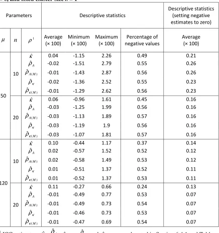
clusters of size µ per group, cumulative odds ratio θ _{= 1, intracluster correlation} ρ = 0.005, and fixed cluster sizeλ = 1 ... 110 Table 7.4: Properties of ICC estimators: based on 1000 simulations of trials with n

clusters of size µ per group, cumulative odds ratioθ _{= 1.2, intracluster correlation}ρ = 0.005, and fixed cluster sizeλ = 1 ... 111 Table 7.5: Properties of ICC estimators: based on 1000 simulations of trials with n

clusters of size µ per group, cumulative odds ratioθ _{= 1, intracluster correlation}ρ = 0.01, and fixed cluster sizeλ = 1 ... 112

Table 7.6: Properties of ICC estimators: based on 1000 simulations of trials with n

clusters of size µ per group, cumulative odds ratio θ _{= 1.2, intracluster correlation} ρ = 0.01, and fixed cluster sizeλ = 1 ... 113 Table 7.7: Properties of ICC estimators: based on 1000 simulations of trials with n

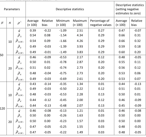
clusters of size µ per group, cumulative odds ratio θ _{= 1, intracluster correlation}ρ = 0, and variable cluster size λ = 0.8 ... 114 Table 7.8: Properties of ICC estimators: based on 1000 simulations of trials with n

clusters of size µ per group, cumulative odds ratioθ _{= 1.2, intracluster correlation}ρ = 0, and variable cluster size λ = 0.8 ... 115 Table 7.9: Properties of ICC estimators: based on 1000 simulations of trials with n

xi

= 1.2, intracluster correlation

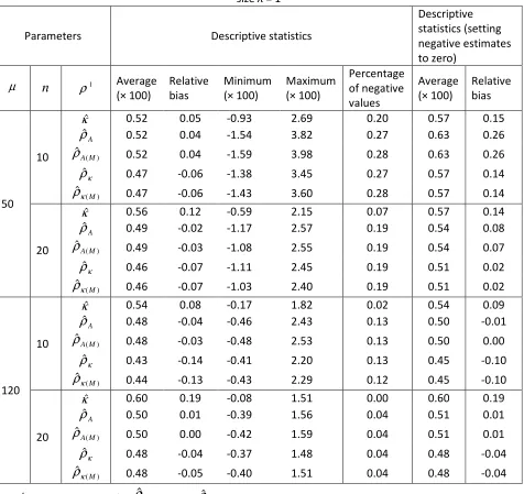
0.005, and variable cluster size λ = 0.8 ... 117 Table 7.11: Properties of ICC estimators: based on 1000 simulations of trials with n

clusters of size µ per group, cumulative odds ratioθ _{= 1, intracluster correlation}ρ = 0.01, and variable cluster sizeλ = 0.8 ... 118 Table 7.12: Properties of ICC estimators: based on 1000 simulations of trials with n

clusters of size µ per group, cumulative odds ratioθ _{= 1.2, intracluster correlation}ρ = 0.01, and variable cluster sizeλ = 0.8 ... 119 Table 7.13: Type I error rates of adjusted Cochran-Armitage test statistics1: based on 1000 simulations of trials with n clusters of size µ per group, cumulative odds ratioθ, intracluster correlationρ, and fixed cluster sizes (overly liberal or conservative type I error rates are in bold font) ... 120

Table 7.14: Type I error rates of adjusted Cochran-Armitage test statistics1: based on 1000 simulations of trials with n clusters of size µ per group, intracluster correlationρ, and variable cluster size λ = 0.8 (overly liberal or conservative type I error rates are in bold font) ... 121

Table 7.15: Power of adjusted Cochran-Armitage test statistics: based on 1000 simulations of trials with n clusters of size µ _{per group, intracluster correlation} ρ, and fixed cluster size λ = 1 ... 122 Table 7.16: Power of adjusted Cochran-Armitage test statistics: based on 1000

simulations of trials with n clusters of size µ per group, intracluster correlationρ, and variable cluster size λ = 0.8 ... 123 Table 7.17: Type I error rates of model-based test statistics: based on 1000 simulations of trials with n clusters of size µ per group, intracluster correlation ρ, and fixed cluster size λ

xii

size λ = 0.8 (overly liberal or conservative type I error rates are in bold font) ... 125 Table 7.19: Power of model-based test statistics: based on 1000 simulations of trials with

n clusters of size µ per group, intracluster correlationρ, and fixed cluster size λ = 1 .... 126 Table 7.20: Power of model-based test statistics: based on 1000 simulations of trials with

n clusters of size µ per group, intracluster correlationρ, and variable cluster size λ = 0.8 ... 127

Table 7.21: Regression Coefficient Estimates and their Standard Errors from marginal and cluster models: based on 1000 simulations of trials with n clusters of size µ per group, intracluster correlationρ, and fixed cluster size λ = 1 ... 128 Table 7.22: Regression Coefficient Estimates and their Standard Errors from marginal and cluster models: based on 1000 simulations of trials with n clusters of size µ per group, intracluster correlation ρ, and variable cluster size λ = 0.8 ... 129 Table 8.1: Descriptive statistics of school size per intervention group in the TVSFP ... 132

Table 8.2: Frequencies of three-category THKS scores per intervention group (%) ... 132

Table 8.3: Estimated ICCs for the THKS scores among students within schools ... 133

Table 8.4: Adjusted Cochran-Armitage test statistics for the effect of the TV intervention using ANOVA and kappa-type ICC estimators ... 134

Table 8.5: Test statistics for the TV intervention effect from the marginal extensions of cumulative logit model for the THKS scores (SAS procedure: PROC GENMOD) ... 135

Chapter 1

Introduction

1

1.1 Cluster Randomization Trials

When allocation of individual participants is possible, the randomized clinical trial is generally regarded as the gold standard for the evaluation of interventions in health research. Over the past two decades, random assignment at higher levels of aggregation has become increasingly popular when theoretical, ethical or practical considerations preclude the use of traditional trials that randomize individual subjects (Donner and Klar, 2000, pp. 5). Trials which assign interventions at higher levels of aggregation are referred to as cluster randomization trials. The units of randomization may be families, classrooms, worksites, hospitals or communities.

The reasons for adopting cluster randomization are various, including greater administrative efficiency and the possibility of less experimental contamination (Donner and Klar, 2000; p2-4). There is also, at times, no alternative to cluster randomization as for community intervention trials when the intervention is delivered at the community level, e.g. intervention programmes that use mass media to promote smoking cessation. Gail et al. (1992), for instance, designed the COMMIT (Community Intervention Trial for Smoking Cessation) to study public education and media campaign programmes to accelerate smoking cessation among heavy smokers and to reduce smoking prevalence. As discussed by Gail et al. (1992), these community-based interventions have the potential to affect every smoker in the community. Thus, the intervention precluded individual randomization within communities.

confidence interval for the estimated intervention effect will be too narrow and could lead to a spuriously statistically significant test result. Therefore, the correlation among responses of individuals in the same cluster must be taken into account in both the design and the statistical analysis.

A review conducted more than a decade ago (Simpson et al., 1995) found that design and analysis issues associated with cluster randomization trials were not recognized widely enough. They found that only 4 of 21 trials they reviewed accounted for between-cluster variability in sample size or power calculations, and 12 of 21 trials took account of the effect of clustering in the analysis. Although the number of published randomization trials continues to increase, Varnell et al. (2004) reported that there has been little improvement in the quality of reporting cluster randomization trials from 1998 through 2002.

Fortunately, a recent review (Eldridge et al., 2008) suggests that there has been considerable improvement in the reported design and analysis of cluster randomization trials in primary care trials. Eldridge et al. (2008) reported that 21 of 34 trials they reviewed accounted for clustering in sample size calculations, and 30 of 34 trials took account of clustering effects in analysis. However, this progress is not universal. For instance, Murray et al. (2008) reviewed 75 articles describing applications of cluster randomization trials to cancer research in 41 journals from 2002 to 2006. They reported that only 45 percent of the articles used the appropriative methods to analyze the results.

1.2 Scales of measurements

Steven (1946) defined measurement as “the assignment of numerals to objects or events according to rules”. He proposed four scales of measurement: ratio, interval, ordinal and nominal.

Donner and Klar (2000) provide examples of analyses where the study outcomes in cluster randomization trials are continuous and measured on a ratio scale. For example, change in cholesterol level (mmol/L) was the primary endpoint measured on students who participated in the Child and Adolescent Trial for Cardiovascular Health (CATCH) – a school randomized trial (Luepker et al., 1996).

Outcomes measured on an ordinal scale may be classified into ordered qualitative categories. However the interval between ordered categories is typically unknown and possibly unmeasurable for ordinal scale outcomes thus distinguishing them from interval and ratio scale measurements. An example is provided by Kim et al., (2005) in their cluster randomization trial which evaluated treatment of rheumatoid arthritis using an adjectival scale (Streiner and Norman, 2003 pp. 33-35). The outcome of interest was patient self-assessment of their attitude classified into three categories: poor, fair or good.

Data measured on a nominal scale are unordered and thus only gives identification values or labels to various categories. Objects with the same value are the same on some attribute or attributes. The values of the scale have no 'numeric' meaning in the way that one usually thinks about numbers. Cook and Demets (2008) observed that randomized trials rarely have nominal categorical outcomes with three or more levels. They noted that “an unordered categorical variable with three or more levels is usually not a suitable outcome measure because there is no clear way to decide if one treatment is superior to another''. Binary data are a special case of nominal data with only two categories. An example of binary data is provided by Murray et al. (1992) in their study to evaluate the effect of school-based interventions in reducing adolescent tobacco use. One of the outcomes was if students reported using smokeless tobacco or not.

1.3 Ordinal outcome data

1.3.1

Number of categories

Ordinal endpoints for randomized trials often use health measurement scales. One should then limit attention to scales which have had their psychometric properties validated. Even then there may be more than one possible choice of scale. The decision as to which scale should be selected as the endpoint will depend, in part, on the number of ordinal categories.

Suppose it is reasonable that the ordinal outcome measures some underlying continuous psychological construct (e.g. pain). Then selection of a more finely graded outcome should increase power to detect an intervention effect to the extent that subjects can discriminate between categories. In practice, there is likely little gain in power by increasing the number of categories beyond about five. This may reflect, in part, the difficulty people have in classifying objects or experiences into much more than seven levels (Schaeffer and Presser, 2003; Streiner and Norman, 2003, p28-29).

Decisions about the number of categories also have implications for data analysis. For example, the weighted kappa statistic varies as a function of category number (Brenner and Kliebsch, 1996).

1.3.2

The Television, School, and Family Smoking Prevention and

Cessation Project

Table 1.1: Examples of recent cluster randomization trials with ordinal outcomes

Reference Cluster Outcome Levels of outcome Number of

Levels Flay et al. 1995 school smoking intention increased, no change, or decreased 3 Marinacci et al.

2001 school frequency of condom use always, often or sometimes, never 3

Patton et al.

2006 school

antisocial behavior in the

past 6 months none, once, more than once 3

tobacco use in past month none, once to three times, more than three times 3 Glasgow et al

2005

general

practitioner patient satisfaction yes, doubtful or no 3

Byng et al. 2004 medical

practices severity of mental illness none, mild, moderate, or severe 4 Klepp et al.

1997 school

communication with AIDS

in the past month never to more than 4 times 4

McCusker et al.1992

medical

practices drug-use behavior

no injection, injection but no borrowing, borrowing but bleach always used, bleach used sometimes, bleach never used

5

Howard-Pitnet

et al. 1997 class nutritional attitude strongly agree to strongly disagree 5

Rosendal et al.

2003 physicians

classification of the patient problem

physical disease, probable physical disease, medically unexplained symptoms mental illness, no physical symptoms

5

Seligman et al.

2005 physicians physician satisfaction very dissatisfied to very satisfied 6 Watson et al.

2005 families severity of injury

minor, moderate, serious, severe, critical, or

Flay et al. (1995) report on a school-based smoking prevention programme. Seventh-grade students were randomized by school into a school-based social resistance curriculum or a television-based tobacco use prevention and cessation programme using a factorial design. Study outcomes of interest included measures of tobacco and health knowledge, coping skills and the prevalence of tobacco use. There were 7351 students who participated in the pretest assessment. These students came from 340 classrooms drawn from 47 schools.

Study outcomes included a tobacco and health knowledge scale defined as the number of correct answers to seven questions. Hedeker and Gibbons (1996) described application of a mixed effects ordinal logistic regression model to examine the effect of intervention on tobacco and health knowledge. For these analyses outcomes were grouped into quartiles given by 0-1, 2, 3 and 4-7 correct answers. These data will be used to illustrate methods of analysis for correlated ordinal outcomes. Detailed analyses are provided in Chapter 7.

1.4 Analysis of Independent Ordinal Outcomes

1.4.1

Overview of Statistical Approaches

Analytic methods for clustered ordinal outcomes are largely extensions of analytic methods for independent ordinal outcomes. Methods for analysis of independent ordinal outcome data may be classified into three approaches: non-parametric, simple linear regression and ordinal logistic regression. Moreover, attention is restricted to methods comparing two independent samples. Additionally, a distinct classification is provided by Agresti and Coull (2002) where they distinguish methods for clustered ordinal outcomes by inequality constraints. However, they noted that inequality-constrained methods are not prominent in the literature and software used for data analysis.

Another common strategy for ordinal data analysis is the assignment of scores to categories and then simply treating the scores as continuous and fitting these using linear models which assume outcomes are normally distributed. This approach has the virtue of familiarity, yielding easily interpretable, albeit potentially misleading, coefficients; however, limitations may arise from ignoring either the discrete nature or the potentially skewed distribution of ordinal data, thus violating the normality assumption. When models for continuous data are directly applied to ordinal data, a further problem is that the ceiling and floor effects of the dependent variable can result in biased estimates of the regression coefficients (McKelvey, 1975; Hedeker and Gibbons, 1994). The robustness and power of this strategy were investigated through computer simulation by Sullivan and D’Agostino (2003). Interestingly, the type I error rates obtained for tests of the effect of intervention were at the nominal level when two sample t-tests were used and when an analysis of covariance (ANCOVA) model with a common slope was fit.

The ordinal nature of the study data may be more appropriately accounted for using generalized linear models (GLM). A popular model for ordinal outcome data is the proportional odds model using cumulative logits (McCullagh, 1980; Hosmer and Lemeshow, 2000, pp. 297), which assumes identical proportionality for each logit (Agresti, 2001). This model is also called the cumulative logit model. In contrast, non-proportional odds ratio extensions of this model permit a separate effect for each logit (Peterson & Harrell, 1990; Agresti, 2001). In addition to the logit link, other link functions possible for ordinal data include the probit link and the complementary log-log link (McCullagh, 1980). These are not discussed further as they are not commonly applied to analyses of epidemiologic data.

Statistical inferences may be conducted using Wald, score or likelihood-ratio methods. The Wald test uses information from the curvature of the log-likelihood function and the distance between the parameter estimate and the null parameter value. The score test is based on the slope and curvature of the log-likelihood function only at the null parameter value. It does not require the computation of a parameter estimate. The likelihood-ratio test combines the information about the log-likelihood function at both the null value and estimated value of the parameter. Hauck and Donner (1977) showed the Wald tests for coefficients from a logistic regression model may behave in an aberrant manner in that power can decrease even as the estimated regression coefficient gets larger. This behavior of Wald tests is particularly likely when the sample size is small. They recommended that the likelihood ratio test be used instead.

These model-based tests are often equivalent, at least in special cases, to well known non-parametric test statistics. For instance, the score test from a proportional odds model for a two-group comparison is identical to the Wilcoxon rank sum test (McCullagh, 1980). However, some adjustment for these tests will be needed when applied to clustered ordinal data.

1.4.2

Scoring Ordinal Outcomes

The statistical methods which have been reviewed may be distinguished by the method used to account for the inherent order of the categories or equivalently by the choice of inequality constraint (Agrest and Coull, 2002). This is accomplished for non-parametric and parametric methods by imposing a scoring scheme to the qualitative ordered categories while ordinal logistic regression accounts for ordinality by imposing constraints on the odds ratios.

Methods of assigning scores have been described by Armitage (1955) and by Graubard and Korn (1987):

1. Scores may be linearly related to a quantitative measurement when the ordinal outcome is obtained by degrading a variable which is more finely measured, e.g. using midpoints of categories formed by grouping scores from a health measurement scale into quartiles.

2. When no natural category scores are available equally spaced scores are often selected to detect linear components of the intervention effect although rank scores may then also be used.

3. Sensitivity analysis is recommended to explore the effect of scores on study conclusions.

Furthermore, Kimeldorf et al. (1992) reviewed the statistical tests to compare ordinal outcomes from two samples and the scores adapted for each test. They further proposed an approach to obtain the minimum and maximum values of these test statistics over all possible assignments of scores. Thus if the range of the minimum and maximum values includes the critical value of the tests statistic, they suggested that one must be aware to justify the choice of scores used in the analysis.

In this thesis, I will consider the effect of score choice on validity and power of extensions of the Cochran-Armitage test which adjusts for clustering. Additionally I will compare the Cochran-Armitage test statistic to the Wilcoxon rank sum test exploring relationships between these methods.

1.5 Analysis of Clustered Ordinal Outcomes

1.5.1

Overview of Statistical Approaches

given by the design effect DE = 1+(m-1)ρ. This parameter measures the amount by which one must increase a standard variance estimate to allow for clustering, and therefore also is often referred to as the variance inflation factor. One can use design effects to adjust standard statistical approaches for clustered data at both the design and analysis stage (e.g., Donner and Donald, 1988). One advantage of this relatively simple approach is that it avoids intensive computation. Additionally, Scott and Holt (1982) derived a design effect for the variance of estimated regression coefficients from a linear regression model, while Neuhaus and Segal (1993) extended this result to logistic regression.

The unit of analysis for clustered data may be at either the cluster level or the individual level. Schools were randomly assigned to the intervention groups as part of the Child and Adolescent Trial for Cardiovascular Health (CATCH, Zucker at al, 1995). One of the secondary objectives of this trial was to evaluate the effect of training food service personnel on the dietary quality of food services (e.g., to decrease fat content). This outcome variable was collected from school lunch menus and thus the analysis was necessarily conducted at the school level. On the other hand, health outcomes analyses were conducted at the individual level. Advantages of cluster-level analyses include the possible construction of exact statistical inferences and valid tests of significance when there are small numbers of clusters; whereas individual-level analysis allows direct examination of cluster-level and individual-level predictors and provides more efficient estimates of the effect of intervention when cluster sizes are variable, assuming adjustment for effects of clustering (Donner and Klar, 2000; p80). A unique challenge for ordinal outcomes, however, is the specification of an appropriate cluster-level summary statistic. Because of this challenge we limit attention to individual level analyses.

Modeling approaches have also been extended to correlated ordinal data. As in the case of independent ordinal data, an approach for analyzing clustered ordinal data is to treat ordinal responses as continuous and then apply more familiar approaches to the clustered continuous responses. However, Hedeker and Gibbons (1994) claimed that this strategy could bias estimated regression coefficients due to the floor and ceiling effects of outcomes. Moreover, Fielding et al. (2003) compared parameter estimates obtained using multilevel linear models and multilevel ordinal models by analyzing data on educational examination grades. They reported that the magnitude and precision of fixed effect estimates were quite similar between the two models. However, random effect estimates with continuous outcomes are somewhat sensitive to the choice of score and their precision differs from that of ordinal models. These differences need to be further examined using simulation.

Extensions of generalized linear models for analysis of correlated data may be classified as population-average models (e.g., marginal model), cluster-specific models (e.g., generalized linear mixed models) or transition models. Discussions of these models for binary data include Diggle et al. (1994), Pendergast et al. (1996), and Heagerty and Zeger (2000). In addition, Agresti and Natarajan (2001) provided a comprehensive review of marginal and cluster-specific models for ordinal outcome data.

Generally, transition models focus on the dependence of a response on previously observed responses and treat them as explanatory variables of the current response. So they are always used for repeated measurement analysis. Thus transition modeling methods will not be considered in this study.

In addition, there has been considerable attention given to their limitations. Agresti and Natarajan (2001), for instance, noted maximum likelihood fitting methods require intensive computation. Other marginal modeling strategies, for instance, Dirichlet-multinomial modeling method, could reduce the required intensive computation because the number of parameters does not vary with cluster size. As an alterative, the generalized estimating equation (GEE) approach requires specification of only the first two moments but the associated robust variance estimator is biased downward when there are few clusters (e.g., Murray et al., 2004). For cluster-specific models, maximum likelihood become challenging when there are more than five random effects. In particular, the use of Gauss-Hermite quadrature approach for approximating the likelihood function will be limited (Hedeker, 2003). However, admittedly the challenge to fitting mixed effects models noted by Hedeker (2003) is of limited concern for most cluster randomization trials as then concern typically focuses on only a single between-cluster source of random variation.

1.5.2

Estimation of the Intracluster Correlation Coefficient (ICC)

1.5.2.1

Estimation for Clustered Continuous and Binary Data

Various estimators of the ICC have been reviewed in the literature (Donner, 1986; Ridout et al., 1999). There are at least three frequently used estimators of the ICC for clustered continuous and binary data. These include the one-way analysis of variance (ANOVA) estimator, the method of moments estimator and the fully parametric approach estimator. Klar (1993, p57-61) gave detailed discussions on these three methods for clustered binary outcomes.

1.5.2.2

Estimation for Clustered Ordinal Data

the ICC for clustered ordinal data by assuming that the study outcome follows a Dirichlet-multinomial distribution (Lui et al., 1999).

1.5.3

Non-parametric Approaches

Non-parametric methods occupy an important role given that they perform well without the need to make distributional assumptions. Simple adjustments to standard methods also allow them to be applied to clustered ordinal data. For example, Rosner and Grove (1999) generalized the Wilcoxon rank sum test to account for clustering by introducing four separate correlation parameters into the variance formula; Brunner and Langer (2000) extended the same test by formulating nonparametric hypotheses by means of the marginal distribution of treatment effects. Rosner et al. (2003 and 2006) generalized variance formulae for the Wilcoxon rank sum test and the Wilcoxon signed rank test that account for clustering effects.

1.5.4

Marginal Models

1.5.4.1

Maximum likelihood (ML) fitting

The likelihood function for a marginal logit model may be constructed as the multinomial joint probabilities while the marginal model refers to marginal probabilities. Thus it may involve complicated computation to fit marginal models using ML directly. One approach treats the model as a set of constraints on the cell probabilities and then maximizes the likelihood subject to these constraints (Lang and Agresti, 1994). This method is also referred as Lagrange’s method (Aitchison and Silvey, 1988; Haber, 1985; Haber and

In addition, the Dirichlet-multinomial distribution has been used to model clustered ordinal outcome data. For example, Chen and Li (1994) proposed a quasi-likelihood approach to model the association between two proportions under Dirichlet-multinomial distributions, and Lui et al. (1999) described interval estimators for the ICC and odds ratio for this model.

1.5.4.2

Generalized Estimation Equation (GEE) Approach

Lipsitz et al. (1994a) extended GEE methodology (Liang and Zeger, 1986) to marginal modeling with an ordinal response. Using a multivariate generalization of quasi-likelihood, the GEE regression estimators are consistent and the covariance estimators which use the sandwich form (e.g. sandwich estimator) are robust even with misspecification of the assumed covariance structure (Liang and Zeger, 1986). Statistical inferences may be accomplished using Wald or score test statistics. An alterative to the sandwich estimator is a model-based variance estimator, which is based on the assumed covariance structure. The sandwich estimator uses empirical evidence from the data to adjust the model-based variance in case the assumed covariance structure differs from the true one.

In spite of the wide use of GEE, small-sample performances of sandwich (robust) variance estimators for binary data have been investigated (e.g., Kauermann and Carroll,

2001; Feng and Braun, 2002). In particular, simulation studies show that the sandwich

variance estimator tends to underestimate the true variance when the number of clusters is less than 50 (e.g., Mancl and DeRouen, 2001). Consequently, the type I error for the Wald chi-square test using the sandwich estimator is inflated and the resulting confidence interval tends to be too narrow. In contrast to the liberal behaviors of robust Wald tests, Guo et al. (2005) reported that in this case the robust score test using the sandwich estimators has smaller test sizes than the nominal level.

1.5.4.3

Sandwich Estimator Corrections for Clustered Binary Data

significance testing. Lipsitz et al. (1994b) recommended using the one step GEE estimators instead of the fully iterated estimators when the binary responses are highly correlated. Additionally, resampling methods, such as the jackknife and bootstrap, have also been considered (Lipsitz et al. 1994; Sherman and le Cessie, 1997; Feng et al. 1996).

In the sandwich estimator, the unknown covariance matrix is estimated by residuals. When the number of clusters is small, the residuals tend to be negatively biased leading to underestimation of the covariance matrix. Mancl and DeRouen (2001) proposed a bias-corrected sandwich estimator by modifying the residual.

In addition, when the number of clusters is small, standard normal critical values are no larger appropriate. Kauermann and Carroll (2001) used a function of the variance of the sandwich estimator to adjust the normal distribution quantiles. Pan and Wall (2002) proposed a more general approach, adjusting the approximate t- or F-test by the variability of the sandwich estimator.

1.5.5

Cluster-specific Models

Cluster-specific models represent an extension of the generalized linear model that permits random effects as well as fixed effects (Agresti, 2002). The inclusion of random effects allows specification of the correlation between observations within a cluster.

algorithm (Booth and Hobert, 1999), and simulating the likelihood function directly by MCMC (McCulloch, 1997).

Instead of assuming a parametric distribution for the random effects, Aitkin (1999) and Santos and Berridge (2000) proposed a non-parametric mixing distribution to specify the distribution of random effects, as approximated by some mass points. Hartzel et al. (2001) combined this with the EM algorithm. Morel and Nagaraj (1993) further proposed a finite mixture distribution to model clustered categorical data.

1.6 Testing Assumptions of Ordinal Outcome Data

Armitage (1955) and Cochran (1954) derived two chi-square test statistics: one assesses the deviations from linearity of the outcome data, and the other tests the trend among binomial proportions of ordered groups. The statistic for testing the deviation from linearity could be obtained from the difference between the Pearson test statistic for association .and the trend test statistic. An analogous examination of ordinality was considered by Imrey et al. (1981) and Brant (1990) in the context of assessing assumptions of proportionality for ordinal logistic regression models.

For clustered data, Donner and Donald (1988) derived an adjusted Pearson chi-square test and an adjusted chi-square trend test. Consequently, both the Pearson and trend test statistics have been extended for clustered data. However, whether the statistic testing ordinality of clustered ordinal data could be simply obtained from the difference between those two statistics is a future topic. An analogous examination of ordinality is extending assumption assessment in ordinal regression model for independent data to clustered data. For example, Stiger et al. (1999) considered both a score test and a Wald test for assessing the assumption of proportional odds in the proportional odds model fitted with GEE.

1.7 Scope of the Thesis

clusters recruited to community intervention trials. In this thesis I limit attention to community intervention trials since these tend to have greater statistical challenges. For example, the validity of statistical inferences is often problematic when there are few large clusters.

The number of ordinal categories used in most practical applications ranges from three to five (Brenner and Kliebsch, 1996). In this thesis we restrict our attention to ordinal data with three categories. Extension of all methods to more categories is straightforward.

There are three designs that are most frequently used in cluster randomization trials: completely randomized, matched-pair and stratified. The completely randomized design is suited to trials that have a fairly large number of clusters; whereas matching or stratification is more desirable in studies with few clusters. Furthermore regression models described in this proposal may be directly extended to the stratified design. The challenge of extending the methods discussed here to pair-matched designs poses problems that are an area for future research and will not be discussed further here. The discussion will also be focused on models where there is a single binary, cluster-level covariate, i.e., trials where there is one experimental and one control group.

Among the methods reviewed above, the primary emphasis of my research is on non-parametric methods, marginal modeling, and cluster-specific modeling as applied to clustered ordinal data. For model-based methods, we limit attention to cumulative logit links.

1.8 Objectives

of existing strategies which may be applicable to clustered ordinal data as well as extensions which have been previously considered only for clustered binary responses.

Analytically, I will formulate a Cochran-Armitage test statistic for clustered ordinal outcomes data estimating an intracluster correlation coefficient for correlated ordinal data. This approach does not require complex computation or software proposed by other methods. In addition, I will develop some correction and modification strategies to improve the small-sample performance of the Wald test and score test in GEE for clustered ordinal data.

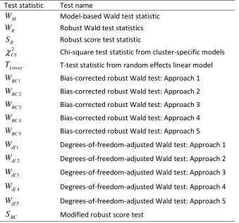
In addition to this analytic work, I will conduct simulation studies comparing the performance of model-based methods on bias and standard errors of estimators as well as type I error and statistical power. Furthermore, I will evaluate the small-sample performance of the score and Wald tests applied in GEE for clustered ordinal outcome data. To improve their performance, I will extend small-sample adjustments proposed for the sandwich variance estimators to clustered ordinal outcome data and present a comparison of their properties.

Chapter 2

Estimating Intracluster Correlation Coefficient

2

2.1 Introduction

One of the defining features of a cluster randomization trial is the similarity among responses within a cluster, which is measured by the intracluster correlation coefficient ρ. To discuss methods of analysis for clustered data, the natural starting point is the estimation of the intracluster correlation coefficient (ICC).

Various estimations of the ICC for clustered continuous and binary outcome data have been proposed, as reviewed by Donner (1986) and Ridout et al. (1999). One could extend methods for estimating the ICC for clustered continuous and binary outcomes to ordinal outcomes. For example, Lipsitz et al. (1994) extended Liang and Zeger’s (1986) GEE approach to the proportional odds model for ordinal outcome data and proposed a moment ICC estimator. Moreover, Lui et al. (1999) generalized numerous early works (Tamura and Young, 1987; Elston, 1977; Yamamoto and Tanagimoto, 1992) and derived stabilized moment estimator, the “unbiased” moment ICC estimator, and the ANOVA estimator under a Dirichlet-multinomial model.

In addition to binary outcome data, the ANOVA estimator is frequently used for clustered ordinal outcome data by assigning scores to ordered categories. For instance, Lui et al. (1999) and Lui (2002) derived interval estimators of the ICC and the odds ratio for clustered ordinal outcomes by using the ANOVA ICC estimator under Dirichlet-multinomial distribution. The virtues of using the ANOVA estimator also include that it does not require any specialized software and sophisticated numerical procedure as other model-based approaches do (e.g., the GEE procedure). Thus, these findings and favourable properties lead us to consider using the ANOVA estimator to measure the ICC for clustered ordinal outcome data in our research.

In addition, the estimation of the ICC for clustered outcomes could arise from the literature on the close relationship between measures of intracluster correlation and interobserver agreement. Fleiss and Cuzick (1979) developed a kappa-type ICC estimator for correlated binary outcome data using direct probability calculation. Ridout et al. (1999) reported that the kappa-type ICC estimator by Fleiss and Cuzick (1979) and the ANOVA estimator are two of the three most accurate ICC estimators in terms of bias and mean square errors. Moreover, Mak (1988) proposed another kappa-type ICC estimator and noted that his kappa-type ICC estimator may yield higher efficiency than the ANOVA estimator when ρis not close to zero. In this chapter we will propose a kappa-type ICC estimator for clustered ordinal outcome data.

The remainder of the chapter is organized as follows. Section 2.2 gives notations used in this thesis. Section 2.3 gives a detailed description of the ANOVA ICC estimator and then briefly introduces other ICC estimators for clustered ordinal data. In section 2.4 we propose a kappa-type ICC estimator and explore its properties and relationships with the ANOVA estimator. In section 2.5 we summary the ICC estimators presented here in a table.

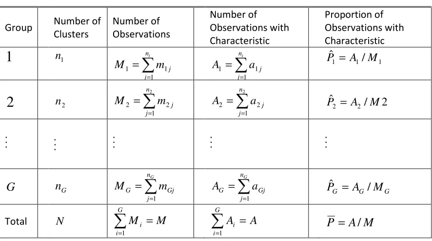
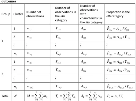
2.2 Notations

To establish notations, consider a cluster randomization trial in which ni clusters are

observation may be classified into one of K ordinal categories. Let Yijlk = 1 if the l_th

observation in the j_{th cluster from the} ith group falling into the kth category and 0 otherwise, l =1,2, …,mij, k=1,2, …,K.

We also use the following notations throughout this thesis:

∑∑

M , the total number of observations

∑

N , the total number of clusters

∑

, the total number of observations in the ith group

k ijl S

Y = , the assigned score of the kth category in which the ijlth observation falls

ijlk

Y , the indicator of outcomes where Yijlk = 1 if Yijl fall in the kth category and 0 otherwise

∑

, the number of observations in the ijth cluster falling into the kth category

∑∑

, the number of observations from the ith group in the category k

∑ ∑ ∑

= = =

=

2 1 1 1 i n j m l ijlk k i ij Y

Y , the number of observations falling in category k

∑

Y

1

/ , the numerical mean in the ij_{th cluster}

i n j m l ijl i Y n

Y i ij / 1 1

∑∑

= , the numerical mean in the ith group

N Y Y i ij n j m l ijl i / 1 1 2 1

∑∑

∑

= , the mean scores all over clusters

k

2.3 Methods of Estimation

Techniques of the ICC estimation for ordinal outcome data have been less well developed since estimations of the ICC for clustered ordinal data are not as straightforward as those for clustered continuous and binary outcome data. One of the challenges is to define a method of describing the ordinality.

One of the commonly used methods for dealing with ordinality is to assign scores to ordinal categories. For instance, the moment-based estimators Lui et al. (1999) proposed need scores corresponding to ordinal categories. The ANOVA approach may be directly applied to estimate the ICC for clustered ordinal data by imposing scores to ordered categories. Stiger et al. (1998) gave a detailed discussion on the assignment of integers when using ANOVA method to analyze ordinal data. Also, methods of scoring ordinal outcomes have been briefly introduced in section 1.4.2. In addition, one may assign weights to define the difference between ordinal distance. Cohen (1968) derived a weighted kappa statistic for ordinal data by using weights to describe the degree of disagreements among categories. Another method is to impose restrictions on odds ratios or probabilities to imply the ordinality. For example, one may derive the ICC estimators under ordinal regression models, e.g., the moment-based ICC estimator obtained from proportional odds models using GEE procedures.

The ICC estimators may be obtained by combining the above methods. For example, one has to assign both scores and weights to ordinal categories in order to obtain the weighted kappa statistic; to obtain the estimators from ordinal logistic regression models, it may be necessary to restrict odds ratios or probabilities and assign scores to categories. Additionally, there are close relationships among the three methods of imposing ordinality. For instance, Fleiss and Cohen (1973) established the equivalence of Cohen’s weighted kappa with the quadratic weight and the two-way ANOVA ICC estimator.

2.3.1

ANOVA method

Let Yijl denotes the ordinal score assigned to the ijlth observation. Consider a nested

analysis of variance model given by Y_ijl =µ+α_i +γ_ij +ε_ijl. Random cluster effects, denoted by γij, are assumed to be normally distributed with mean 0 and variance

2 c

σ , i.e.

ij

γ ~N(0,σc2). We similarly assume the error terms εijl~ (0, ) 2 e

N σ . The ICC, ρ, may be interpreted as “the proportion of overall variation in response that can be accounted for by the between-cluster variation” (Donner and Klar, 2000, pp.8), i.e.,

2 2 2 e c c

σ

σ

σ

ρ

The corresponding ANOVA table, which may be used to test the significance of the treatment effect, is shown in Table 2.1.

Table 2.1: Analysis of variance corresponding to a completely randomized design in

which clusters are assigned to each of two intervention groups

Degrees of freedom Sum of squares (SS) Mean square (MS)

Group 1 SSG MSG

Clusters

∑

= − 2 1 ) 1 ( i i

n SSC MSC

Errors

∑

= − 2 1 i i n

M SSE MSE

Total _{M −1} SST

Here MSC and MSE are the between-cluster and within-cluster mean squares respectively, given by

∑∑

∑

∑ ∑∑

∑

Then the estimated ANOVA estimator ρ_A could be written as MSE m MSC MSE MSC A ) 1 ( ˆ 0 − + − =

ρ (2.1)

where 2 2 1 2 1 1 2 0 − − =

∑

∑∑

2.3.2

Other methods

In addition to the ANOVA approach, the ICCs for cluster ordinal outcome data are often estimated by using model-based approaches. For instance, Lipsitz et al. (1994) proposed a moment-based approach to estimate ρ using generalized estimating equations (GEE) in proportional odds models. Let A_ijl be a diagonal matrix with the binary variances on the main diagonal, i.e.,

)}] ˆ 1 ( ˆ ),.... ˆ 1 ( ˆ [{ ˆ , 1 , , 1 , 1

1l ijl ijK l ijK l ij

ijl Diag P P P P

A = − ₋ − ₋

and the residual matrix

] ˆ [ ˆ ˆ 2 1 ijl ijl ijl

ijl A Y P

e = − − .

Here Pˆijkl =1 if Yijl =k and 0 otherwise, and Pˆijl =[Pˆij1l,Pˆij2l,...,Pˆij(K−1)l]'. Under a simple

case of an exchangeable correlation structure, Lipsitz et al. (1994) derived

3 )] 1 ( 2 1 [ ' ˆ ˆ ˆ 2 1 1 2 1 1 − − =

∑∑

∑∑∑

ij ij i n j i n j t s

where eˆ is estimated by substituting in ijl Aˆ and ijl Pˆ from a previous step of the Fisher ijl

scoring algorithm. We will further introduce the GEE approach in Chapter 4.

The ICC estimators may also be obtained by assuming a Dirichlet-multinomial model, e.g., a moment-based ICC estimator ρˆ by Lui et al. (1999). Consider _M n clusters are drawn from one single population and there are mj observations in the jth cluster. Let the

moment proportion estimator be

∑

∑∑

where 1(Yjl,Sk)=1 if Yjl = Sk, and 1(Yjl,Sk)=0, otherwise. Then the stabilized moment

ICC estimator is given by

where ϕ _{is a shrinkage constant.}

In addition to moment-based estimators, the ICC could also be estimated by using the MLE approach under dirichlet-multinomial models (Narayanan, 1991; Chuang and Cox, 1985; Paul et al. 2005). However, numerous authors (Tamura and Young, 1986; Tamura and Young, 1987; Yamamoto and Yanagimoto, 1992) noted that the MLE estimator generally underperforms the ANOVA and moment estimators for clustered binary outcome data with respect to the bias.

Additionally, one could derive the ICC estimator from the full likelihood function in a multivariate Plackett model (Molenberghs and Lesaffre, 1994). However, this approach

requires sophisticated numerical procedures and it is difficult to implement in practice.

2.4 The ICC and the Measurement of Agreement

2.4.1

Introduction

The kappa statistic was developed to estimate interrater agreement for categorical outcomes, where interest focuses on the similarity among ratings obtained on the same subject. Scott (1955) proposed a chance-corrected measure of agreement between two raters by assuming that the marginal distribution of proportions over categories is equal for all raters. This index is often referred as Scott’s π. Furthermore, Cohen (1960) extended Scott’s π _{under the assumption of independent and potentially different}

marginal distribution of proportions for each rater. This statistic has come to be known as Cohen’s kappa. In this study, we restrict our interests to Scott’s πand Cohen’s kappa. For other agreement measurements one could refer to the review by Banerjee et al. (1999).

Cohen (1968) generalized his kappa statistic to a weighted kappa by quantifying the severity of disagreement among ordinal categories. The most commonly used weights are “linear weights” and “quadratic weights” (Fleiss and Cohen, 1973). Furthermore, the weighted kappa statistic using quadratic weights is identical to the ICC estimator derived from a two-way ANOVA under the assumption that the subjects and the two rates are random samples from a universe of subjects and raters, respectively. As such, the relationship between kappa statistics and the ICC estimators has been built.

However, it is not appropriate to apply Cohen’s weighted kappa to estimate the ICC in cluster randomization trials because there is rarely a natural order among cluster members. For instance, the jth subject from the ith cluster is a different individual in each cluster. Thus it is not possible to estimate separate marginal distributions for each rater. As an alternative, Scott’s π _{assumes that the same marginal distribution of proportions for}

Note that both Scott’s π _{and Cohen’s kappa are derived from one single population, while}

the ICC estimates discussed here are from cluster randomization trials where there is one treatment group and one control group. As such one of challenges is to extend kappa statistics to two populations.

In next section, we propose a kappa-type ICC estimator for clustered ordinal data, denoted as ρˆ . In particular, we extend Scott’s _κ π _{statistic by using Abraira and De}

Vargas’s (1999) approach. Generally there are three improvements in the new kappa-type ICC estimator compared with Scott’sπ: one is that weights are used to define the distance between ordinal categories; the second is that it suits well for variable cluster sizes by using pairwise agreement; and the third is that it allows treatment effects.

2.4.2

Kappa-type ICC Estimator

Scott’s π _{was originally derived to measure agreement between two raters for}

multinomial outcomes. Let pk_• denotes the proportion of subjects placed in the kth

category by the first rater, p•k denotes the proportion of subjects placed in the kth

category by the second rater, and p_k the proportion of the entire subjects falling in the

kth category. Then, the kappa statistic proposed by Scott (1955) is defined as

e e o

p p p

− − =

1

π . (2.2)

Here

∑

=

=

K k

kk o p

p

1

denotes the proportion of observed agreement and

∑

=

• • _

  



 +

=

K k

k k e

p p p

1

2

2

To extend Scott’s π _{(1955) to clustered ordinal outcomes from trials where there is one}

treatment group and one control group, it is necessary to calculate P_o and P_e for each group separately. Let w_gh be the weight corresponding to the agreement between category g and h (g,h =1,2,...,K), with the conditions:

1

0≤w_gh < for g =hand w_gh =1forg≠h.

For the jth cluster from the ith group, the number of weighted agreements is:

∑∑

∑

ij w Y Y w Y Y

NA 1 1 ) 1 ( 2 1 ,

and the number of possible pairs for the ijth cluster is:

) 1 ( 2 1 − ij ij m m .

Then the estimated proportion of weighted agreement for the jth cluster in the ith group is given by: ) 1 ( 2 1 ) 1 ( 2 1 1 1 − + −

∑

∑∑

= = >

ij ij K k K g K g h ijh ijg gh ijk ijk kk m m Y Y w Y Y w .

Consequently the average observed weighted proportion of agreement for the ith group is given by

∑

∑

∑∑

=

= = >

− + − = i n j ij ij K k K g K g h ijh ijg gh ijk ijk kk i io m m Y Y w Y Y w n P 1 1 1 ) 1 ( 2 1 ) 1 ( 2 1 1

ˆ _(2.3).

) 1 ( 2 1 ) 1 ( 2 1

ˆ 1 1

− + − =

∑∑

∑

P . (2.4)`

Thus the resulting kappa-type ICC estimator for the ith group is

ie ie io i p p p ˆ 1 ˆ ˆ ˆ − − = κ ρ .

To combine kappa-type ICC estimates of the two groups, Fleiss (1980, pp. 220-222) suggested an overall value

) ˆ 1 ( ˆ ˆ ˆ ˆ 2 1 2 1 2 1 2 1 2 1 ie i ie i io i i i i i i P P P w w − − = =

∑

∑

∑

∑

∑

ρ

ρ

where the weight w_i =1−Pˆ_ie.

Therefore the kappa-type ICC estimator for clustered ordinal outcomes is calculated with equation (2.5), using equation (2.3) and (2.4).

2.4.3

Connections with the ANOVA ICC Estimator

Assuming one single population, Fleiss and Cohen (1973) reported the identity between the ANOVA ICC estimator and the weighted kappa when there are only two observations in each cluster, using the quadratic weight

2 2 ) 1 ( ) ( 1 − − − = K h g

wgh . (2.6)

In previous sections we already derived the ICC estimatorρˆ_{κ and} ρˆ assuming the trials _A where there is one treatment group and one control group,. Here we explore the relationship between these two statistics.

Substituting wgh into equation (2.3) and (2.4), Pˆio and Pˆie may be rewritten as

∑

∑

j i ij m l ij ij ijl io K m n Y m Y P 1 2 1 2 ) 1 )( 1 ( ) ( 2 1 ˆ and 2 1 1 2 2 ) 1 )( 1 ( 2 2 1 ˆ − − − − =

∑∑

Thus the kappa-type ICC estimator in Equation (2.5) could be written as

∑

∑∑

∑∑

∑

j i ij m l ij ij ijl M Y M Y m n Y m Y i ij i ij κ

ρ . (2.7)

In order to compare ρˆ in (2.7) with _κ ρˆ in (2.1), we restrict ourselves to a balanced _A cluster randomization trial (i.e.,m_ij =mand n_i =n). Thus Pˆ_io and Pˆ_ie reduce to

n K m Y m Y P n j m l n j ij ijl io 2

1 1 1

2 1 1 2 2 ) 1 )( 1 ( ) ( 2 1 − − − − =

∑∑

respectively. Therefore the kappa-type ICC estimator in equation (2.7) reduces to

n MSE m MSC MSE MSC / 1 1 ) 1 ( ˆ − − + − = κ

ρ . (2.8)

The ANOVA ICC estimator in equation (2.1) reduces to

MSE m MSC MSE MSC A ) 1 ( ˆ − + − =

ρ . (2.9)

Thus the two estimators are asymptotically equivalent as the number of clusters becomes large in a balanced trial. This result parallels Fleiss (1981, pp.226-227) and Fleiss and Cohen (1973)’s conclusions.

2.4.4

Properties

2.4.4.1

Reduction to Scott’s

π

Scott’s π _{was originally derived to measure agreement between two raters and assumes}

that all disagreements among two different categories are equal. To reduce ρ_κ to Scott’s

π _{we have to extend the original Scott’s} π _{to allow the treatment effect first. We also need}

to limit our attention to the trials where there are two observations in a cluster (i.e., 2

=

ij

m ) and the outcomes have two categories (K =2) only. Thus the weight wgh in ρˆκ

is equal to 1 when g =h and 0 otherwise.

For the ith group, the proportion of observed agreement in Scott’s π _is:

∑

io Y Y

n P 1 2 2 1 ) ( 4 1 ˆ