Performance assessment of wireless Two Way Relay Channel systems

(1)

Scholarship@Western

Electronic Thesis and Dissertation Repository

12-18-2013 12:00 AM

Performance assessment of wireless Two Way Relay Channel

systems

Siramack Ghadimi

The University of Western Ontario

Graduate Program in Electrical and Computer Engineering

A thesis submitted in partial fulfillment of the requirements for the degree in Doctor of Philosophy

Follow this and additional works at: https://ir.lib.uwo.ca/etd

Part of the Other Electrical and Computer Engineering Commons

Recommended Citation Recommended Citation

Ghadimi, Siramack, "Performance assessment of wireless Two Way Relay Channel systems" (2013). Electronic Thesis and Dissertation Repository. 1845.

https://ir.lib.uwo.ca/etd/1845

This Dissertation/Thesis is brought to you for free and open access by Scholarship@Western. It has been accepted for inclusion in Electronic Thesis and Dissertation Repository by an authorized administrator of

(2)

Way Relay Channel systems

(Thesis format: Monograph)

by

Siamack Ghadimi

Graduate Program in

Engineering Science

Electrical and Computer Engineering

A thesis submitted in partial fulfillment of the requirements for the degree of

Doctor of Philosophy

School of Graduate and Postdoctoral Studies Western University

London, Ontario, Canada

c

(3)

The objective of this thesis is theoretical investigations and numerical simulations of Two Way Relay Channel (TWRC) systems, particularly in an impulsive noise environment. Special attention is given to investigation of a TWRC system based on polarized antennas.

The first part of the thesis focuses on modeling of impulsive noise and the effect of impulsive noise on TWRC systems. The study was conducted by simulating the wireless TWRC models in the presence of impulsive noise. The bit error probability performance of the channel data was compared and at last their results are shown by graphs.

The study has been further extended to multi antenna TWRC systems. Simulation analysis of multi antenna TWRC systems in an impulsive noise environment was conducted by using a MISO Alamouti scheme and a MIMO system.

The second part of the thesis dedicated to investigation of TWRC polarization sys-tems. A new TWRC scheme based on polarized antennas has been proposed and simulated. By polarization we are able to achieve higher spectral efficiency through the use of spatial multiplexing, and improve the reliability by spatial diversity. A new network topology based on TWRC polarization systems proposed. It is well suited to mitigate effect of delay in a communication system, particularly for high priority data transmission, or increase reliability of a communication system by re-dundant transmission.

(4)

I would like to thank the department of Electrical and Computer Engineering at Western University. I am grateful to Doug Campbell for his thoughtful editing of my thesis.

(5)

Abstract . . . ii

Acknowledgements . . . iii

Table of Contents . . . iv

List of Tables . . . vi

List of Figures . . . vii

Acronyms . . . ix

1 Introduction . . . 1

I

Impulsive noise and wireless Two Way Relay Channel

sys-tem

6

2 Impulsive noise . . . 7

2.1 Introduction . . . 7

2.1.1 Literature review . . . 7

2.2 Characteristic of Impulsive noise . . . 10

2.2.1 Impulsive noise channel models for wireless system . . . 11

2.3 Conclusions . . . 14

3 Wireless Two Way Relay Channel system . . . 15

3.2 Network coding . . . 15

3.3 System model . . . 17

3.3.1 Error probability analysis . . . 19

3.4 Simulations and results . . . 23

3.4.1 TWRC vs. AF: . . . 23

3.4.2 BEP as function of SNR . . . 25

3.4.3 BEP as function of SIR . . . 27

3.4.4 BEP as function of SNR and SIR . . . 29

(6)

3.4.6 Adaptive Coding and Modulation . . . 31

4 Multi antennas in a wireless TWRC system . . . 39

4.2 System model of Multiple-Input and Single-Output TWRC . . . 39

4.2.1 Error probability analysis . . . 43

4.2.2 Simulations and results . . . 50

4.3 System model of Multiple-Input and Multiple-Output TWRC . . . . 53

II

Polarization

56

5 Polarized antennas in a wireless TWRC system . . . 57

5.2 Polarized Antenna Network Coding (PANC) and full duplex PANC . 57 5.3 System model . . . 60

5.3.1 Full duplex PANC error probability analysis . . . 67

5.4 TWRC polarization diversity . . . 80

5.5 Polarized Multicast Two Way Relay Channel (PM-TWRC) . . . 84

5.5.1 Polarized Multi Path TWRC (PMP-TWRC) . . . 85

6 Conclusions and future work . . . 87

Curriculum Vitae . . . 99

(7)

3.1 Case study of constellations types . . . 37 4.1 Values of ¯αm,n . . . 48

(8)

1.1 Noise and interference in a wireless TWRC system . . . 3

1.2 Jamming in a wireless TWRC system . . . 4

2.1 Character of Impulsive noise . . . 10

2.2 Gaussian and impulsive noise channel . . . 12

3.1 Network coding. . . 16

3.2 System Model for a Two Way Relay Channel . . . 17

3.3 Constellation of received signal at the relay node . . . 20

3.4 TWRC vs. AF relay system . . . 24

3.5 TWRC system while SIR=5 dB . . . 26

3.6 TWRC system while SIR=10 dB. . . 26

3.7 TWRC system while SIR=15 dB. . . 26

3.8 TWRC system varying SIR while SNR = 15 dB . . . 27

3.9 TWRC system while SNR=5 dB . . . 28

3.12 TWRC system varying SIR and SNR while p= 0.5 . . . 29

3.13 TWRC system with the Viterbi decoding . . . 30

3.14 An asymmetric TWRC system . . . 31

3.15 Constatation at relay for asymmetric TWRC BPSK and QPSK modulation 32 3.16 Asymmetric modulation of TWRC . . . 33

3.17 Asymmetric modulation of TWRC when|h1|=|h2| . . . 34

3.18 Optimal decision decoding algorithm (ODDA) for an asymmetric TWRC . 36 3.19 Case study of constellation types for an asymmetric TWRC . . . 37

4.1 A MISO TWRC system . . . 40

4.2 Upper and lower bounds when p = 0 and SIR = 10 dB . . . 50

4.3 Upper and lower bounds when p = 1 and SIR = 10 dB . . . 50

4.4 Upper and lower bounds when p = 0 and SNR = 5 dB . . . 51

4.5 Upper and lower bounds when p = 1 and SNR = 5 dB . . . 51

4.6 Performance comparison of different systems, SIR = 10 dB . . . 52

4.7 A MIMO TWRC system . . . 53

4.8 MIMO TWRC system vs. MISO TWRC system . . . 55

(9)

5.2 Network coding as function of time . . . 59

5.3 Polarized wave and scatter . . . 61

5.4 Geometry for the two-ray propagation model . . . 64

5.5 A cross-polarized channel . . . 66

5.6 System model for a wireless TWRC full duplex PANC. . . 67

5.7 Cross-polarized system vs. full duplex system . . . 75

5.8 Bit error probability as a function of SNR for different K-factor for SNR = 10 dB . . . 77

5.9 Bit error probability as a function of K-factor . . . 78

5.10 Polarization rotation angle . . . 79

5.11 CDF function of XPD . . . 80

5.12 XPD function of antenna rotation angle . . . 80

5.13 Comparison of MIMO cross-polarized antenna TWRC with MIMO TWRC scenarios, k=0 . . . 82

5.14 Comparison of cross-polarized TWRC with MIMO 2X2 TWRC, k=0 . . . 83

5.15 Unicast system vs. multicast system . . . 85

(10)

ACM Adaptive Coding and Modulation

AF Amplify and Forward

AM Asymmetric Modulation

ANC Analogue Network Coding

AWGN Additive White Gaussian Noise

BC Broadcast Channel

BEP Bit Error Probability

CF Characteristic Function

CSI Channel State Information

DNC Digital Network Coding

LOS Line Of Sight

MAC Multiple Access Channel

MIMO Multiple-Input and Multiple-Output

MISO Multiple-Input and Single-Output

ML Maximum Likelihood

NC Network Coding

NLOS Non Line Of Sight

PANC Polarized Antenna Network Coding

PDF Probability Density Function

PLC Power Line Communication

SEP Symbol Error Probability

SIMO Single-Input and Multiple-Output

SIR Signal-to-Impulsive-noise Ratio

SNR Signal-to-Noise Ratio

TWRC Two Way Relay Channel

XPD Channel cross-Polarziation Discrimination

(11)

Chapter 1 Introduction

The future demands calling for more robust and reliable communication systems, and demanding higher spectral efficiency, network bandwidth and capacity, lower energy consumption, and higher mobility.

To achieve these requirements, we need to have a robust wireless communication systems which should work in a dense Electro Magnetic (EM) environment. Two way communication systems appear a logical choice to satisfy these demands. Generally, the two most fundamental requirements that need to be considered for a two way communication system are the throughput of the channel, often called the speed or bandwidth, and the latency of the channel, or delay. Secondary, but important, considerations are reliability and security.

The fundamental goals of the two way communication system for the future de-mands according to the following principles can be defined as:

1. Have a full two-way real-time digital communication with high throughput or capacity for all kinds of information between all participants in the smart cities.

2. Have low delay.

3. Be able to adapt to any kind of architecture and cover the entire length and breadth of all types of communication scenarios.

(12)

5. Be stable and reliable against failures, noise, interference, and perform contin-uous self-assessments to detect and analyze matters.

6. Be robust, self-configuring, self-healing, self-upgrading and support future technology. Hence have capability to adapt to any changes in future topology without requiring termination of data transmission.

7. Be secure.

8. Be easy to install (plug-and-play) and cost effective to maintain.

Studies have shown there exist different ways of propagating and transmitting man-made noise1 through wireless communication systems. One of the most common ways is Electro Magnetic Interference (EMI) generated by an antenna.

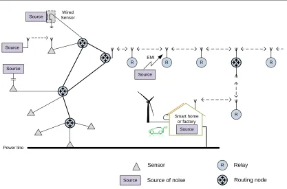
The wireless systems are subjected to interference from any electromagnetic sources, and the signal strength is greatly reduced by many materials. The presence of items such as microwave ovens, DECT phones, electrical doors, elevators, remote-control toys, machinery, electrical terrain, and many other things in the local environment will dramatically reduce the throughput and reliability of the system, see Figure 1.1. In a Two Way Relay Channel (TWRC) system [5], network coding can improve the system throughput by %100 [6].

The outage of the communication system for example jamming2, failure, natural catastrophes, attacks, etc. will directly impact the application utilizing the commu-nication system.

(13)

Routing node Sensor

Wired Sensor

Power line

R R

R

R R

Smart home or factory

R

Relay

Source of noise Source

Source

Source Source Source

Source

EMI

Figure 1.1: Noise and interference in a wireless TWRC system

The TWRC system however, will be able to continue functioning if some node(s) or some communication channel(s) fail(s), because a relay algorithm will detect, raise an alarm and choose to send signals through other available path(s), known as ‘surviving path(s)’ or ‘node(s)’, Figure 1.2.

In the case of jamming, there are other ways to prevent jamming in the wireless system such as Spread-Spectrum methods3 i.e. Direct Sequence Spread Spectrum

(14)

(DSSS)4 technique [7], Frequency Hopping (FH)5 technique, and Code Division Multiple Access (CDMA)6 technique, [8], [9], [10].

R

D Jammer

Path

A

P ath

B

R

R R

Relay R

Source

Destination

S

Physical outage

Figure 1.2: Jamming in a wireless TWRC system

The wireless system discussed until now leads to an analysis of the gaps in research related to TWRC system in the following Chapters.

The major contributions from this thesis are:

Theoretical and performance analysis of a single antenna and multiple antennas TWRC system in an impulsive noise environment.

4. In DSSS, the data is multiplied with a pseudo-noise (PN) sequence to create a longer sequence. Since the PN sequence is like noise, it is inherently wideband and, as a result, it spreads the spectrum of the data sequence too, to create a noise like sequence. Because the sequence is spread over a large band, it is less prone to interference, while it has noise-like character, which makes it difficult to detect.

5. In FH, when a nod detect attacks on the current frequency, it will jump to next available frequency. Or hop over multiple frequencies together regardless of the presence of attackers.

(15)

A new algorithm called Optimal Decision Decoding Algorithm (ODDA) for an asymmetric TWRC system.

A new TWRC scheme based on polarized antennas.

Diversity polarization for a polarized antennas TWRC system.

(16)

Part I

Impulsive noise and wireless Two

(17)

Chapter 2 Impulsive noise

2.1 Introduction

Implementation of wireless TWRC system depends on the efficiency and reliability of channel capabilities. The measurements [11] have shown that in the real world background noise e.g. impulsive noise, has a direct impact on channel quality and capacity.

Most wireless communication systems are designed for voice, video, and internet data transmission and they are tolerant to errors caused by impulsive noise. This kind of error is not tolerable for sensitive data communication such as industrial control data. Thus impulsive noise channel models for wireless systems are impor-tant in determining the error rate for the design of a robust system.

2.1.1 Literature review

(18)

J. D. Parsons [13], explains that impulsive noise is more important to the degrada-tion of a signal than Gaussian noise in high frequencies.

Andrew B. Bodonyi [14] has studied and presents a review of several reference pa-pers, which show measurements of impulsive noise for frequencies from 3 kHz up to 4 GHz, he says:

Considerable work has been done in analyzing the performance of digital

data communications channels, under the influence of Gaussian noise.

This is not too difficult, since the theoretical tools as well as the

exper-imental ones are well known and easy to handle. Unfortunately the

re-sults are, in many cases, not in close agreement with the error rates of

practical communication channels. A closer investigation reveals that

over the majority of long haul communication circuits the major source

of additive disturbance is essentially non-Gaussian, that is, its

probabil-ity cannot be closely approximated by the Gaussian distribution. Due to

the relatively frequent occurrence of high amplitude, short duration noise

peaks, this type of noise was characterized as impulsive noise. Such

im-pulsive noise is experienced in a wide range of communications media.

(19)

sources of impulsive noise in indoor channels.

Also, examples of impulsive noise sources have been investigated including automo-bile ignitions [13], [16] microwave ovens [17], [18], photocopier machines [18], fluo-rescent lights [12] and power lines [12].

Okan Z. Batur [19], Anil Shukla [20], T. Keith Blankenship [21], J. D. Parsons [22], Gunnar Bedicks [23], Ashok Chandra [24], and A.D. Spaulding [25] have measured and showed the effects of impulsive noise and interference in a wide frequency band between 100 kHz to 3GHz for wireless channels. Measurements show that the im-pulsive noise has been found at 100 kHz to 3GHz.

Kenneth L. Blackard [18], focused on three frequency bands: 918 MHz, 2.44 GHz, and 4 GHz. The measurements took place within five retail stores and office build-ings. The result shows that equipment with electromechanical switches, such as electric motors in elevators, refrigeration units, copy machines, printers, etc. are main sources of impulsive noise in indoor environments in the low microwave regime. R. E. Owen [26], has studied electrical switches, such as Thyristors and Diode-types. These kind of switching devices generate impulsive noise because of the com-mutation process required to switch the flow of current from one conducting semi-conductor to another. This study shows that impulsive noise of such devices at high frequency 3-300 kHz frequency band, may cause interference to digital com-munication systems.

(20)

frequency band. Various communication links, including both Line Of Sight (LOS) and Non Line Of Sight (NLOS) scenarios, are also considered. They found the aver-age noise level is around -90 dBm, which is significantly higher than that of outdoor environments, i.e., -105 dBm background noise is found in outdoor environments. They also observed that background noise continuously changes over time, which they assumed can be caused by temperature changes and interference levels. Other good sources that generally describe radio frequency impulsive noise and its effects upon radio receivers can be found in [11], [17], [27–34]

2.2 Characteristic of Impulsive noise

Impulsive noise is graded as manmade noise. The impulsive noise is non-contiguous, consisting of irregular pulses or noise spikes of short duration and of relatively high amplitude as high as several hundred microvolts. Each spike has a broad spectral content, Figure 2.1.

0 50 100 150 200 250

−2 −1.5 −1 −0.5 0 0.5 1 1.5 2

Time

Amplitude

Impulse duration Impulse inter

arrival time

Impulse amplitude

(21)

Impulsive noise is classified into three categories [35]:

1. Class A: Periodic impulsive noise asynchronous with the mains.

2. Class B: Periodic impulsive noise synchronous with the mains.

3. Class C: Asynchronous impulsive noise.

The class A impulsive noise is stationary over time and usually summarized as background noise, while the class B and C are time-variant in term of microseconds to milliseconds. The noise type, discussed in this thesis is classified as class B and C.

2.2.1 Impulsive noise channel models for wireless system

In order to derive impulsive noise characteristics, a mathematical model is needed. I have applied the Bernoulli-Gaussian impulsive noise model of Poisson arriving delta Rayleigh probability density function [36].

The Bernoulli distribution is a discrete probability distribution, which takes value 1 with success probability p, and value 0 with failure probability q = 1 −p, with mean pand variance p(1−p). So if X is a random variable with this distribution, we have:

Pr(X = 1) = 1−Pr(X = 0) = 1−q =p (2.1)

This distribution can be written as

X _vBern(p) (2.2)

(22)

then all Bernoulli distributed with success probability pis

n X

k=1

X_k _vBinomial(n,p)

As we see the Bernoulli distribution is simply Binomial(1,p).

When signal S is transmitted over a channel with Impulsive NoiseIn and Additive White Gaussian Noise (AWGN) N, received signal R is described by the following equation.

R =S+N +In (2.3)

All these parameters are assumed to be complex and independent of each other. The In is the product of real Bernoulli processb and complex Gaussian processg,

S + + R

AWGN (N) Impulsive noise (In)

Figure 2.2: Gaussian and impulsive noise channel

also:

In=b·g (2.4)

This means that each data symbol independently can be hit with the probability of

p and with random amplitudeg.

The characteristic function (CF) of the Gaussian distribution φg(ω1) with mean

(23)

and variance p(1−p) are:

φg(ω1) =e−

σ2ω·ω2₁

2 _, _σ2_ω _>₀ _(2.5)

φ_b(ω2) = 1−p+p·eiω2, 0< p <1, p∈R (2.6) Simply, the product of characteristic function of equation (2.4) is:

φ_In(ω1, ω2) = (1−p+p·eiω2)·e−

σ2_i·ω2₁

2 _(2.7)

With mean zero and variance σ_i2 =σ2_ω·p.

By definition the Joint characteristic function of two random variable x and y is:

φxy(ω1, ω2) = E(ei(xω1+yω2)) =

−∞

Z

∞ −∞

Z

∞

ei(ω1x+ω2y)_f_xy₍_{x, y}₎_d_x_d_y _(2.8)

Hence the characteristic function of the sum of two independent random variables is the product of their characteristic functions [37]. For instance the characteristic function of z =i+ω with mean µ_i =µω = 0 and variances σ2_i and σω2 is:

φz(ωz) = e−

(σ2_i+σω2)·ω2z

2 (2.9)

Thus it can be easily shown that the characteristic function Φ(ω1 + ω2) of total

noise N t=N +In of equation (2.3) is:

φ_{N t}(ω1, ω2) = (1−p+p·eiω2)·e−

(σ_i2+σ2ω)·ω₁2

2 ₌

(1−p)·e−

(σ_i2+σ2ω)·ω₁2

2 +p·eiω2−

(σ2_i+σω2)·ω2₁

(24)

When p→0 we get a Gaussian distribution channel, see equation (2.5).

2.3 Conclusions

(25)

Chapter 3 Wireless Two Way Relay Channel system

3.1 Introduction

The purpose of this chapter is to simulate a wireless TWRC system in the pres-ence of impulsive noise and compute the BEP1 performance of transmitted data. Engineers may use this information to find out an optimal SNR thresholdτ2 for designing an optimal transceiver.

3.2 Network coding

Network coding is a way of relaying packets of information, which are received from different nodes, by combining them together and mapping for broadcasting. The idea of network coding is not new and has existed for more than a decade [38]. The application of network coding has been shown to increase the network throughput. In general there are two interfaces of network coding:

Digital Network Coding (DNC): Nodes transmit sequentially, relay receives and demodulates signals and then does a linear combination, e.g. XOR-ing, of

re-1. Bit Error Probability

(26)

ceived data for broadcasting to respective nodes. It takes 3 time slots. Sometimes the schedule calls for traditional multihop transmissions.

Analogue Network Coding (ANC): Nodes send signals simultaneously to the relay (Multiple Access Channel (MAC) phase), signals combine in the physical channel, called superimposed, and then the relay jointly decodes (map) the su-perimposed signal. Lastly, the relay re-encodes the signal to an optimized binary signal for broadcasting (Broadcast Channel (BC) phase) to respective nodes [39], Figure 3.1.

The ANC scheme improves the throughput by taking one less time slot as com-pared to its DNC counterpart. It operates in half duplex mode, but requires strict synchronization [40], [39] in symbol-phase and carrier-frequency between nodes.

N1 R N2 N1 R N2

x

y

x+y

x y

x+y x+y

time time

Digital Network Coding DNC

Analogue Network Coding ANC

MAC phase

BC phase

N1 R N2

x

y

x

y

time

Traditional relay

x+y

Figure 3.1: Network coding

(27)

3.3 System model

Consider a TWRC system with 1 relay node R and two terminal nodes N_i, i= 1,2 shown in Figure 3.2, [38].

N1

R

N2

h1 h2

g1 g1

MAC phase BC phase

Figure 3.2: System Model for a Two Way Relay Channel

LetSi denote the message from the source nodes Ni for i = [1,2], Si ∼ CN(0, P). MAC phase

MAC phase means that when N₁ and N₂ simultaneously sent their message signal to the relay R, they respectively are:

r1 =h1 p

E1S1(n) +wr(n) +ir(n)

r₂ =h₂pE₂S₂(n) +wr(n) +ir(n) (3.1)

where h1 and h2 independent complex channel fading coefficient between Ni and R,

i.e. h_i _v CN(0, σ2). Assume that the channel is unknown to transmitting nodes but perfectly known at receiving nodes. E₁ and E₂ are transmission energies from nodesN₁ and N₂ respectively. wr(n) is additive white Gaussian noise (AWGN)

with mean zero (no dc) and variance σ2. ir(n) is the impulsive noise i.e.

Bernoulli-Gaussian process with mean zero and varianceσ_ω2·p, see the equations (2.4), and (2.7). For simplicity it can be assumed that channel coefficients are constant in two con-secutive time slots. It is assumed that the phase of the transmitted signals from

(28)

signals add up together r=r1 +r2 to form a superimposed signal as:

r(n) = h₁pE₁S₁(n) +h₂pE₂S₂(n) +wr(n) +ir(n) (3.2)

Now if the relay amplifies r(n) by a factor β and broadcast βr(n) to nodes, the re-ceived signal at N₁ is given by

βrs_i(n) = βh21 p

E₁S₁(n) +βh₁h₂pE₂S₂(n) +βh₁wr(n) +βh1ir(n) +wr(n) +ir(n)

(3.3) But in the network coding, first the relay detects the received signal, then mod-ulates and broadcasts the detected signal to the nodes. The detection is done by using full channel state information and soft decision decoding. The ML3 detection is given by:

d= min

S_i kyi−h1 p

E1S1−h2 p

E2S2 k2 i= [1,2] (3.4)

The solution for this equation will be uniquely decided, since it is considered that fading channels are totally independent of each other.

The detected signal is mapped by XOR-ed bits from two nodes at the relay.

ˆ_b_x_{= ˆ}_b_i_⊕ˆ_b_j _{i, j} _{= [1}_,_2] _i₆₌_j _(3.5)

Broadcast phase

Broadcast means the relay converts back bits bx into symbols and broadcasts to the

(29)

nodesN1 and N2.

ys_i =gi· p

ErX+wr(n) +ir(n) i= [1,2] (3.6)

Were, ys_i is the signal sent by the relay to N1 and N2. X is the superimposed

sym-bol message at the relay. g_i, i= [1,2] are the complex channel gains from the relay to nod N₁ and N₂ respectively, and √Er is the transmission energy at the relay, see

Figure 3.2.

By applying the minimum Euclidean distance rule, it follows:

di = min

X kysi−gi p

ErX k2 i= [1,2] (3.7)

Finally as the nodes saved their own transmitted signals b_j for j = [1,2], they sim-ply extracted the transmitted signal from the counterpart node by XOR-ing their own signal from the received signal.

ˆ

ˆ_b_i₌ˆˆ_b_x_⊕_b_j _{i, j} _{= [1}_,_2] _i₆₌_j _(3.8)

3.3.1 Error probability analysis

MAC phase

The BPSK modulated signal of N_i will then be S_i = 2b_i −1 where b_i ∈ {0,1} de-notes binary information, and Si ∈ {1,-1} fori = [1,2] denotes its symbol

informa-tion. In this system, it is assumed |h1| > |h2|that the constellation of the received

signal r at relay becomes the same as Figure 3.3, [41].

Where γ is the decision boundary to map X = 2ˆbx − 1 which is the symbol

(30)

-g g

(S1, S2) (-1,-1) (-1,1) (1,-1) (1,1)

-A -B B A

(X) (1) (-1) (-1) (1)

Received

Transmit

Figure 3.3: Constellation of received signal at the relay node

where A=||h₁|p

E₁+|h₂|p E₂|

B=||h₁|p

E₁− |h₂|p E₂|

When (S1, S2) is equal to [−1,1] or [1,−1], it will fall into the decision region [-γ,

γ] and hence the relay will transmit −1 towards both sources. Again when (S₁, S₂) is equal to [1,1] or [−1,−1], it will fall into the decision region outside of [-γ,γ] and the relay will transmit 1 towards both sources.

To minimize bit errors, the optimal boundary of γ is given by

e−(γ−A)2/2σn2 ₊_e−(γ+A)2/2σn2 ₌_e−(γ−B)2/2σ2n₊_e−(γ+B)2/2σ2n _(3.9)

which is equal to

cosh

γA σ_n2

cosh

γB

σ_n2

=e

(A2−B2)/2σ2_n

(3.10)

(31)

MAC phase is written by

Pr(ˆbx6=bx|yr(n)) = Eλ_min[Q(λmin)]

+1

2Eλmin,λmax[Q(2λmax−λmin)]

−1

2Eλmin,λmax[Q(2λmax+λmin)] (3.11)

where

λ_min =min |h₁|

s

2E₁

2σ2_n,|h2| s

2E₂

2σ_n2 !

λmax=max |h1| s

2E1

2σ2_n,|h2| s

2E2

2σ_n2 !

(3.12)

where Ex[.] denotes the expectation operation over random variablex. By simplify

this equation by approximating it with the dominant Q-function4 term, we get

Pr ≈Eλ_min[Q(λmin)] =

1 2 ×



 1−

v u u u t

E[|h1|2]·E[|h2|2]· ₂E_σ12

n ·

E₂

2σ2_n

E[|h₁|2_]_·_E_[_|_h

2|2]· ₂E_σ12

n

· E2

2σ_n2 +E[|h1|

2_]_· E1

2σ2_n +E[|h2|

2_]_· E2

2σ_n2



 

(3.13)

(32)

By applying equation (2.10) for an impulsive channel, we get

Pr_im ≈

(1−p)· 1

2 1−

s

E[|h₁|2_]_·_E_[_|_h

2|2]·γ1·γ2

E[|h₁|2_]_·_E_[_|_h

2|2]·γ1·γ2+E[|h1|2]·γ1 +E[|h2|2]·γ2

!

+p.1

2 1−

s

E[|h1|2]·E[|h2|2]·γ¨1 ·γ¨2

E[|h1|2]·E[|h2|2]·γ¨1·γ¨2 +E[|h1|2]·γ¨1+E[|h2|2]·¨γ2 !

(3.14)

where ¨γ_i, i= [1,2] is calculated on account of the sum of impulsive SIR5 and addi-tive white Gaussian noise SNR, while γi, i= [1,2] is SNR for AWGN for respective

channel. pis mean of impulsive noise.

Broadcast phase

The average BEP at the node N_i, i= [1,2] are given in [42] which are

P_N

i(

ˆ

ˆ_b_x ₆_{= ˆ}_b_x_|_y

N_i(n)) =Eh_i "

Q |hi| s

2Er

2σ2_n !#

= 1 2



 1−

v u u u t E_i

2σ_n2 ·Er

2σ_n2 + Ei

2σ_n2 ·Er





 i= [1,2] (3.15)

Again by applying equation (2.10) for an impulsive channel, we get

P_N

iim = (1−p)·

1 2 1−

s

γ_i·Er

2σ2_n+γ_i·Er !

+p· 1

2 1−

s

¨

γi·Er

2σ_n2₊_i+ ¨γi·Er !

i= [1,2] (3.16)

End-to-end bit error probability

The end-to-end BEP from node-1 to node-2 is defined as the BEP between the

(33)

nal transmitted by node-1 and the signal decoded at node-2 given by

P₁_→₂ =P(ˆˆb₁ 6=b₁) = 1−(1−Pr)(1−PN₂)−PrPN₂ =Pr+PN₂−2PrP N2

P₂_→₁ =P(ˆˆb₂ 6=b₂) =Pr+PN₁ −2PrP N1 (3.17)

Finally, the overall instantaneous end-to-end BEP for the given channel gain is

P_inst = 1

2(P1→2+P2→1) (3.18)

3.4 Simulations and results

In this section, a performance evaluation will be shown for a wireless TWRC sys-tem under a Rayleigh fading conditions with AWGN as well as Impulsive noise en-vironments. The simulation is done by generation of uncorrelated Rayleigh fading sequences by using the simulation software Matlab. The MATLAB random num-ber generator produce normally distributed random numnum-bers. Based on modulation technique and detection method in a loop computes the number of bit errors and bit error rate.

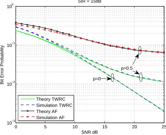
3.4.1 TWRC vs. AF:

In this section, the error rate for TWRC system and the Amplify and Forward (AF) system is measured by varying the value of SNR, while the value of SIR is kept constant.

(34)

factor β has been chosen as [43]:

β =

s

P_R

|h1|2 ·PN₁+|h2|2·PN₂+σ2 +p(1−p)

(3.19)

where σ2 and p(1−p) are AWGN and impulsive noise variance respectively. P_R,

P_N

1 and PN2are average transmission power at the relay and at the node1 and at the node2 respectively.

0 5 10 15 20 25

10−3 10−2 10−1 100

SIR = 15dB

SNR dB

Bit Error Probability

Theory TWRC Simulation TWRC Theory AF Simulation AF

p=0.5

p=0

Figure 3.4: TWRC vs. AF relay system

As expected, the TWRC system has higher performance, even when the TWRC is effected by impulsive noise with SIR=15 dB and p=0.5. This is because of network coding efficiency. The performance curve of the TWRC has more gradual slope than the AF system and less prone to the noise. It can be seen that the simulated BEP performances match the theoretical results provided by equation (3.14) very well.

(35)

words, p implies how frequently impulsive noise is added to the received signal. For example, when the value of p is equal to 1, it means that impulsive noise is consid-ered for each bit of the information stream. When pis equal to zero, it indicates that there is no impulsive noise added with the received signal.

3.4.2 BEP as function of SNR

In this section the value of SIR is changed to another value to visualize how the performance changes. For a single value of SIR, different curves are considered by changing the value of p, see Figure 3.5, Figure 3.6 and Figure 3.7.

(36)

0 5 10 15 20 25 10−3

10−2 10−1 100

SIR = 5dB

SNR dB

P=0.0 P=0.01 P=0.05 P=0.1 P=0.5 P=1

Figure 3.5: TWRC system while SIR=5 dB

0 5 10 15 20 25

10−3 10−2 10−1 100

SIR = 10dB

SNR dB

P=0.0 P=0.01 P=0.05 P=0.1 P=0.5 P=1

Figure 3.6: TWRC system while SIR=10 dB

0 5 10 15 20 25

10−3 10−2 10−1

100 SIR = 15dB

SNR dB

P=0.0 P=0.01 P=0.05 P=0.1 P=0.5 P=1

(37)

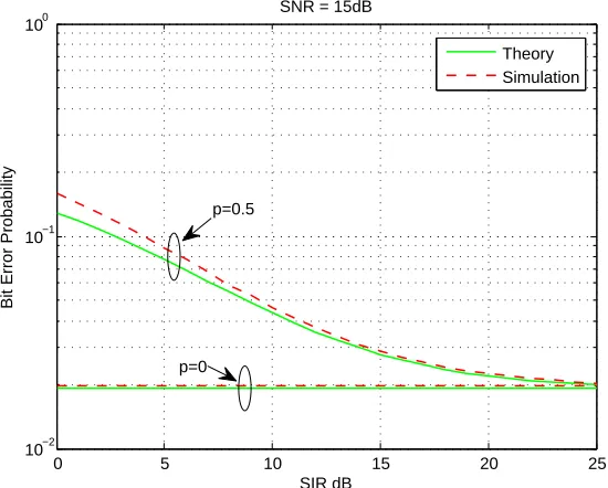
3.4.3 BEP as function of SIR

To better analyse the impact of impulsive noise on the system, performance of the TWRC system is studied in this section while varying the value of SIR and fixing the value of SNR. Figure 3.8 shows the average theoretical BEP performances and corresponding curves produced from simulations, which match the theoretical re-sults presented by equation (3.14). One interesting fact can be observed from here. Whenever the value of p is equal to zero, the performance curve is just parallel to the X-axis. When the value of pis zero, it implies that there is no impulsive noise added to the system. In such a case, there is no impact from increasing the value of SIR and the system will only experience a fixed value of AWGN which makes the curve parallel to the X-axis.

0 5 10 15 20 25

10−2 10−1 100

SNR = 15dB

SIR dB

Theory Simulation

p=0.5

p=0

Figure 3.8: TWRC system varying SIR while SNR = 15 dB

(38)

0 5 10 15 20 25 10−1

100

SNR = 5dB

SIR dB

P=0.0 P=0.01 P=0.05 P=0.1 P=0.5 P=1

Figure 3.9: TWRC system while SNR=5 dB

0 5 10 15 20 25

10−2 10−1 100

SNR = 10dB

SIR dB

P=0.0 P=0.01 P=0.05 P=0.1 P=0.5 P=1

Figure 3.10: TWRC system while SNR=10 dB

0 5 10 15 20 25

10−2 10−1 100

SNR = 15dB

SIR dB

P=0.0 P=0.01 P=0.05 P=0.1 P=0.5 P=1

(39)

figures, shows the value of pis increased, and the performance of the system be-comes worse. The saturation effect is similar to the effect described for varying SNR.

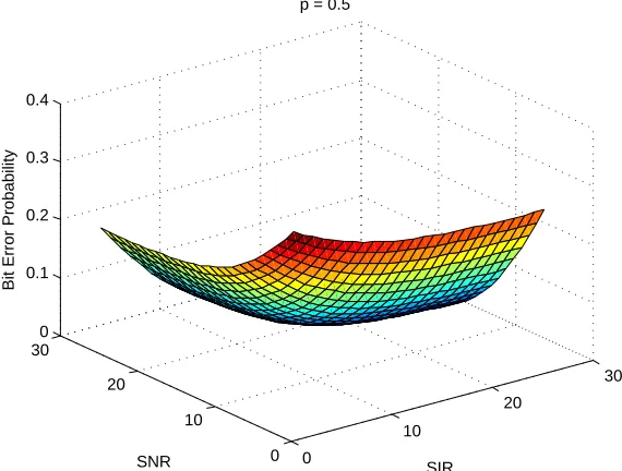
3.4.4 BEP as function of SNR and SIR

To more closely study and compare the effect of SIR and SNR, Figure 3.12 illus-trates the performance 3D graphs of the TWRC system for a fixed p = 0.5, where x, y, and z axis represent SNR, BEP, and SIR respectively. It can be observed that SIR has more deteriorative effect on the system performance than SNR.

0

10

20

30

0 10

20 30

0 0.1 0.2 0.3 0.4

SIR p = 0.5

SNR

Figure 3.12: TWRC system varying SIR and SNR while p= 0.5

(40)

3.4.5 Viterbi decoding algorithm

In this section the error rate is measured by implementing a hard decision decoding Viterbi algorithm6 [44] at the relay. I choose the rate for a convolutional encoder 1/2 with a typical generator polynomial g1(D) = 1 +D+D2 at nodes.

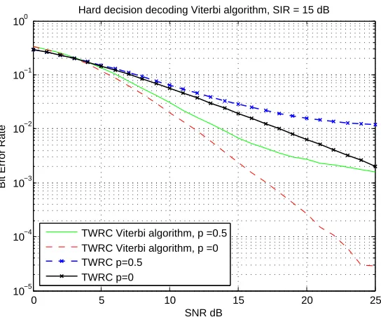
Figure 3.13 represents the performance graphs of the TWRC system with and with-out the Viterbi decoding algorithm at the relay. The simulation is done for p=0 and p=0.5. As expected, the system performance increases when I used Viterbi decoding on the relay. Note that the relay performance with Viterbi decoding for p=0.5 is even better compared to the relay without Viterbi decoding for p=0, par-ticularly for low SNR.

0 5 10 15 20 25

10−5 10−4 10−3 10−2 10−1 100

SNR dB

Bit Error Rate

Hard decision decoding Viterbi algorithm, SIR = 15 dB

TWRC Viterbi algorithm, p =0.5 TWRC Viterbi algorithm, p =0 TWRC p=0.5

TWRC p=0

Figure 3.13: TWRC system with the Viterbi decoding

(41)

3.4.6 Adaptive Coding and Modulation

For transmission of high priority data, it is more important to have a reliable link than a higher throughput link. Furthermore sometimes it is advantageous to have a higher throughput link when the channel condition is good and priority is not important. The ACM7 can get the information about data priority via coded data in the received signal, and the information about channel condition via Channel State Information (CSI) by using a pilot or embedded pilot symbol in the received signal.

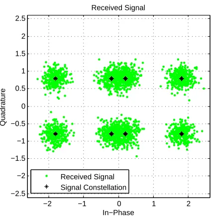
Therefore in this part Asymmetric Modulation (AM) is applied in the TWRC sys-tem and performance of the scheme is investigated. I choose a typical case, where one source node uses antipodal BPSK modulation, while the other one uses or-thogonal QPSK modulation scheme [45], Figure 3.14. The MAC transmission is the same as the symmetric scenario, but broadcast transmission will be accomplish by two sequenced BPSK transmissions to transfer a QPSK signal from 2 to node-1. Of course in this phase node-2 will get same signal twice. The relay’s

constella-N

1

R

N

2

h1 h2

g1 g1

MAC phase BC phase

BPSK QPSK

Figure 3.14: An asymmetric TWRC system

tion regions are obtained by calculation of channel gain h1 and h2, which means de-noising maping will evaluate according to the channel gain. The received signal has 8 ideal normalized constellation points, Figure 3.15.

(42)

−2 −1 0 1 2 −2.5

−2 −1.5 −1 −0.5 0 0.5 1 1.5 2 2.5

Quadrature

In−Phase Received Signal

Received Signal Signal Constellation

Figure 3.15: Constatation at relay for asymmetric TWRC BPSK and QPSK modulation

In this part, I decided that in all the following steps the relay will amplifiy the re-ceived signal by a factor of β before broadcasting, see equation (3.19). For BPSK modulation at N₁, symbols is the same as Chapter 3.3.1, but for QAM modulation atN₂, the symbols will then be (2b_k−1) +j(2b_l −1) where b_k, b_l ∈ {0,1} denotes binary information, and S_i ∈ {±1±j} for i= [1,2,3,4] denotes its symbol informa-tion. I assume both channels are affected by Rayleigh fading with AWGN with no impulsive noise environment and with |h2|>|h1|.

Figure 3.16 represents the performance graphs of the asymmetric modulation of a TWRC system for the relay and both nodes, as well as performance of the symmet-ric BPSK TWRC system.

(43)

0 5 10 15 20 25 10−3

10−2 10−1 100

SNR dB

SEP

Relay Node 1 Node 2

Symmetric BPSK TWRC, Relay

Figure 3.16: Asymmetric modulation of TWRC

For accurate comparison between two nodes, I assumed |h1|=|h2|, see Figure 3.17.

(44)

0 5 10 15 20 25 10−3

10−2 10−1 100

SNR dB

SEP

Relay Node 1 Node 2

Figure 3.17: Asymmetric modulation of TWRC when |h1|=|h2|

3.4.6.1 Optimal decision decoding algorithm (ODDA) for asymmetric

TWRC

In this section, I will propose an algorithm based on soft decision method for im-provement of received signal at one node in a asymmetric TWRC. I name the algo-rithm Optimal Decision Decoding Algoalgo-rithm (ODDA).

To present the proposed method, I have used same system as in the previous sec-tion, a QPSK and BPSK asymmetric TWRC system. The symbols for BPSK and QPSK modulations are typically given by S_{iBP SK} ={±1} and S_{iQP SK} ={±1±j}

respectively.

(45)

In conventional TWRC system, received signals at relay after decision and de-noise will be modulated and broadcasted. But in my proposal after decision and de-noise, one of the signals will be formed by XOR-ing of decoded bits of the complex re-ceived signal and the other one will be formed the same as the conventional TWRC model. In node-1 after decision, QPSK bits from node-2 will be recovered by XOR-ing. But in node-2, in the first step uses hard decision method to measures Eu-clidean distance of two sequenced received signals. In the next step decision rules apply to the signal which have least Euclidean distance. This results in decision with the highest probability for received signal, see algorithm 1.

Algorithm 1 Optimal Decision Decoding Algorithm (ODDA) for an asymmetric TWRC

M AC

N₁ : S_bpsk =±b_i N2 : Sqpsk =±bk±jbl Air

sum=S_bpsk+S_qpsk BC

T1 : real(sum)⊕imag(sum)

T₂ : real(sum)

N2

if distanceT1> distanceT2 then decision=T1>0

ˆ_b

i=decision⊕bk⊕bl else

decision=T2>0 ˆ_b

i=decision⊕bk end if

This method allows the node-2 to detect a limited number of errors that occur any-where in the signal and correct these errors without retransmission or cost.

(46)

0 2 4 6 8 10 12 14 16 18 20 10−3

10−2 10−1 100

SNR dB

BEP

BER perfomances using optimal decision algorithm

Node 2 by conventional decision Node 1 by conventional decision Node 2 by optimal decision algorithm Node 1 by optimal decision algorithm

Figure 3.18: Optimal decision decoding algorithm (ODDA) for an asymmetric TWRC

simply apply to higher order modulations in an asymmetric TWRC system.

3.4.6.2 Comparative study of BPSK and QPSK for various signal

con-stellations in a asymmetric TWRC

Finally in this section relays error probabilities studied for various signal constel-lation types depend on moduconstel-lation for each node. Simuconstel-lation have been done for antipodal and orthogonal BPSK and orthogonal and biorthogonal QPSK modula-tions. I have used the same system as in the previous section.

(47)

Case Node 2 Node 1 1 Orthogonal QP SK Antipodal BP SK

2 Orthogonal QP SK Orthogonal BP SK

3 Biorthogonal QP SK Antipodal BP SK

4 Biorthogonal QP SK Orthogonal BP SK

Table 3.1: Case study of constellations types

0 5 10 15 20 25

10−3 10−2 10−1 100

SNR, dB

SEP

case 1 case 2 case 3 case 4

Figure 3.19: Case study of constellation types for an asymmetric TWRC

3.5 Conclusions

(48)

(49)

Chapter 4 Multi antennas in a wireless TWRC

system

4.1 Introduction

In wireless communication, the effect of fading, co-channel interference and error bursts can be combatted using diversity technique via multiple antennas either at the transmitter or receiver. In this section the aim is to analyze the performance of a TWRC system in the impulsive noise environment, that uses multiple antennas at source nodes and the relay.

4.2 System model of Multiple-Input and

Single-Output TWRC

The system model of a Multiple-Input and Single-Output (MISO)1 wireless Two Way Relay Channel (TWRC) 2X1X2 is shown in Figure 4.1. To achieve transmis-sion diversity, Alamouti’s space time code [46] is used at the source nodes.

(50)

h 1,1 _h 2,1

h 2,2

h 1,2

g 1,1 g 2,1

g 1,2 g 2,2

MAC phase BC phase

R

_N

₂

N

1

Figure 4.1: A MISO TWRC system

Modulation for the system is BPSK. It is assumed that it is slow fading so that the channel gain h_k,j does not change during two consecutive time slots in each phase for all links. Let k, i, andj denote the indices of source nodes, antennas, and time slots, respectively.

MAC phase

During MAC phase, X and Y sent by N1 and N2 are as follows:

X=



 

x₁ −x∗₂ x2 x∗₁





 and Y =



 

y₁ −y₂∗ y2 y₁∗



 

respectively. The signal received by relay is:

rT =

r E1

2 h

T

1X+

r E2

2 h

T

2Y +wT +iT (4.1)

where h_k =

h_k,₁ h_k,₂ T

(51)

w = [w1, w2] is the AWGN vector at relay node with w v CN(0, σ_R2I2), where I is

an identity matrix with proper size, and at lasti = [i₁, i₂] is impulsive noise vector with i_vBern(pI₂). Assume a slow block fading and perfect channel information at the receiver.

The above transceiver signals can be rearranged as:

r=

r E₁

2 h1X+

r E₂

2 h2Y +w+i (4.2)

where: r =



 

r₁ r∗₂



 ,X =

   x₁ x₂   , Y =

   y₁ y₂   ,w =



 

w₁ w∗₂



 ,i =



 

i₁ i∗₂



 ,

h_k =



 

h_k,₁ h_k,₂

−h∗_k,₁ h∗_k,₂ 



,k= 1,2.

Indeed transmitted symbols are recovered by means of simple threshold decoders such as ML or ZF2 decoder. In this thesis I have used a ML decoder.

Lets_i denote the symbol vector constructed by the relay by XOR-ing the decoded and demapped superimposed information symbol vectors (x_i, y_i) from the source pair, i.e.,

s_i =f(x_i, y_i) = `−1((`(x_i) +`(y_i)) (modM) (4.3)

where `(z) ∈ 0,1, ..., M −1 is the label index of z in M, whereM is constella-tion size. The relay has got the CSI of the two channels, which means it knows the modulation used at each user. The maximum likelihood (ML) detection will be em-ployed at the relay according to the received signals from the MAC phase, therefore

(52)

ˆ

si can be detected as:

ˆ

s_i =arg max

s∈M

X

(X,Y):f(x_i,y_i)=s=1

exp(−D(X, Y)) (4.4) where D is the squared Euclidean distance

D(X, Y) =krT −(

r E1

2 ·h

T

1 ·X+

r E2

2 ·h

T

2.Y)k2 (4.5)

and E₁ and E₂ are transmission energy at the nodes N₁ and N₂ to R respectively. Or it can be rewritten as

D(X, Y) =k r

T

σ_R −( r

ˆ

γ

2 ·h

T

1 ·X+

r

ˆ

γ

2 ·h

T

2 ·Y)k2 (4.6)

where ˆγ =E_k/σ2 is SNR.

Now the network coding will be used to encode the estimated received signals to produce a XOR-ed signal. The XOR-ed signal will be modulate and broadcasted in the next time slot.

BC phase

During the BC phase, the modulated signal is broadcasted to both nodes. The re-ceived signal at N_k is:

(53)

The node N_k detects ˆsj as

ˆ

s_k,j =arg min

s∈M kyk,j −

p

E_k₊₂ ·g_k·sk2 (4.8) where E_k₊₂ is transmission energy at the nodesk. Each node detects the symbols sent by the other node by taking the XOR of the detected signal and its own signal:

ˆ

x_i =`−1((`(ˆs₁, j)−`(y_i)) (modM) and (4.9) ˆ

y_i =`−1((`(ˆs₂, j)−`(x_i)) (modM) (4.10) where i=j ∈1,2

4.2.1 Error probability analysis

In the system model,g_k could be modeled to be identical to or independent of h_k. Basically it depends upon the channels between N_k and R. Let us consider a sim-ple case study that can be quite easily analyzed. I assumed the channel vector g_k

is identical to h_k for k = 1,2. In addition, for analysis, I assume that h_k,i, where

k, i ∈ {1,2}and k =6 i are independent andh_k,i _v CN(0,1), i.e. Rayleigh fading channels. Let Pm denote the Symbol Error Probability or SEP in the MAC phase

for given h₁ and h₂ [47]:

Pmac , 1

(54)

In the BC phase P_bc,k denotes outage probability at S_k for given h_k:

P_bc,k _, 1

2

2 X

j=1

Pr{sˆk,j 6= ˆsj|ˆsj,hk}. (4.12)

At the relay, in a one-way transmission, if there is only one error in one of two phases, the relay is not able to detect error. But if both the phases have errors, the probability of correct detection is only _M1₋₁, where M = 2m and m = number of bits. The end-to-end SEP, is given by:

P_EtoE =Pmac+

1 2

2 X

k=1

P_bc,k − M

M −1Pmac

2 X

k=1

P_bc,k (4.13)

And the average end-to-end SEP is then ¯P_EtoE = _E[P_EtoE], with respect to the distribution of (h₁, h₂). For my simulation I have BPSK M = −1,1 andf(x, y) =

xy.

During the BC phase, the upper and lower limits for BPSK, P_bc,k is given by

P_bc,k = 1 2erfc(

q

¯

γ_k₊₂||h_k||2₎ _(4.14)

During MAC phase, the Alamouti codewords are X = [X₁,X₂,X₃,X₄] and Y =

[Y₁,Y₂,Y₃,Y₄], where X₁ =Y₁=



 

1 −1 1 1





, X2=Y2= 

 

1 1

−1 1





, X3 =Y3 = 

 

−1 1

−1 −1



 ,

X₄ =Y₄ =



 

−1 −1 1 −1



 

(55)

assumption that the exponential term with maximum argument in the sum of ex-ponentials will dominate the summation. By avoiding the sum of exex-ponentials only the exponential term remains. The approximation is widely accepted because of its relatively small performance loss.

ˆ

si =arg min

s∈{−1,1} (X,Ymin):x_iy_i=s T(X,Y). (4.15)

By considering these two mentioned issues, the following calculations derive upper and lower limits for Pmac.

4.2.1.1 Upper and lower limits of Pmac calculations

To calculate Pmac for upper-bound, assume X1 and Y1 is sent, then the

XOR-ed-like symbols is s₁ =s₂ = 1. Let

T1 = min

(X,Y):x₁y₁=1

(X,Y)6=(X₁,Y₁)

T(X, Y);

T2 = min

(56)

The derivation of error probability for s1 is:

Pr{sˆ1 =−1|(X1, Y1), h1, h2}

=Pr{min(T(X1, Y1), T1)> T2|(X1, Y1)}

=Pr{(T1 ≥T(X1, Y1))&(T(X1, Y1)> T2)|(X1, Y1)}

+Pr{(T(X1, Y1)> T1)&(T1 > T2)|(X1, Y1)}

≤Pr{T(X1, Y1)> T2|(X1, Y1)}

+Pr{T(X1, Y1)> T1|(X1, Y1)}

≤ X

(m,n)6=(1,1)

Pr{T(X1, Y1)> T(Xm, Ym)|(X1, Y1)}

= X

(m,n)6=(1,1)

P_{P EP,m,n}.

By doing the same derivation of error probability for s₂, and combining these equa-tions, the error probability for the upper bound will be determined as:

P_macU _, X

(m,n)6=(1,1)

P_{P EP,m,n} (4.16)

P_{P EP,m,n} _,Q₍_q_m_,n₎

q₍_m,n₎_,k

r

¯

γ₂

4 h

T

2(X1−X2)k, 1≤m, n≤4 (4.17)

Note thatm and n are the indices for codewords.

To calculate Pmac for lower-bound, assume that the relay is able to detect X if

¯

γ₁kh₁k2 ≥ γ¯₂kh₂k2, or Y otherwise. And if X and Y are known then: Pmac ≥ Q√γ¯₂kh₂k2 and Pmac ≥ Q

√

¯

γ₁kh₁k2 respectively, which the lower bounds of

Pmac resulting as:

P_macL _,Qqmin γ¯₁kh₁k2_,_γ_¯

2kh2k2

(57)

4.2.1.2 Upper and lower limits of end to end error probability

calcula-tions

To calculate upper and lower limits for End-to-End error probability, equation (4.13) can be defined as:

Lower bound≤P¯_EtoE ≤U pper bound max_E[P_macL ],1

2

2 X

k=1

E[Pbc,k]

≤P¯_EtoE

≤_E[P_macU ] +1 2

2 X

k=1

E[Pbc,k] (4.19)

For that we need to find _E[P_macL ], _E[P_macU ] and _E[P_bc,k].

Because khk2 is chi-square distributed with 4 degrees of freedom, hence _E[P_bc,k] =

φ(2,γ¯_k₊₂) where from [42], equation (14-4-15):

φ(L, ρ)_,

h1−µ(ρ)

2

iLLX−1

l=0

h1−µ(ρ)

2

il

µ(ρ)_,

r _ρ

1 +ρ (4.20)

Because (X₁−Xm) and (Y1−Ym) are both orthogonal matrices, we have:

qm,n =pα¯m,n ηm,nT (4.21)

where ηm,n = [ηm,n,1, ηm,n,2]T vCN(0,I2).

The ¯αm,n can be found from table 4.1. The value of ¯αm,n has been calculated for

(58)

mn 1 2 3 4 1 − γ¯₂ 2 ¯γ₂ γ¯₂ 2 γ¯1 γ¯1+ ¯γ2 γ¯1+ 2 ¯γ2 γ¯1+ ¯γ2

3 2 ¯γ₁ 2 ¯γ₁+ ¯γ₂ 2 ¯γ₁+ 2 ¯γ₂ 2 ¯γ₁+ ¯γ₂

4 γ¯₁ γ¯₁+ ¯γ₂ γ¯₁+ 2 ¯γ₂ γ¯₁+ ¯γ₂

Table 4.1: Values of ¯αm,n P_EtoE.

The average PEP is given by _E[P_EEP,m,n] = φ(2,₂1.α¯m,n), where thePmacU from

equation (4.16) is given by P_macU _, P

(m,n)6=(1,1)φ(2,

1

2.α¯m,n), where 1

2 is from

equation (4.17). Now the upper bound of ¯P_EtoE can found as:

¯

P_EtoEU _,_E[P_macU ] +1 2

2 X

k=1

E[Pbc,k] =

X

(m,n)6=(1,1)

1≤m,n≤4

φ(2,1

2 ·α¯m,n) + 1 2

2 X

k=1

φ(2,γ¯_k₊₂)

(4.22) Now if taken into account impulsive noise (equation (2.10)) will give:

¯

P_EtoEU _,p X

(m,n)6=(1,1)

1≤m,n≤4

φ(2,1

2·α¯m,n) + 1 2

2 X

k=1

φ(2,¯γ_k₊₂)+

(1−p)

_X

(m,n)6=(1,1)

1≤m,n≤4

φ(2,1

2·α¨¯m,n) + 1 2

2 X

k=1

φ(2,γ¨¯_k₊₂)

(4.23)

where ¨α¯m,n and ¨γ¯k+2 are calculated on account of the sum of impulsive and

addi-tive white Gaussian noise.

For the lower bound of ¯P_EtoE, we need to find _E[P_macL ]. I assume:

γ_k = ¯γ_kkh_kk2, k= 1,2

(59)

The CDF3 of γ_k isF_γk(ξ) = 1−e−

ξ

¯

γk ₋ ξ

¯ γ_ke

−_¯ξ

γk_{, which yields to the PDF of}_β _as

f_β(ξ) =c₁ξe−

ξ

¯

γk + c2

2¯γξ2e

−_¯ξ

γk. Hence we will have

E[PmacL ] =c1¯γ2φ(2,

¯

γ

2) +c2¯γ

2

φ(3,¯γ

2) (4.24)

where c1 ,

1 ¯

γ₁2 +

1 ¯

γ₂2, c2 ,

2 ¯

γ₁γ¯₁, γ¯, ¯

γ1γ¯2

¯

γ₁+ ¯γ₂

Now we can find lower bound on ¯P_EtoE by substituting in equation (4.19) as

¯

P_EtoEL _,max_E[P_macL ], 1

2

2 X

k=1

E[Pbc,k]

=maxc₁γ¯2φ(2,γ¯

2) +c2γ¯

2_φ₍₃_,γ¯

2), 1

2φ(2,¯γ3) +φ(2,γ¯4)

(4.25)

Now if taken into account impulsive noise (equation (2.10)) will give:

¯

P_EtoEL _,p

max

c1¯γ2φ(2,

¯

γ

2) +c2¯γ

2

φ(3,¯γ

2), 1

2φ(2,γ¯3) +φ(2,γ¯4)

+

(1−p)maxc₁γ¨¯2φ(2,¨¯γ

2) +c2¨¯γ

2_φ₍₃_,¨¯γ

2), 1

2φ(2,γ¨¯3) +φ(2,γ¨¯4)

(4.26)

where ¨¯γ, ¨¯γ3 and ¨γ¯4 are calculated on account of the sum of impulsive and additive

white Gaussian noise.

Finally by driving the upper and lower limits for error probability we can prove the simulation of the Alamouti wireless Two Way Relay Channel system.

(60)

0 2 4 6 8 10 12 14 16 18 10−4

10−3 10−2 10−1 100

SNR, dB

SEP

Upper bound of Error Probability for p=0 Lower bound of Error Probability for p=0 Simulation of Error Probability for p=0

Figure 4.2: Upper and lower bounds when p = 0 and SIR = 10 dB

0 2 4 6 8 10 12 14 16 18

10−4 10−3 10−2 10−1 100

SNR, dB

SEP

Figure 4.3: Upper and lower bounds when p = 1 and SIR = 10 dB

4.2.2 Simulations and results

4.2.2.1 SEP as function of SNR

Figures 4.2 and 4.3 show the simulation of SEP while the value of the SIR is kept constant 10 dB for the casesp = 0 and p = 1. Obviously we see when p = 1, the performance of the system deteriorates. The figures also show the upper and lower bounds according to the equations (4.23) and (4.26) respectively. The agree-ment between the analytical bounds and simulated SEPs for the system shows that derived bounds can predict the performance well. The figure shows that the simu-lation curve is closer to the lower bound than the upper bounds. The reason is that the approximation in theoretical calculation for the upper-bound result to less accu-racy compare to the lower-bound.

4.2.2.2 SEP as function of SIR

(61)

0 2 4 6 8 10 12 14 16 18 10−2

10−1 100

SNR, dB

SEP

Figure 4.4: Upper and lower bounds when p = 0 and SNR = 5 dB

0 2 4 6 8 10 12 14 16 18

10−2 10−1 100 101

SNR, dB

SEP

Figure 4.5: Upper and lower bounds when p = 1 and SNR = 5 dB

p = 0 and p = 1. Obviously when p = 0, the performance curve is parallel to the X-axis and depends only on the value of SNR, which is fixed. Whenp = 1 the performance of the system becomes worse.

4.2.2.3 Comparison

(62)

is a double4 of that between a source node and the relay in system-2.

Figure 4.6 shows obviously that system-3 performance is better than system-1 be-cause of higher diversity gain at system-3. In addition the Alamouti schemas out-performs single antenna relay as well when the impulsive noise is high. As the

Fig-0 2 4 6 8 10 12 14 16 18

10−4 10−3 10−2 10−1 100

SNR, dB

SER

Relay Alamouti 2x1, p=0

Lower bound relay Alamouti of PEtoE, p=0 Relay Alamouti 2x1, p=0.5

Upper bound relay Alamouti of PEtoE, p=0.5 MIMO 2x1, P=0

MIMO 2x1, P=0.5 Single antenna relay, p=0 Single antenna relay, p=0.5

Figure 4.6: Performance comparison of different systems, SIR = 10 dB

ure shows system-3 performs better than system-2 since in system-3 the relay de-noise and forward signals, while in system-2 the relay just transfers signals directly. It is interesting to note that the system-2 performance is better than the system-1 performance.

4. Let the transmitted signal power beP t, and the received power be P r. Let the fre-quency denoted byf, and cbe the speed of light. The distance between the transmitter and receiver isD. Let Gt and Gr represent the transmitter and receiver antenna gains re-spectively. The upper limit of the power received, when power P tis transmitted is given by the Friis formula, which accounts for the free space path loss Pr = PtGtGr

c

4πDf

2

.

(63)

4.3 System model of Multiple-Input and

Multiple-Output TWRC

The system model of a Multiple-Input and Multiple-Output (MIMO) wireless Two Way Relay Channel (TWRC) 2X2 is shown in Figure 4.7 [48]. In this system the

MAC phase BC phase

R

_N

₂

N

1

h i,j,k h i,j,k

g i,j,k g i,j,k

Figure 4.7: A MIMO TWRC system

nodes and the relay are each equipped with two antennas to improve the trans-mission quality. Letx_i,j, i, j = {1,2} denote the symbol transmitted by the jth antenna of node N_i, i = {1,2}, which is represented by matrix X_i. The received symbol matrix Yr at the relay can be written as

Yr= s

E₁

A_N₁H1 Xi+ s

E₂

A_N₂H2 Xi+Wi+Ii (4.27)

where H_i is the fading channel coefficient matrix with elements h_i,j,k, from node

Ni’s jth antenna to the relay’s kth antenna, and Wi and Ii are the AWGN and

im-pulsive noise matrix respectively at the relay’s jth antenna. A_N_i is the number of antennas at node N_i, which in our case is 2, and E_i is transmitting energy at node

(64)

The relay decodes the received symbol using ML decision to obtain ˆxi,j. After

net-work coding we get ˆxˆ_i,j, which the relay after modulation broadcasts to both nodes. Thus at the broadcast phase, nodeN_i receives

Y_i =

s Er A_RGi

ˆ ˆ

X_i+W_i+I_i (4.28)

where Y_i receives the signal matrix at nodeN_i, and G_i is the fading channel coeffi-cient matrix with elements g_i,j,k, from the relay’s kth antenna to the node N_i’sjth antenna. A_R is the number of antennas at the relay, which in our case is 2, and Er

is transmitting energy at the relay.

Finally the nodes N_i perform ML decoding and extracts transmitted symbols from the other terminal with its own symbols.

4.3.1 Simulations and results

(65)

0 2 4 6 8 10 12 14 16 18 10−4

10−3 10−2 10−1 100

SNR,dB

End−to−end bit error probability

2X1 TWRC, p=0 2X1 TWRC, p=0.5 2X2 TWRC, p=0 2X2 TWRC, p=0.5

Figure 4.8: MIMO TWRC system vs. MISO TWRC system

4.4 Conclusions

(66)

Part II

(67)

Chapter 5 Polarized antennas in a wireless TWRC

system

5.1 Introduction

The next generation wireless TWRC system will demand high data rate services to meet requirements from various applications [49]. In this chapter, I propose a new TWRC scheme based on polarization, which is able to transmit and receive data between nodes simultaneously, in other words full duplex system, by using the same carrier frequency.

5.2 Polarized Antenna Network Coding (PANC)

and full duplex PANC

Until now the half duplex wireless TWRC system has been analyzed, which suffers from time delay, since relay nodes have to wait until adjacent nodes complete their transmission, because in the time domain there is only one channel for transmis-sion. This also affects the spectral efficiency, because in the time domain, half of data transmission capacity is available in both directions.

(68)

the number of channel resources get doubled, since the available spectrum is scarce and expensive. It is not a good approach. The other disadvantage to having two carrier frequencies is related to the synchronization issue that exists between the relay and the nodes, which increase complexity of the system synchronization. However here I propose a new scheme to achieve a full duplex transmission system and decrease transmission delay, while using the same carrier frequency, which I call Full duplex Polarized Antenna Network Coding (PANC), Figure 5.1.

Network Coding (NC)

Analogue Network Coding

(ANC)

Digital Network Coding

(DNC) Spatial

Multiplexing Network Coding

(SMNC)

Polarized Antenna Network

Coding (PANC) Spatial Antenna

Network Coding (SANC)

Diversity Multiplexing Full duplex PANC

Figure 5.1: Network coding

Horizontal, vertical, left- and right-hand circular polarized transmissions will not interfere with each other, because they are differently polarized. This means sig-nals via same carrier frequency can be transmitted and received simultaneously by different polarizations via a transceiver.