Removing Striping Noise from Cloudy Level 2 Sea
Surface Temperature and Ocean Color Datasets
Boussidi Brahim1,∗, Fablet Ronan1and Chapron Bertrand2
1 Institut Mines Télécom - Télécom Bretagne
UMR 6285 LabSTICC CS 83818 - 29238 Brest Cedex 3 - France
2 Laboratoire d’Océanographie Physique et Spatial (LOPS), IFREMER
Centre Bretagne - ZI de la Pointe du Diable - CS 10070 - 29280 Plouzané
* Correspondence: [email protected]
Abstract: This paper introduces a new destriping algorithm for remote sensing data. The method is based on combined Haar Stationary Wavelet transform and Fourier filtering. State-of-the-Art methods based on the discrete wavelet transform (DWT) may not always be effective and may cause different artifacts. Our contribution is three-fold: i) we propose to use the Undecimated Wavelet transform (UWT) to avoid as much as possible shortcomings of the classical DWT; ii) we combine a spectral filtering and UWT using the simplest possible wavelet, the Haar basis, for a computational efficiency; iii) we handle 2D fields with missing data, as commonly observed in ocean remote sensing data due to atmospheric conditions (e.g., cloud contamination). The performances of the proposed filter are tested and validated on the suppression of horizontal strip artifacts in cloudy L2 Sea Surface Temperature (SST) and ocean color snapshots.
Keywords:Destriping; Undecimated wavelet transform; Fourier filtering; Sea Surface Temperature; Ocean color
1. Introduction
Passive sensors on board remote sensing platforms use several scanning methods to generate land and sea surface imagery. Images provided by the Sun-synchronous Earth orbit satellites are achieved by a combination of progressive scanning lines in the cross-track direction while the sensor platform motion is along the in-track direction. The resulting images are often contaminated by several types of noise. These undesired artifacts have a direct impact on the visual quality of the provided images. If not corrected, these noises will then further cause processing errors. In this paper, we will deal with striping noise patterns. This type of noise are often present in sea surface temperature and ocean color images provided by infrared and optical imaging spectrometers (e.g. MODIS, VIIRS...). It consists in sharp repetitive patterns which take the form of stripes over the entire
image [1] (See Fig.1).
The reduction of these stripe artifacts is an important research topic. A large number of
destriping algorithms have been recently suggested. All the scene-based methods of the destriping
literature exploits geometrical priors about the noise. These priors are related to the regular
periodicity of the noise. One may cite a variety of approaches based on low-pass filtering
implemented in the spatial or frequency domain [2–6]. A common feature shared by these methods
is that they give rise to blur artifacts. More sophisticated filtering approaches have been proposed.
Multiresolution analyses using wavelet decompositions were investigated in [7,8]. More recently,
variational methods were introduced and explored in [9,10]. These methods may however be
prohibitively expensive for large datasets.
Reducing striping artifacts in an effective manner without blurring the images still remains challenging. Moreover, the considered case-study applications, infrared sea surface temperature
and ocean color observations [11], do not involve cloud-penetrating sensors, What may result in a
address the removal of striping noise in ocean remote sensing images, possibly involving missing
data as illustrated in Fig.1. We develop a destriping algorithm based on a combined wavelet-Fourier
filtering. Our algorithm can be regarded as an extension of [7]. We evaluate our contribution for real
ocean satellite-derived images with a focus on both SST and ocean color imagery.
This paper is organized as follows. In section2, we provide a short review of the assumptions
required by the wavelet decomposition and Fourier transform. In section 3, a detailed technical
description of the proposed destriping algorithm is given. We report numerical experiments with
real ocean remote sensing data, including a comparison to state-of-the-art approaches in Section4.
Section5concludes this paper.
−0.25 −0.2 −0.15 −0.1 −0.05 0 0.05 0.1 0.15 0.2 0.25
13.2 13.4 13.6 13.8 14 14.2
(a) (b)
(d) (e) (f)
(c)
Figure 1. Destriping of an ocean brightness temperature snapshot obtained by TIRS Lanndsat 8 on September 11, 2014. The original data are shown in panel (b) while the destriped data are shown in
panels (b), (d), (e) and (f) using respectively our method, [7] with Haar wavelet, [7] with Daubechies-4
and using a variationnal approach proposed by [10].
2. Problem statement
Let us consider an observed imageusn(i)defined in a rectangular domaini∈ Ω, affected by an
additive stripe-type noise. The image degradation model can be expressed by the following equation
usn(i) =u(i) +sn(i) (1)
whereu(i)would be the true value at pixeliandsn(i)is the striping noise perturbation. The analysis
of satellite images shows that the striping noise can be considered as a structured noise in which the
large variability is along theyaxis of the image, as illustrated in Fig.1.
By exploiting this prior on the spatial structure of the undesired noise, the filtering problem consists in removing the striping noise of the images without introducing any blurring effects.
Following [7], the proposed approach relies on an appropriate decomposition of the image usn(i)
so that the striping noise effect can be isolated from the original hidden image. Notice that we will not deal with other stationary noise, which may be present in the images and removed using appropriate methods. Several filtering approaches have been developed for the removal of striping noise in satellite images. Following the idea that striping noise is a superposition of quasi-perfect periodic signals and can be easily identified in the 2D Fourier spectrum, one can construct a filter
the fact that this filter does not only remove part of the spatial frequency component related to the undesired stripe noise, but also eliminates and reduces the part of the same component present in the
real (physical) signal. In order to avoid this over-denoising effect, [7] proposes to perform this spectral
filtering method after a first finite-level discrete dyadic wavelet transform. In this algorithm only the wavelet coefficients (details) are assumed to contain the undesired striping noise and are filtered in the Fourier domain. All the approximation coefficients are kept and the resulting image is obtained by the inverse wavelet transform using the denoised coefficients. The decimated Wavelet analysis (DWT) takes advantage of scaling and directional properties to detect and remove striping patterns in the
wavelet domain. The DWT is a non-redundant decomposition [12]. This is particularly interesting for
storage and computational efficiency purposes. Nevertheless, for reconstruction-related applications, which is our use case here, the DWT does not fulfill the translation-invariance property, what may lead to a large number of artifacts when modifying its wavelet coefficients.
3. Proposed destriping approach: THE UWT-Fourier based destriping scheme
Following [7], we propose to tackle the problem of removing striping noise through a combined
wavelet-Fourier approach. As previously mentioned, destriping with the traditional (orthogonal) discrete wavelet transform sometimes exhibits visual artifacts. These artifacts are caused by the
sensibility of these algorithms to translation. The Undecimated wavelet transform (also called
stationary wavelet transform) was designed to overcome the lack of translation-invariance of the
DWT [12]. This property is achieved by removing the decimation step in the orthogonal wavelet
transform.
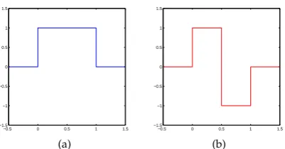
Haar-based UWT decomposition: In the proposed Desptriping scheme, the 2D Haar wavelet transform is the proposed analysis technique. The Haar basis function is well known as the first and the simplest wavelet analysis. The associated scaling and wavelet functions (denoted respectively by
φ(x)andρ(x)) are illustrated in Fig.2.
The major advantages with the use of the Haar analysis are the following:
1. Interpretability: the form of Haar filter is simple and easy to implement;
2. Computational efficiency: unlike the continuous wavelets, fast calculations are obtained, which is important for large satellite derived data products;
3. The inverse transform is performed without any edge effect artifacts. This a key feature in our case as we deal with images involving missing data.
Notice that for applications where reconstruction is needed, the Haar transform also has limitations. Images reconstructed with the Haar filter may exhibit block-like artifacts when the decimation is involved. The considered UWT approach resolve this problem.
The original imageusn is represented in the UWT domain by a sequence of details at different
scales and orientations along with an approximation image at a predefined coarsest scale.
˜
U= (U0J,UJ−1,· · ·,U1) (2)
where U0J represents the approximation image at the lowest scale J and Uk,k = 1· · ·J −1
represent the detail images at levelk. Each of these component consists of three orientation bands
Uk=hUk v,Uhk,Udk
i
. The original image can be obtained using its coefficients by the inverse UWT.
Fourier filtering:We assume that the noise is periodic, invariant along the x-axis and distributed
over several spectral component. Given the Haar UWT decomposition of the noisy imageusn, we
−0.5 0 0.5 1 1.5 −1.5
−1 −0.5 0 0.5 1 1.5
(a)
−0.5 0 0.5 1 1.5 −1.5
−1 −0.5 0 0.5 1 1.5
(b)
Figure 2. The Haar filter. (a) Scaling Function (low-pass filter) and (b) Wavelet function (High-pass filter)
components Usni,v,d. Let us denote by gα the considered filter in the Fourier domain. The filtered
detail image for band(i,k)is given by
F−1(gα× F U
j,k
sn) (3)
whereF andF−1refer, respectively, to the Fourier and the inverse Fourier transform. The denoised
image ˜uthen resorts to
˜
u(i) =W−1(U0
sn,Usn1,h,· · ·,Usnd,h,F−1(gα× F U
j,k
sn)j=1:n) (4)
whereW−1is the inverse UWT transform,jandkare, respectively, the scale level and the orientation
of the wavelet subband.
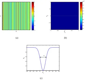
Fourier filter design: In the 2D wavenumber domain~k = (kx,ky) the ideal horizontal (resp. vertical) stripes are almost located near the high frequency part in the vertical (resp. horizontal)
direction, i.e(0,ky)[see Fig.3for an illustration]. The destriping Fourier filter is designed to remove
this wavelengths from the Fourier transform of the noisy UWT coefficients. For this purpose, we
apply a band-pass filter aroundky = 0. This can be achieved by the pointwise multiplication of the
FFT coefficients with an inverted Gaussian function
g(kx,ky) =1−exp(−kx/σ2) (5)
whereσcontrols the width of the filter in thekx-direction. Fig.3shows an example of such a function.
Since the observed striping artifacts are almost horizontal (resp. vertical), the value ofσmust be small
so that the Fourier coefficients are set to zero only atkx = 0 (resp. atky =0). Thereby, the filtering
process is expected to eliminate striping artifacts without producing blur effects.
We define the method noise ofuas the image difference
ns(i) =usn(i)−u˜(i) (6)
This method noise (or noise residue) should be as similar as possible to an image composed only of striping patterns.
X Y −3 −2 −1 0 1 2 3 (a) kx ky
−1 −0.5 0 0.5 1
−1 −0.5 0 0.5 1 0.2 0.4 0.6 0.8 1 1.2 1.4 1.6 1.8 2
x 104
(b)
−2500 −200−150−100 −50 0 50 100 150 200 250 0.2 0.4 0.6 0.8 1 gα k x α (c)
Figure 3. (a) A simulated perfect vertical Gaussian striped sheet. (b) The associated 2D power spectrum. All non-zero values are located near the high frequency part in the horizontal direction (c) The inverted Gaussian function considered as the Fourier filter in our algorithm
which will result in no noticeable discontinuities of the denoised image at the boundaries of missing
data areas. For this purpose, we consider the harmonic image inpainting as described in [13]. The
method smoothly interpolates inward from the pixel values on the outer boundary of the missing regions. In the following, we will briefly explain the method. Let us consider an image denoted by
f and defined in a rectangular domain denoted byΩ. Suppose that this image is only known at a
subsetΩk ⊂Ω. The harmonic inpainting method consists in filling in the missing region by solving
the following Dirichlet boundary value problem
∆u = 0 on Ω\Ωk
u = f on Ωk
∂nu = 0 on ∂Ωk
(7)
where∂ndenotes the derivative operator normal to the boundaries. We can also consider higher-order
differential operators as interpolant (e.g., the biharmonic operator∆2).
4. Experimental Results
Experimental setting: Several BT, SST and ocean color snapshots acquired by MODIS
Aqua/Terra [14], VIIRS NPP [15] and TIRS Landsat8 [16] were selected to illustrate and validate
the performance of the proposed algorithm. We choose scenes heavily affected with striping noise.
Examples of destriping The visual improvement of Modis-Terra ocean color snapshots is
illustrated in Fig.4and Fig.5. Smaller images (≈ 400×400 pixels) compared to the entire received
0 1 2 3 4 5 6 7 8 10 12 14 16 18 20 log(Wavelength) log(Spectrum) Original image Destriped image 0 0.1 0.2 0.3 0.4 0.5 0.6 0.7 0.8 0.9 1 0 0.1 0.2 0.3 0.4 0.5 0.6 0.7 0.8 0.9 1 −0.25 −0.2 −0.15 −0.1 −0.05 0 0.05 0.1 0.15 0.2 0.25
(a) (b) (c)
(d) (e) (f)
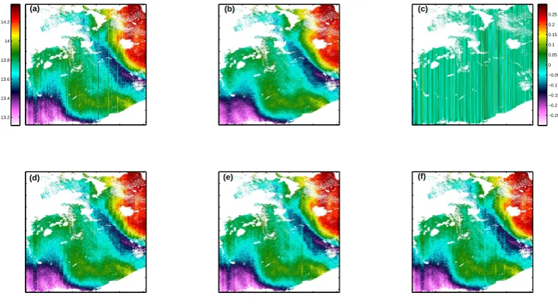
Figure 4. Illustration of the destriping of ocean color products: (a) chlorophyll-a concentration obtained by Modis Terra on December 22, 2015 around 06:20 UCT in the Arabian sea region. The destriped data are shown in panel (b). The gradient magnitude of the original image and the destriped image are shown respectively in panel (d) and (e). Comparison of the averaged Fourier power spectrum is illustrated in panel (f).
0 1 2 3 4 5 6 7 9 10 11 12 13 14 15 16 17 18 19 log(Wavelength) log(Spectrum) Original image Destriped image 0 0.1 0.2 0.3 0.4 0.5 0.6 0.7 0.8 0.9 1 −0.25 −0.2 −0.15 −0.1 −0.05 0 0.05 0.1 0.15 0.2 0.25 0 0.1 0.2 0.3 0.4 0.5 0.6 0.7 0.8 0.9 1
(a) (b) (c)
(d) (e) (f)
effect. Fronts and sharp gradients areas are degraded by stripe noise in the original images. This occurs because stripes lead to larger vertical gradients. These geometrical features are significantly
enhanced in the resulting destriped snapshots. In panels Fig.4(f) and Fig.5(f), we plotted the averaged
Fourier power spectrum. The stripes are revealed in the Fourier spectrum by several impulses (or pics) located at different wavelengths, often at Mid and High frequency components. We can observe from the analysis of the the spectral densities before and after the destriping process that striping noise components are no more observed in the spectra of the processed images.
We also applied our algorithm to SST snapshots provided by Modis sensor onboad Aqua
platform. As shown in Fig.6, we reported similar to those obtained for ocean colour snapshots.
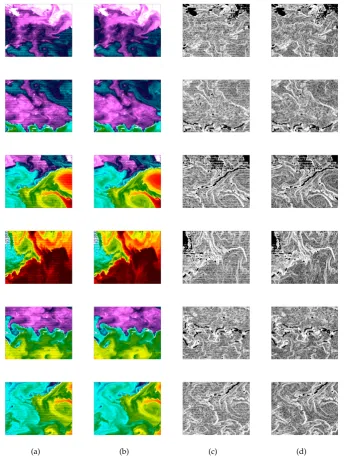
(a) (b) (c) (d)
Figure 6.Illustration of the destriped results for SST snapshots derived from Aqua Modis sensor.(a) Original images (b) Destriped images with the proposed algorithm. (c) Gradient magnitude of the original fields. (d) Gradient magnitude of the Destriped images
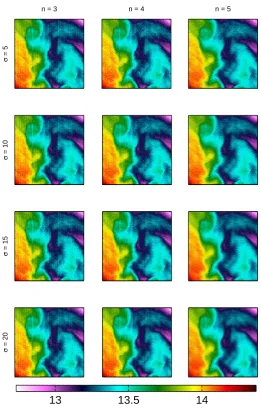
transform do have an effect on the quality of the obtained images. Fig.9 shows the joint influence of these key parameters. It suggests that the typical variance parameter must be small. Large values produce a blurring effect. In the various results illustrated in this paper, the default value
for the σ parameter is set to 5. Notice that even with smaller values the algorithm gives good
performances. Regarding the UWT, a suitable number of decomposition shall not exceed 5 levels. To deal with the missing data issue while using the Fourier filtering, our method uses a preprossing
step which consists in filling in the missing areas using the Laplacian inpainting method. Fig.8
stresses the benefit of such an interpolant comparing with the classical zero-padding method. This method has been chosen for a practical considerations, since it is parameter-free and inexpensive in computer storage space (relatively sparse matrices to invert) compared to inpainting method based on high-order differential operators (e.g., biharomic inpainting). This method is especially suitable for images involving high rate of missing data where the discretisation of the Laplcian operator gives rise to large matrices. From the reported experiment here using a bi-harmonic interpolant, we expect
other inpainting methods based in diffential operator (e.g., AMLE [13]) to lead to similar destriping
performances, at the expense of an increased computational complexity.
Comparison to state-of-the-art algorithms:
We performed a comparisons to two recent state-of-the-art algorithms, namely the
Fourier-wavelet scheme proposed by [7] and the non-local variational approach proposed by [10].
Compared to our approach, [7] uses the decimated wavelet transform (DWT) which is less
effective, especially in the heavy stripped image. In addition, the use of the Haar filter is not suitable and the number of taps (i.e., nonzero coefficients) for the chosen wavelet form must be large. This
is illustrated by the results reported in Fig.9. The quality of the image generated by our method is
superior to the images obtained using [7]. Unlike panels Fig.9(d)-(e), all the stripes was removed and
the image contains no artifacts.
Fig.9also shows the improved destriping performance of our algorithm compared to [10]. We
further compare in Fig.10 the method noise resulting from our algorithm and [10]. The visual
inspection of the associated Fourier power spectra shown in panels Fig.10(c)-(d) suggests that the
energy of our method noise is almost distributed in the narrow horizontal wavenumbers band near
ky = 0. By contrast, the energy related to the method noise of the destriped image using [10] is
distributed over a broad spectral band and does not conform to the prior assumption about the geometrical nature of the undesired noise. A direct impact of this observation can be seen in the
averaged Fourier spectrum reported in panel Fig.10(e). In fact, The signal spectral magnitude is
attenuated for frequencies located near the mid-wavenumber region.
To achieve a quantitative comparison with the considered sate-of-the-art methods for the ocean color maps we compute the mean of the cross-track profiles of each image. This quantitative metric measurement gives a good indication of the strength of the striping noise present in a given image. It consists in calculating the average value along each scan line. The presence of stripes translates to the mean cross-track profile by a strong periodicity. Using this metric, the goodness of a given destriping algorithm is described in terms of its ability to remove this periodic component and obtain
a smooth signal. We plot in Fig.11 the cross-track profiles of images displayed in Fig.4 and Fig.5.
As expected, the original destriped image exhibits a strong periodicity. The profiles of the destriped
images using our approach as well as [7] and [10] are also reported. While our approach and [7] resort
to slow-varying profiles with no periodic pattern, [10] does not sufficiently remove these periodic
components which are still visible at the end of the scan.
Impact of the destriping for the analysis of SST and Ocean Color snapshots: We illustrate the potential of the proposed destriping algorithm for an operational use of the resulting sea surface fields. The first application deals with the application of our algorithm as a preprocessing step in
the automatic detection of SST fronts [17]. For this purpose, we apply a Sobel filter to a subset of an
original Modis SST maps at full sensor resolution of≈ 1km and using a downsampled resolution
σ
= 5
n = 3 n = 4 n = 5
σ
= 10
σ
= 15
σ
= 20
13
13.5
14
Figure 7.Destriping results of the image shown in Fig.5.1(a) for different values of the variance related
13.2 13.4 13.6 13.8 14 14.2
(b) (c)
(a)
Figure 8. Destripng results of the image shown in Fig.5.1(a) using different method for filling the missing areas before destriping; (a) zero-padding; (b) harmonic inpainting (c) biharmonic inpainting.
13.2 13.4 13.6 13.8 14 14.2
−0.25 −0.2 −0.15 −0.1 −0.05 0 0.05 0.1 0.15 0.2 0.25
(a) (b) (c)
(d) (e) (f)
Figure 9.(a) Original brightness temperature image from TIRS Landsat 8. (b) Destriped image using
our method. (c) The removed residual component. (d) Destriped image with [7] using Haar function.
−0.1 −0.08 −0.06 −0.04 −0.02 0 0.02 0.04 0.06 0.08 0.1 (a) (b) ky kx
200 400 600 800 1000 100 200 300 400 500 600 700 800 900 1000 (c) kx ky
200 400 600 800 1000 100 200 300 400 500 600 700 800 900 1000 (d) 1 1.2 1.4 1.6 1.8 2 2.2 −12.5 −12 −11.5 −11 −10.5 −10 −9.5 log(Wavelength)
log(Spectrum) Original image
(b) (e) (f)
(e)
Figure 10. The method noise of the original image shown in Fig9associated to (a) Our method (b)
[10]. Panel (c) and (d) report respectively the Fourier power spectrum of (a) and (b). The averaged
Fourier power spectrum of the obtained results in Fig9are plotted in (e), the legend inside refers to
Fig.9
50 100 150 200 250 300 350 400 0.2 0.25 0.3 0.35 0.4 0.45 0.5 Line number Mean profile Original image Destriped with our method Combined DWT−Fourier (db4) Variational approach
perform the same operation using the destriped version of the considered image. Fig.12illustrates the results obtained for this experiment. As expected, in both the full and downsampled resolution of the real image, strong gradients are exhibited for real SST fronts and also caused by the vertical stripes. As such, an automatic detection algorithm would hardly be able to discriminate these two classes of gradient patterns. By contrast, the effect of the destriping is clear in the processed images. It reveals more clearly the geometry of the SST fronts, which were occluded in some cases by the striping artifacts. This example illustrates that our destriping scheme can enhance the detection of thermal fronts using simple automatic front detection algorithms.
(a) (b)
(c) (d)
Figure 12. Illustration of the impact of the striping noise in the detection of thermal fronts from SST snapshots. The magnitude gradient field of a Modis snapshot computed using the Sobel operator using (a) the full image resolution (b) downsampled version at 4km (c) destriped image at the full sensor resolution (d) the destriped image at 4km resolution.
The retrieval of Level-2 SST products from a Level-1 brightness temperature data may be
considered as a second potential use of the proposed destriping approach. The linear [18] (resp.
nonlinear [19]) SST retrieval algorithms are typically based on linear (resp. nonlinear) combination
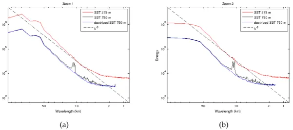
of brightness temperature extracted from several channels. Brightness temperature datasets are also involved with stripe artifacts. Thus, it is more convenient to reduce stripe noise before performing the retrieval. Here we report such an application using VIIRS data. Brightness temperatures from the 375 m resolution Imagery Bands (I-Band) are used with 750 m resolution SST fields obtained from the VIIRS Moderate Resolution Bands (M-Band) to obtain 375 m SST fields. The algorithm consists in
computing regression coefficients by a rolling-window analysis. We report two examples in Fig.13.
They illustrate the benefits of the destriping prior to the application of SST retrieval algorithm.
5. Conclusion
(a) VIIRS SST 750 m (b) Destriped SST 750 m (c) VIIRS SST 375 m
Figure 13.Illustration of the potential use of the proposed destriping algorithm. The destriped VIIRS SST data are used along with the I-Band BT at 375 m to produce SST product at 375 m.
(a) (b)
combines a UWT decomposition of the image to a Fourier filter. Contrary to most state-of-the-art techniques, this proposed scheme can very efficiently deals with missing data. On different real satellite-derived images, we demonstrated the relevance of the proposed approach compared to previous work. The use of the UWT is regarded as a key component, which brings clear benefit
compared to the DWT [7] and variational prior [10]. As illustrated, we anticipate the impact of the
proposed destriping scheme for the further analysis of satellite-derived sea surface fields, especially to analyze signatures of sub-mesoscale upper ocean dynamics.
Acknowledgments: This work was supported by ANR (Agence Nationale de la Recherche, grant ANR-13-MONU-0014), Labex Cominlabs (grant SEACS).
Author Contributions:B.B. designed and performed the experiments; R.F. and B.C. contributed to the analyses; B.B., R.F. and B.C. wrote the paper.
Abbreviations
The following abbreviations are used in this manuscript:
SST Sea Surface Temperature
BT Brightness temperature
MODIS Moderate Resolution Imaging Spectroradiometer
VIIRS Visible Infrared Imaging Radiometer Suite
NPP National Polar-orbiting Partnership
TIRS Thermal Infrared Sensor
FFT Fast Fourier Transform
DWT Discrete Wavelet Transform
UWT Undecimated Wavelet Transform
Bibliography
1. Simpson, J.J.; Yhann, S.R. Reduction of noise in AVHRR channel 3 data with minimum distortion. IEEE
Transactions on Geoscience and Remote Sensing1994,32, 315–328.
2. Srinivasan, R.; Cannon, M.; White, J. Landsat Data Destriping Using Power Spectral Filtering. Optical
Engineering1988,27, 271193–271193–.
3. Crippen, R.E. A simple spatial filtering routine for the cosmetic removal of scan-line noise from Landsat
TM P-tape imagery. Photogramm. Eng. Reote Sens1989,55, 327–331.
4. PAN, J.J.; CHANG, C.I. Destriping of Landsat MSS images by filtering techniques. Photogrammetric
engineering and remote sensing1992,58, 1417–1423.
5. Simpson, J.J.; Gobat, J.I.; Frouin, R. Improved destriping of {GOES} images using finite impulse response
filters. Remote Sensing of Environment1995,52, 15 – 35.
6. Chen, J.; Shao, Y.; Guo, H.; Wang, W.; Zhu, B. Destriping CMODIS data by power filtering. IEEE
Transactions on Geoscience and Remote Sensing2003,41, 2119–2124.
7. Münch, B.; Trtik, P.; Marone, F.; Stampanoni, M. Stripe and ring artifact removal with combined
wavelet—Fourier filtering. Opt. Express2009,17, 8567–8591.
8. Torres, J.; Infante, S.O. Wavelet analysis for the elimination of striping noise in satellite images. Optical
Engineering2001,40, 1309–1314.
9. Bouali, M.; Ladjal, S. Toward Optimal Destriping of MODIS Data Using a Unidirectional Variational
Model. IEEE Transactions on Geoscience and Remote Sensing2011,49, 2924–2935.
10. Bouali, M.; Ignatov, A. Adaptive Reduction of Striping for Improved Sea Surface Temperature Imagery
from Suomi National Polar-Orbiting Partnership (S-NPP) Visible Infrared Imaging Radiometer Suite
(VIIRS).Journal of Atmospheric and Oceanic Technology2014,31, 150–163.
11. Platnick, S.; King, M.D.; Ackerman, S.A.; Menzel, W.P.; Baum, B.A.; Riédi, J.C.; Frey, R.A. The MODIS
cloud products: Algorithms and examples from Terra. IEEE Transactions on Geoscience and Remote Sensing
2003,41, 459–473.
12. Mallat, S.A Wavelet Tour of Signal Processing, Third Edition: The Sparse Way, 3rd ed.; Academic Press, 2008.
14. Brown, O.B.; Minnett, P.J.; Evans, R.; Kearns, E.; Kilpatrick, K.; Kumar, A.; Sikorski, R.; Závody, A. MODIS Infrared Sea Surface Temperature Algorithm Algorithm Theoretical Basis Document Version 2.0. University of Miami1999, pp. 33149–1098.
15. Minnett, P.J.; Evans, R.H.; Podestá, G.P.; Kilpatrick, K.A. Sea-Surface Temperature from Suomi-NPP
VIIRS: Algorithm development and uncertainty estimation. SPIE Sensing Technology+ Applications.
International Society for Optics and Photonics, 2014, pp. 91110C–91110C.
16. Storey, J.; Choate, M.; Moe, D. Landsat 8 Thermal Infrared Sensor Geometric Characterization and
Calibration. Remote Sensing2014,6, 11153.
17. Cayula, J.F.; Cornillon, P. Edge detection algorithm for SST images. Journal of Atmospheric and Oceanic
Technology1992,9, 67–80.
18. McClain, E.P.; Pichel, W.G.; Walton, C.C. Comparative performance of AVHRR-based multichannel sea
surface temperatures. Journal of Geophysical Research: Oceans1985,90, 11587–11601.
19. Walton, C.; Pichel, W.; Sapper, J.; May, D. The development and operational application of
nonlinear algorithms for the measurement of sea surface temperatures with the NOAA polar-orbiting
environmental satellites. Journal of Geophysical Research: Oceans1998,103, 27999–28012.
c
2016 by the authors; licenseePreprints, Basel, Switzerland. This article is an open access


![Figure 10. The method noise of the original image shown in Fig 9 associated to (a) Our method (b)[10]](https://thumb-us.123doks.com/thumbv2/123dok_us/7928571.1316495/11.595.216.376.550.680/figure-method-noise-original-image-shown-associated-method.webp)