Article
1
Delineation of Cocoa Agroforests Using
Multi-2
Season Sentinel-1 SAR Images: Low Grey Level
3
Range Reduces Uncertainties in GLCM
Texture-4
Based Mapping
5
Frederick N. Numbisi 1, 2,*, Frieke M. B. Van Coillie 1 and Robert De Wulf 1
6
1 Ghent University, Laboratory of Forest Management and Spatial Information Techniques, Coupure Links
7
653, 9000 Gent, Belgium; (Frederick.NkeumoeNumbisi, Frieke.Vancoillie, Robert.DeWulf) @UGent.be
8
2 World Agroforestry Centre (ICRAF), West and Central Africa Regional Programme, P. O. Box 16317,
9
Yaoundé, Cameroon; [email protected]
10
* Correspondence: [email protected]; Tel.: +49-178-310-7190
11
12
Abstract: Delineating the cropping area of cocoa agroforests is a major challenge for quantifying the
13
contribution of the land use expansion to tropical deforestation. Discriminating cocoa agroforests
14
from tropical transition forests using multi-spectral optical images is difficult due to a similarity in
15
the spectral characteristics of their canopy; moreover, optical sensors are largely impeded by the
16
frequent cloud cover in the tropics. This study explores multi-season Sentinel-1 C-band SAR image
17
to discriminate cocoa agroforests from transition forests for a heterogeneous landscape in central
18
Cameroon. We use an ensemble classifier, random forest, to average SAR image texture features of
19
GLCM (Grey Level Co-occurrence Matrix) across seasons; next, we compare classification
20
performance with results from RapidEye optical data. Moreover, we assess the performance of
21
GLCM texture feature extraction at four different grey level quantization: 32bits, 8bits, 6bits, and
22
4bits. The classification overall accuracy (OA) of texture-based maps outperformed that from an
23
optical image; the highest OA of 88.8% was recorded at 6bits grey level. This quantization level, in
24
comparison to the initial 32bits in SAR images, reduced the class prediction error by 2.9%. Although
25
this prediction gain may be large for the landscape area, the resultant thematic map reveals the
26
decrease and fragmentation of forest cover by cocoa agroforests. According to our classification
27
validation, the Shannon entropy (H) or uncertainty provides a reliable validation for class
28
predictions and reveals detail inference for discriminating inherently heterogeneous vegetation
29
categories. The texture-based classification achieved a reliable accuracy considering the
30
heterogeneity of the landscape and vegetation classes.
31
Keywords: mapping cocoa agroforests; Congo Basin rainforest; sentinel-1; SAR; GLCM textures;
32
grey level quantization; random forest algorithm; machine learning; classification uncertainty
33
34
35
Conference paper:
36
Numbisi, F. N.; Van Coillie, F.; De Wulf, R. Multi-Date Sentinel1 Sar Image Textures Discriminate
37
Perennial Agroforests in a Tropical Forest-Savannah Transition Landscape. ISPRS - Int. Arch.
38
Photogramm. Remote Sens. Spat. Inf. Sci.2018, XLII-1, 339–346,
doi:10.5194/isprs-archives-XLII-1-339-39
2018.
40
41
42
1. Introduction
43
The mapping of cocoa commodity cropland is essential to quantify its ecosystem services, and
44
as well the disservices related tropical forest cover loss. Agricultural land expansions, predominantly
45
for oil palm, rubber, and cocoa plantations, contribute significantly to tropical deforestation [1–3].
46
Moreover, these commodity cropping lands, amongst others, provide different ecological services in
47
terms of carbon sequestration, habitat provision, conservation of biodiversity [4,5]. Thus, a reliable
48
and recurrent mapping of such cropping area is crucial for customizing forest landscape management
49
to the respective land use expansion.
50
Agroforestry has been suggested as an agricultural option for sustainable cocoa production;
51
Cocoa Agroforestry refers to the system of growing cocoa tree crop in the understorey of multi-strata
52
canopy trees [6], which comprise a diversity of timber, fruits, and NTFP (Non-Timber Forest Product)
53
producing tree species [5,7,8]. Cocoa is a tree crop of high economic importance, and particularly in
54
tropical sub-Saharan Africa [2,9] that contributes about 70% of global cocoa dry beans export [10].
55
Regrettably, the expansion of cocoa production lands contributes significantly to the loss of forest
56
cover [11,12]. Such expansions are somewhat specific to countries and production landscapes [13–
57
16]; therefore, some are more destructive to forests than others. On a global scale, cocoa production
58
was responsible for 57% of the global agricultural land expansion rate of 132,000ha y-1 in the period
59
2000–2013 [17]. However, such figures need validation, at national levels, through mapping of actual
60
cropping lands.
61
From an ecological standpoint, compared to the intensive mono-stratum cocoa plantations and
62
other high canopy commodity crops such as oil palm, rubber, etc., cocoa agroforests sustain
63
ecosystem services at a scale that is considered second to transition forests [18–20]. Regarding
64
management in most cocoa-producing nations, available literature does rarely address spatial
65
mapping of cocoa production area. Management projections on production area are based on the
66
FAO’s (Food and Agricultural Organization) database on crops, FAOSTAT. This database depends
67
on sporadic Country reports of annual harvest area, and projection from these reports, which may
68
not represent the actual ground reality [21] In the case of Cameroon, cocoa is predominantly grown
69
in small-scale agroforests of 1-3ha [5,7,8]. Thus, the cocoa area of 123,120 ha in Cameroon’s Centre
70
Region production hotspot for example [22], is in effect the harvested area, which is based on seasonal
71
records by local farmers’ and Cocoa cooperatives. Thence, the national statistics is monitored and
72
published by the National Cocoa and Coffee Board (NCCB). Depending on the variety and
73
propagation technique, established cocoa farms require about 3 or more years of crop tending, before
74
the harvest of first produce [23]. Consequently, the FAO records of the harvested area may be, at the
75
minimum, 3 years short of possible expansions in cocoa farms. On the assumption of continuous
76
expansion of cocoa production land, therefore, the associated impact on forest cover is far greater
77
than management extrapolations made solely from published data on harvested areas. For a
78
sustainable management of cocoa production landscapes, national government programs that
79
stimulate export of dry cocoa beans [2,9,22] need support for reliable and updated estimations of both
80
harvest and expansion areas for cocoa agroforests.
81
The application of earth observation data provides large-scale mapping of commodity cropping
82
area. Unfortunately, the discrimination of cocoa agroforest areas with multi-strata canopy, using
83
optical reflectance and vegetation indices is yet not successful [17,24]. Cocoa agroforests have similar
84
canopy structure as transition forests [16]. In moist tropical zones, a high frequency of clouds and
85
atmospheric aerosols hampers application of optical satellite data. SAR images on the contrary,
86
provide cloud and season independent information about land surface features. Based on texture
87
information extraction, the analysis of SAR images has been used for discrimination of cropland
88
[25,26] and forest biomass estimation [27]. Unlike optical imagery that captures reflectance of trees
89
and forest canopies, SAR data capture the water content (a dielectric property) and structure
90
(geometric property) of target features. The later information is only provided if the targets’ size is
91
lower or close to the wavelength of the SAR sensor. Thus, use of SAR imagery, e.g. for vegetation
92
mapping, is predetermined by sensor wavelength, and necessitates image processing procedures that
93
Long wavelength SAR such as L-band (λ≈25 cm) provide details on volume scattering from
95
branches and stems, which are essential for aboveground biomass estimation [28]. A SAR-based
96
index, Radar Vegetation Index (RVI), was developed for biomass monitoring using L-band data.
97
However, the application of such an index requires removal of the contribution from soil surface
98
backscatter [29]. Although such bands may improve discrimination of vegetation with high tree
99
canopy, they are less reliable for mapping features of low or no vegetation. In the latter scenario,
100
therefore, other SAR wavelengths may be equally reliable.
101
The C-band sensor is the wavelength (λ≈5 cm) with the largest temporal series in SAR remote
102
sensing. Its utility has been less explored for mapping tropical land cover, and especially so in
103
commodity croplands in the predominantly heterogeneous farming conditions in sub-Saharan
104
Africa. The C-Band SAR penetrates the vegetation canopy only to a limited extent. However, as in
105
the case of settlement and grassland land cover classes, forests have a high temporal stability of SAR
106
backscatter signals. To Thiel et al. [30], the contrast between these land cover classes and agricultural
107
land is high in the cross-polarized (HV or VH) SAR image bands. Besides, Stimulus et al. [31] reported
108
that texture measures are needed to discriminate settlement areas from forests. Thus, considering the
109
seasonal changes in structure and water content of vegetation canopy elements, a temporal metric of
110
texture from C-band SAR images may be able to discriminate perennial agroforestry land cover.
111
Texture measures from Grey Level Co-occurrence Matrix (GLCM) provide reliable information
112
on the spatial relationship of images pixels [32]. The GLCM provides a joint probability distribution
113
or co-occurrence frequency of grey levels (or intensity tones) in an image based on three parameters:
114
the pixel(s) distance, angular displacement and image sub-region - analysis window size. Several
115
second order ,between two pixels, statistics from the GLCM were proposed [33] to describe the
116
texture in an image. The use of GLCM texture measures depends on the geometry of target features
117
and their characteristic spatial structure in the landscape[32] . For land cover classification in a
118
heterogeneous landscape, Mishra et al. [34] observed that texture information was more valuable to
119
improve classification accuracy in SAR image than for optical image. Yet, the authors [34] suggested
120
that an optimum combination of texture features is needed for the specific type of landscape
121
heterogeneity. Land cover classification using GLCM texture extraction have focused on scale or
122
window size [32,34–37]. However, the importance of grey level quantization in GLCM texture
123
analysis has been emphasized [38–40]. Moreover, for texture feature extraction, use of image grey
124
levels beyond the depth of pixels (range of values) may increase uncertainty in results [41]. Thus,
125
application of GLCM matrix for land use and land cover (LULC) classification [30,32,37] do not take
126
grey level quantization in account, which may be vital in mapping heterogeneous agricultural
127
landscapes - in particular, the inherently heterogeneous LULC categories.
128
The purpose of this study was to assess the temporal contribution of SAR volume scattering,
129
essentially by vegetation canopy, in discriminating perennial cocoa agroforests land use. We explored
130
multi-seasonal multi-polarization Sentinel-1 C-band SAR images for the following objectives: (1)
131
Evaluate the performance of GLCM texture-based discrimination of cocoa agroforest land use from
132
transition forests cover in comparison to typical classification from multi-spectral optical image –
133
using a RapidEye image; (2) Assess the contribution of grey level quantization in improving
texture-134
based classification performance. We compared four different grey level quantization or dynamic
135
pixel range: 32bits, 8bits, 6bits and 4bits; (3) Assess the information gain from Shannon Entropy (H)
136
or uncertainty as a classifier performance estimator.
137
We applied the GLCM to estimate four selected texture statistics based on [32]: contrast, entropy,
138
variance, and correlation, which provided texture information on structure and water content of
139
vegetation – volume scattering. Then, conducted an averaging of SAR volume scattering across
140
seasons by using a machine (random forest) learning classification algorithm; we include other land
141
cover classes in classification analysis to derive a thematic land cover map of the heterogeneous
142
landscape
143
2. Study site
147
This study was conducted in the landscape of Bakoa (32N 734280m E 510975m N and 747435m
148
N 501480m E, 123.28 km2), which is located in the Bokito District of the Mbam and Inoubou
149
Department, in the Centre Region of Cameroon (Figure 1). This area is classified as a savannah-forest
150
transition zone. The topography features a rolling terrain and the altitude ranges between 500 – 900m
151
a.s.l. The vegetation is a mosaic of bush-savannah, subsistence farming, and perennial cocoa
152
agroforests. These perennial agroforests are established mainly within or along patches of transition
153
and gallery forests. The study area is situated in the humid forest bimodal agro-ecological zone,
154
which is characterized by two dry and wet seasons. The total annual rainfall ranges between 1300 –
155
1500mm with a long rainy season from August to November. The main dry season lasts about 5
156
months from November – April. The mean annual temperature is 25°C.
157
158
159
160
Figure 1. (a) Study area located in the centre region of Cameroon; (b) Study landscape, in red
161
footprint, within the Bam and Inoubou administrative department; (c) RapidEye false colour image
162
(RGB: Blue, Green, and Red spectral bands) revealing a mosaic of forest and savannah vegetation in
163
the landscape.
164
3. Materials and methods
165
3.1 Satellite data: optical and radar imagery
166
We acquired a multispectral optical image of 5m spatial resolution from RapidEye, which was
167
recorded in the dry season of 2015. The image comprised five spectral bands in the Blue (400-510 nm),
168
Green (520-590 nm), Red (630-685 nm), RedEdge (690-730 nm), and Near Infrared (760-850 nm) range
169
of the electromagnetic spectrum. Four different image tiles, acquired on the same date, were needed
170
to cover the study landscape.
171
We accessed Sentinel-1A C-band (λ=5.5 cm) SAR images for the study area from the Sentinel
172
Scientific Data Hub of the European Space Agency (ESA). The SAR data were acquired in dual (VV
173
Level-1 or ground range detection level (GRDH) of 10m spatial resolution. We selected a temporal
175
series of 50 images acquired between March 2015 and April 2017 that covered both the dry and wet
176
seasons. Using the image processing tools of Sentinel Application Platform (SNAP) version5.0, we
177
prepared image subsets and pre-processed them sequentially from radar backscatter intensity values
178
to sigma naught (sigma0) backscatter coefficients: thermal noise removal, filtering with orbit file,
179
radiometric calibration, geometric rectification, and terrain correction. The digital elevation model
180
(DEM) of the Shuttle radar topographic mission (SRTM) was applied, in SNAP with Sentinel-1
181
toolbox (S-1TBX), for terrain correction and geometric rectification of SAR images. We used both the
182
co- (VV) and cross-polarised (VH) bands of all images. We then projected the pre-processed 10m
183
resolution images in WGS 1984 UTM Zone 32 N. A list of the remote sensing data is presented in
184
Table 1.
185
186
Table1. Used remote sensing data: mono-date RapidEye (5m) and multi-date Sentinel-1 SAR
187
(10m) data.
188
Satellite
mission
Scene ID(s) Acquisition date
(DD/MM/YYYY/)
Sensing stop time
(HH:MM:SS UTC)
Acquisition mode
(Polarization)
Data
level
RapidEye:
RE-3
3241224_
3241225_
3241124_
3241124_
09-JAN-2015 10:35:41.00 MSI , Optical L3A
Sentinel-1A
_006256_008304_78DE 06-JUN-2015 17:28:11.147769
IW Ascending
(Dual: VV,VH)
Level1
GRD _007306_00A05D_2111 17-AUG-2015 17:28:14.323283
_007831_00AE86_4926 22-SEP-2015 17:28:15.577539
_008706_00C641_B612 21-NOV-2015 17:28:15.454239
_010456_00F838_64CF 20-MAR-2016 17:28:13.302867
_011156_010D64_7E35 07-MAY-2016 17:28:15.219784
_012031_012962_8F08 06-JUL-2016 17:28:18.678294
_012906_01465C_878C 04-SEP-2016 17:28:21.557129
_014831_0182BC_16C4 14-JAN-2017 17:28:19.166952
_015706_019D94_BC50 15-MAR-2017 17:28:18.681981
189
3.2 Field campaigns
190
During the field campaigns conducted in 2015, 2016 and 2017, we collected ground information
191
on land use and cover. The field data comprised ground GPS information and inventory of
192
representative areas that characterize the different land cover and uses in the landscape (see Figure 2
193
and Table 2).
194
195
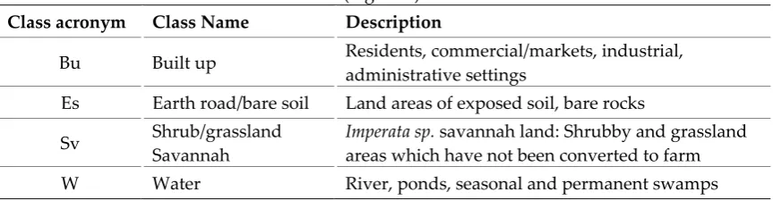
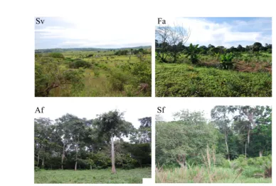
Table 2. Description of the thematic land cover types used for classification of land cover
196
(Figure 2).
197
Class acronym Class Name Description
Bu Built up Residents, commercial/markets, industrial, administrative settings
Es Earth road/bare soil Land areas of exposed soil, bare rocks
Sv Shrub/grassland Savannah
Af Perennial cocoa agroforests
Land areas used for cocoa production with various degrees of canopy stratification: canopy/shade trees are mainly deciduous
Fa
Subsistence farming
Savannah and forest land areas that have been converted essentially for permanent or seasonal subsistence crop production; including farm fallows
Sf Transition/Secondary forest
Disturbed and gallery forest patches, secret/cultural forest, hunting forest: have a more permanent and less stratified canopy structure
198
199
200
201
202
Figure 2. The range of vegetation land cover differ mainly in the density of woody biomass,
203
which changes with season or phenological period. Class acronyms are described in Table 2.
204
205
3.3 Image processing workflow
206
For RapidEye images, the following pre-processing protocol was conducted: atmospheric
207
rectification by dark object subtraction (DOS), radiometric calibration to reflectance values, geometric
208
correction, and finally computing different vegetation indices from a mosaicked image. After
209
subsetting the SAR images, we used the batch processing mode of SNAP for the following
pre-210
processing steps: radiometric calibration to Sigma0 (decibels), and geocoding with SRTM 3sec DEM
211
using RangeDoppler Terrain Correction. We used intensity backscatter profile (Figure 3) and the
212
Random Forest (RF) important variables criterion to remove noisy SAR images, and selected a
213
subsample of 10 (of the 50) important images that represent six wet and four dry seasons between
214
2015 and 2017 (see summary description in Table 1 and Figure 4).
215
The image processing steps, detailed in following subsections, comprised of three major
216
categories: (a) Feature extraction: this consisted of computing images of vegetation indices and
217
GLCM texture images; (b) Image classification: we co-registered the vegetation index and texture
218
images into the separate stacks or models described in Table 3. Then we ran eight RF ensemble
219
(machine learning) classification algorithms, using the image stacks as input (Table 3), and (c)
Post-220
processing: estimation of uncertainties in classified maps, in addition to accuracy metrics, as the basis
221
accuracy, we evaluated GLCM texture images at four different grey level quantization, to improve
223
classification uncertainties.
224
225
226
227
228
229
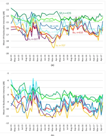
Figure 3. Radar backscatter intensity temporal profiles for the different land use/cover types
230
using the SAR images. (a) Vertical transmitted, horizontal receive backscatter; (b) Vertical
231
transmitted, vertical received backscatter. The number, n, for each label pertains to the amount of the
232
sample pixels (10×10m2)
235
236
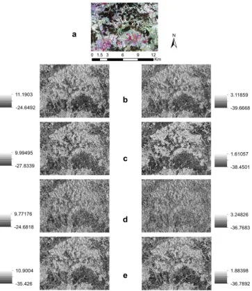
Figure 4. Radar backscatter intensity (dB) images of study landscape for key seasons from 2015
237
to 2017. (a) RapidEye false colour (RGB: bands 1, 2, and 3) composite image; (b) start of wet season:
238
17 August, 2015; (c) peak dry season: 20 March, 2016; (d) peak wet season: 4 September, 2016; (e) mid
239
of dry season: 14 January, 2017. The left and right columns are, respectively, the VV and VH
240
backscatter for each image. The North and scale bar is applicable to all images.
241
242
3.3.1. Feature extraction: Vegetation Indices (VIs) and GLCM texture features
243
The monitoring of vegetation status and extent is often based on normalisation ratios of spectral
244
bands, in the Visible and Near Infrared (NIR) spectrum [42] in spaceborne imagery. These ratios are
245
based on the contrasting spectral response of vegetation to the Red and NIR wavelengths.
246
The application of indices such as NDVI (Normalised Difference Vegetation Index) for
247
vegetation monitoring have faced several challenges [43], notably issue of saturation for biomass
248
above certain thresholds, and which is common in moist tropical vegetation. And, although
249
saturation may not be an issue over agricultural landscapes, reflectance from soil background often
250
perturb discrimination of sparse vegetation or cropland from bare soil [44]. In this study, we used
251
VIs whose values indicate the status and abundance of vegetation and biomass, and that minimise
252
the effect of soil background on vegetation reflectance values [45]: NDVI, gNDVI (green NDVI), EVI2
253
(Enhanced Vegetation Index), SAVI (Soil Adjusted Vegetation Index), and MSAVI (Modified SAVI)
254
optical sensors include an additional spectral band - the red edge band featured in RapidEye and
256
Sentinel2 [51]. This band is located between red absorption (by chlorophylls) zone, and the NIR
257
waveband.Since radar backscatter signals from a ground resolution cell are pseudorandom, the
258
interaction of microwaves with terrain objects may be difficult to predict. Moreover, SAR images
259
have speckle effect because the response signal of a resolution cell is a coherent interference from
260
multiple scattering elements within the cell. Based on texture information extraction, the analysis of
261
SAR images has been used for discrimination of cropland [26] and forest biomass estimation [27].
262
Often, the GLCM statistical approach is used in analysing SAR textures. The GLCM is a sparse matrix
263
that stores co-occurrence probabilities of inter-pixel grey levels in an image [33]. These probabilities
264
provide a second-order measure for texture features in an image: they represent conditional joint
265
probabilities of all pairwise combination of grey levels (G) in the spatial window of analysis, and
266
depend on both the spatial orientation (θ) and displacement distance (δ). Computation of GLCM is
267
faster for images with fewer grey levels, because the matrix is dimensioned to G. The conditional
268
probabilities are estimated as follows:
269
270
Pr(𝑥) = 𝐶 (𝜃, 𝛿) (1)
271
Where, Cij = co-occurrence probability between grey level i and j; and is defined by
272
273
𝐶 = 𝑃 ∑⁄ , 𝑃 (2)
274
Where, Pij = number of occurrence of grey levels i and j within the given window, for a certain
275
(θ, δ) pair; G = the quantized number of grey levels. The denominator sums up to the total number
276
of grey level pairs (i, j) within the analysis window.
277
278
Although different second-order statistics are commonly used to classify single images [52],
279
some GLCM texture measures are auto-correlated [33]: a selection of a few texture measures may be
280
reliable in achieving specific image analysis objective(s) [32]. We assess the accuracy of SAR images,
281
covering several seasons, in discriminating perennial agroforestry land cover, using four less
282
correlated GLCM texture measures: Contrast, Entropy,Correlation, and Variance. We estimated the
283
textures measures from GLCM using a 5×5 moving window, an aggregate orientation of four
284
directions (0°, 45°, 90°, and 135°), and one-pixel displacement (inter-pixel distance).
285
286
𝐶𝑜𝑛𝑡𝑟𝑎𝑠𝑡 = ∑ ∑ 𝑃, (𝑖 − 𝑗) (4)
287
288
𝐸𝑛𝑡𝑟𝑜𝑝𝑦 = ∑ ∑ 𝑃, log 𝑃, (5)
289
290
𝑉𝑎𝑟𝑖𝑎𝑛𝑐𝑒 = 𝜎 = ∑, 𝑃, (𝑖 − 𝜇 ) (6)
291
292
𝐶𝑜𝑟𝑟𝑒𝑙𝑎𝑡𝑖𝑜𝑛 = ∑ 𝑃,
( )
, (7)
293
294
where Pi,j is the joint probability distribution of the grey levels i and j at two ends of a displacement
295
vector in the assessment window, and G is the number of rows or columns. Since we considered a
296
symmetrical GLCM, 𝜇 ≡ 𝜇 𝑎𝑛𝑑 𝜎 ≡ 𝜎 . And for Entropy, 0 × ln(0) = 0 , since ln(0) is undefined.
297
298
3.3.2. Classification: Random Forest ensemble algorithm
299
In this study, we used a non-parametric machine learning algorithm, the Random Forest (RF)
300
ensemble as an image classifier. This algorithm builds multiple decision trees for the same dataset
301
based on random bootstrapping of sample training data [53] . The random forest classifier is less
302
influenced by the common issue of over-fitting and is able to handle a large number of variables [54].
303
Firstly, each tree is built from a random subset (n) of two thirds of the original samples (N) – the
‘in-304
dataset – mtry, in each decision tree nodes are split using a best split variable – the one that yields the
306
highest decrease in impurity [54]. The algorithm is a soft classifier on the basis of the probability
307
voting of pixels belonging into the respective classes considered (Table 2). Compared to other
non-308
parametric classification algorithms, it is less constrained by the need of extensive training and test
309
data samples; this is due to an integrated out-of-bag (OOB) error estimation and accuracy test
310
following a bootstrap sub-sampling on input data. Several sources provide additional details on the
311
random forest algorithm [54,55].
312
We ran eight RF models for the different images stacks as classifier input (Table 3). For each
313
model, we evaluated the OOB error curve and mtry to prune decision trees to an optimal number.
314
For a spatially explicit and unbiased representation of each land cover class in the RF models, we
315
divided the extracted pixel information for each class into a stratified random sample of 70% and 30%
316
pixels respectively for training and testing the models. Image classification was conducted using the
317
random forest package [56] of R programming software 3.4.3.
318
319
Table 3. The respective image stacks, used to compare the Random Forest (RF) classification
320
accuracy.
321
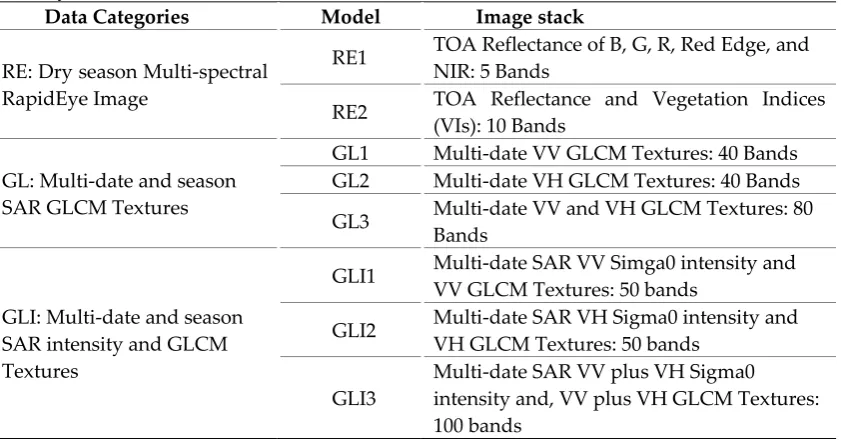
Data Categories Model Image stack
RE: Dry season Multi-spectral RapidEye Image
RE1 TOA Reflectance of B, G, R, Red Edge, and NIR: 5 Bands
RE2 TOA Reflectance and Vegetation Indices (VIs): 10 Bands
GL: Multi-date and season SAR GLCM Textures
GL1 Multi-date VV GLCM Textures: 40 Bands GL2 Multi-date VH GLCM Textures: 40 Bands
GL3 Multi-date VV and VH GLCM Textures: 80 Bands
GLI: Multi-date and season SAR intensity and GLCM Textures
GLI1 Multi-date SAR VV Simga0 intensity and VV GLCM Textures: 50 bands
GLI2 Multi-date SAR VH Sigma0 intensity and VH GLCM Textures: 50 bands
GLI3
Multi-date SAR VV plus VH Sigma0 intensity and, VV plus VH GLCM Textures: 100 bands
322
Several studies have used RF for classification of forest cover [57] and cropland [26]. Although
323
data over-fitting and poor prediction with RF approach has been reported [58] contrarily, it has been
324
shown to provide relatively better classification of croplands [26] and mangrove vegetation [52]. Thus
325
the performance of the RF ensemble classification algorithm may vary for different landscapes and
326
cropping systems. For example, Loosvelt et al. [59], observed a high classification uncertainties for
327
mixed pixels, at the heterogeneous boundaries of internally homogeneous cropping fields. Likewise,
328
Van Tricht et al. [60], reported low classification confidence at such crop boundaries. Mixed
329
cropping systems are common and the norm in moist tropical landscapes. However, reported
330
research on the processing and use of SAR images for mapping of tropical heterogeneous cropping
331
land, such as perennial agroforestry, is scarce.
332
333
3.3.3 . Post-processing and classification uncertainty assessment
334
In remote sensing mapping, the validity and reliability of classified maps are often decided on
335
basis of estimated overall accuracy and kappa coefficient [26]. Values such as user’s and producer’s
336
accuracy are prone to errors and uncertainties [61]. As a soft classifier, however, the RF algorithm
337
provides the possibility for assessing data- and computation-related uncertainties [59]. In our
338
analysis, we used user’s accuracy (omission error), producer’s accuracy (commission error), overall
339
accuracy. However, the pixel-based classification methods are prone to uncertainties coming from
341
either the use of unreliable data [61]. Thus, RF algorithm, as a soft classifier, provides a vector (Pu) of
342
classification probability or votes for each image pixel - Pu= P1, P2, P3,……, Pn for a classification with
343
n categories, and Pi denotes the probability of belonging to class i (Table 2).
344
In this study, in addition to model OOB error estimation, we evaluated classification
345
uncertainties of RF models using the maximum classifier probability (U), and a weighted uncertainty
346
measure entropy: the Shannon entropy (H) (Shannon, 1948; Vajapeyam, 2014). These uncertainties
347
were calculated as:
348
𝑈 = 1 − 𝑃 (8)
349
𝐻 = − ∑ 𝑃 . log 𝑃 (9)
350
351
Where, Pi = probability of belonging to class i and Pmax = maximum probability vote for a pixel’s
352
class. N = the total number of classes considered for analysis.
353
The maximum probability class assignment, by the soft classifier, for a pixel does not always
354
result in assigning the true class label to the concerned pixel. Thus, by considering the entire range of
355
values in a pixel’s probability vector, H, compared to U that only makes use of Pmax, provides a more
356
robust measure of uncertainty; it has a maximum value at highest entropy – equal probability votes
357
for all classes considered.
358
Loosvelt et al. [59], showed that H is reliable for evaluating uncertainties in mapping cropland
359
from SAR images. However, our study area is characterised by heterogeneous cropping systems and
360
is located in a tropical landscape (Figure 2). For the best-performing RF models, based on kappa
361
accuracy, we computed and analysed U and H uncertainties for the classified maps, and the land
362
cover classes considered in the study area (Table 2). The uncertainty estimations and analysis were
363
conducted in Spyder IDE (Integrated Development Environment) of Anaconda distribution for
364
Python programming software version 3.0 (Anaconda 3)
365
366
367
Figure 5. Schematic outline of the image processing and texture feature extraction, and land
370
use/cover (LCLU) delineation by a machine learning algorithm. Input and outputs are shaded, and
371
feature extraction in broken border lines. DOS: Dark object subtraction, TOA: Top of Atmosphere
372
373
4. Results
374
All the RF models had classification accuracies above 70%. Classification error and the
375
sensitivity in discriminating land cover classes was different for each model. The models with the
376
highest classification reliability, in increasing order of importance, were RE1, GLI3, and GL3.
377
4.1 Classification accuracy
378
Table 4 summarizes the classification results for all eight RF models. All models had a reliable
379
overall accuracy (OA) above 70%. However, compared to using VV or VH bands separately, the use
380
of both co- and cross-polarization bands (GL3) resulted in the highest classification accuracy. The
381
GL3 model had the highest overall accuracy of 88.1% and kappa of 0.85; and, compared to other
382
models, the OOB error estimate was the least with 12.8%. Also, classification from the multi-spectral
383
optical image (RE1 model) had a reliable overall accuracy of 81.1%, but it had a lower kappa 76.9%.
384
Compared to the GL3 model, the OOB error difference of +7% was observed for the RE1. The GLCM
385
textures are reliable for discriminating the land cover/uses. And considering the heterogeneous and
386
dynamic vegetation in the landscape, an improvement feature selection using the GLCM approach is
387
necessary to reduce class uncertainties.
388
389
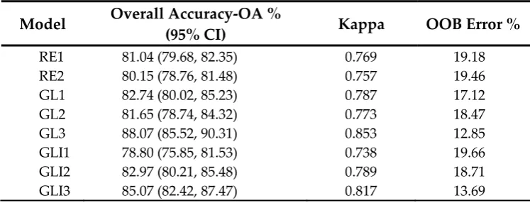
Table 4. Classification accuracies of different feature models based on the Random Forest (RF)
390
classifier algorithm.
391
392
Model Overall Accuracy-OA %
(95% CI) Kappa OOB Error %
RE1 81.04 (79.68, 82.35) 0.769 19.18
RE2 80.15 (78.76, 81.48) 0.757 19.46
GL1 82.74 (80.02, 85.23) 0.787 17.12
GL2 81.65 (78.74, 84.32) 0.773 18.47
GL3 88.07 (85.52, 90.31) 0.853 12.85
GLI1 78.80 (75.85, 81.53) 0.738 19.66
GLI2 82.97 (80.21, 85.48) 0.789 18.71
GLI3 85.07 (82.42, 87.47) 0.817 13.69
393
The thematic land cover map from RE1 and GL3 models are shown in Figure 6. Separately, both
394
VV and VH GLCM derived texture measures were poor in the prediction of non-vegetated land
395
covers, and more so when both bands were included in the same model (Figure 6b). When included
396
as input layers, the SAR backscatter intensity did not improve classification accuracy. Likewise, the
397
inclusion of vegetation indices from the multispectral optical image, taken during a dry season, did
398
not improve classification accuracy (Figure 6a). The texture measures from both VH and VH
399
backscatter provide comparable, and may be complementary, LULC mapping accuracy to the
400
commonly used vegetation indices of optical image.
401
403
404
Figure 6. Pixel-based classification result for the eight models evaluated by random forest
405
ensemble algorithm. (a) Classification accuracy; (b) Class reliability estimates; (c) Thematic land
406
cover/use map from model RE1; (d) Thematic map model GL3. The scale, legend and north arrow
407
apply to both c and d.
408
409
Visually, RE1 map shows a relatively intact and continuous expanse of transition forest patches
410
(Figure 6c). Contrarily, the classified map from GL3 revealed that transition forest cover is highly
411
fragmented by cocoa agroforests into smaller patches (Figure 6d). Also, from classification
412
reliability estimates (100 - commission error) in Figure 6b, the RE1 model was more reliable in
413
delineating non-vegetation land features. SAR-based texture images had a high reliability in
414
delineating vegetation landscape features (Sv, Af, Fa, and Sf). Thus, although multi-spectral optical
415
image had a better classification prediction of land cover classes in general, it was less reliable in
416
discriminating perennial agroforests from transition forest land cover.
417
4.2 Uncertainty in discriminating vegetation land cover
418
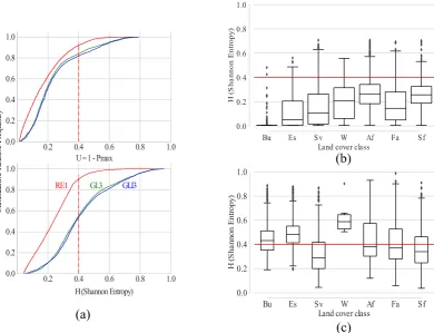
The classification results from dry season RapidEye multi-spectral optical image (RE1) had a low
419
overall and class uncertainties. From the cumulative estimates of class probabilities in Figure 7,
420
classification uncertainty from the RE1 converges at a probability of around 0.6 for both U and H,
421
whereas the uncertainty from GL3 map converges at higher probabilities – 0.7 and 0.9 respectively
422
for U and H (Figure 7a). About 90% of pixels classified by RE1 had H uncertainties below 0.4,
423
compared to about 50% of pixels for GL3. This difference is less obvious in the cumulative plot of U.
424
Thus, uncertainty difference between RE1 and Gl3 was better revealed by Shannon entropy or H
425
uncertainty.
426
428
429
Figure 7. Classification uncertainties as validation of models with highest accuracy. (a) The
430
Shannon entropy (H) clearly reveals uncertainty in classification accuracy validation. For the thematic
431
maps from RE1 and GL3 R models: As example, the proportion of pixels with uncertainty below 0.4;
432
(b) Individual class uncertainty, (H), for model RE1; (c) Class uncertainty, (H), for model GL3.
433
434
The individual class uncertainties are compared in Figure 7. Although the classified map from
435
the multi-spectral image (RE1 model) had a lower accuracy, the class uncertainty was, compared to
436
other land cover types, high for perennial cocoa agroforests and transition forest cover (Figure 7b).
437
In comparison to RE1, the multi-seasonal SAR image textures, from the GL3 model, had a high overall
438
uncertainty of a pixel’s class prediction. However, perennial agroforests and transition forests were
439
discriminated with relatively lower individual class uncertainty (Figure 7c): The median of class
440
uncertainties were in a range between 0.2 and 0.4, which is comparable to those obtained from the
441
single date multi-spectral image (RE1). The uncertainties in land cover/use discrimination by RE1
442
may reflect vegetation status/phenology - canopy greenness; while, in the GL3 model, volume
443
scattering of radar signal reflects changes in water content and structure in different vegetation
444
canopy.
445
4.3 Contribution of pixel depth to texture feature extraction
446
The SAR backscatter intensity images have a pixel quantization of 32 bits. The likelihood of grey
447
level co-occurrences was lower at such high dynamic pixel range, as observable from unclassified
448
pixels, Un class, in Figure 6c. In order to improve classification uncertainty from SAR image textures,
449
we computed and compared three (3) different image pixel quantization or grey levels; 32bits – GL3
450
(as in original SAR intensity image), 8bits – GL3_B8, 6bits – GL3_B6, and 4bits – GL3_B4.
451
The contribution of grey levels on GLCM feature co-occurrence and classification probability is
452
shown in Figure 8 and Table 5. Pixel co-occurrence was low at high pixel dynamic ranges (Figure
453
8a), which resulted in a large clustering of features with low and no predictions in Figures 8a and d.
454
The dynamic pixel range of 64 grey level significantly reduced the prediction error (Figure 8e). The
455
class prediction probability is improved to a maximum of 0.99 in GL3_B6, with a difference of 7%
456
bits (Figure 8d). Optimizing the image pixel depth resulted in a marginal improvement of
458
classification accuracy to a kappa value of 86.22 (Table 5). Though, the OOB error of prediction is
459
reduced remarkably from the initial 12.8% (GL3) to 9.9% in GL3_B6. These results show that the
460
dynamic pixel range was vital in feature selection (co-occurrence between pixels), and texture feature
461
extraction by the ensemble algorithm.
462
463
464
465
Figure 8. Classification probability maps reveal improved pixel classification with at lower grey
466
level quantization. (a) Co-occurrence values in the first 5 × 5 cells of GLCM; (b) Sample details of the
467
four GLCM texture measures; (c) to (f) are snips showing the respective details of the classification
468
probability map for GL3, GL3_B8, GL3_B6, and GL3_B4 models. Unclassified areas are shown as red
469
pixels in (c) and (d)
470
471
Table 5. Classification results of different grey level GLCM models and land cover/use surface
472
area estimates. See Appendix A for details of class errors.
473
Model Overall Accuracy-OA %
(95% CI) Kappa
OOB Error %
RE1 81.04 (79.68, 82.35) 0.769 19.18
GL3 88.07 (85.52, 90.31) 0.854 12.85
GL3_B8 88.23 (85.74, 90.41) 0.854 11.84 GL3_B6 88.83 (86.48, 90.90) 0.862 9.92 GL3_B4 88.86 (86.50, 90.94) 0.862 10.38
474
The improvements in the predicted land cover/use maps, after optimizing the dynamic pixel
475
ranges, are illustrated in Figures 9 and 10. Figure 9 shows the predicted maps for the different
texture-476
based models. Compared to the classification from GL3, at 32 bits pixel depth, with an estimated
477
647.3 ha as unclassified area (Figure 9a), the analysis at 6bits dynamic pixel range show less mosaic
478
in discriminating class areas and reduced the unclassified land area to about 7.4 ha (Figure 9c). See
479
The model validation results, by Shannon Entropy estimates, are shown in Figure 10. The difference
481
in class uncertainty between GL3 and GL3_B6 is most evident for the following classes; Built up (Bu),
482
Cocoa agroforests (Af), subsistence farms (Fa), and transition forests (Sf). The GL3_B6 had a
483
comparable lower class error for these classes: respectively 16.4%, 4.4%, 5.3%, and 6.1% (see Figure
484
A1 in Appendix). Remarkably, the class uncertainty estimates for Sf is low and comparable for
485
GL3_B6 and RE1. Unlike the RE1 model, with no difference in class uncertainty between Af and Sf,
486
the significant distinction between their class uncertainties in the GL3_B6 confirms the reliability of
487
the model to discriminate these two vegetation categories.
488
489
490
Figure 9. Classification prediction, based on Random forest algorithm, for the GLCM
texture-491
based models. (a) GL3; (b) GL3_B8; (c) GL3_B6; (d) GL3_B4; (e) to (h) are corresponding details of the
492
prediction maps in area 1 ; (i) to (l) are corresponding details in area 2. The legend and north arrow
493
apply to all images and the scale bar to images (e) to (l).
494
495
496
497
Figure 10. Comparison of validation by Shannon Entropy (H) estimation. Class uncertainty estimate
498
is significantly improve by the GL3_B6, as observed for Built-up areas (Bu), Cocoa agroforests (Af),
499
subsistence farmlands (Fa) and transition forests (Fs).
500
501
2
1 1
2 2
1 1
2
±
0 0.5 1 2 3 4
Km
(a) (b) (c) (d)
(e) (f) (g) (h)
(i) (j) (k) (l)
The estimated land cover/use against the reference model (RE1) is shown in Figure 11. The total
502
area for each class is summarized in Table A3 (see Appendix). A signification reduction in
503
unclassified area is shown in 11c and d. The area of transition forest is lower for all models than
504
estimated by RE1. Though the class error and uncertainty for GL3_B6 is comparable to that of RE1
505
(Figure 10). The land area for subsistence farming, cocoa agroforests and built up is remarkably larger
506
in the texture-based predicted maps.
507
508
509
Figure 11. Comparison of the predicted land cover/use from RE1 model (optical image), in the
510
landscape surface area of 11344.61ha, with: (a) GL3; (b) GL3_B8; (c) GLC_B6; and (d) GL3_B4. See
511
Table A2.
512
5. Discussion
513
Land use and land cover (LULC) classification of satellite image is commonly applied to
mono-514
date images; we use a rapidEye image that was acquired in the dry season – during minimal or no
515
hindrance from cloud cover. In LULC change detection, a temporal series of images is often used,
516
which require a reliable consistency in the characteristics of the processed images. For SAR image
517
processing, therefore, image filtering or multi-looking is often applied to reduce speckle noise in SAR
518
images [60]. However, such pre-processing also reduces the resolution of images. Thus, considering
519
the landscape structure and the inherently heterogeneous vegetation categories in this study, we did
520
not considered image speckle as noise. The selected SAR images were recorded during the ascending
521
satellite overpass. We conducted a temporal average of measured textures across seasons, which,
522
reduced any potential noise from individual image pixels; meanwhile, the seasonal differences in
523
volume scattering over vegetation cover provided the texture details for discriminating the
524
vegetation types. The temporal SAR data and the texture measures were, however, less sensitive to
525
mapping non-vegetation land cover - notably the water cover. The low classification sensitivity for
526
water areas can be explained by the following: variability in water cover as a result of seasonal
527
swampy areas, the seasonal conversion of some swampy areas into subsistence farms of adapted
528
in the GLCM. Consequently, the GLCM had a low likelihood to extract texture for the water class.
530
Nonetheless, this land cover was not of main interest in this study.
531
Compared to a “business as usual” classification using a mono-season multi-spectral optical
532
image (RE1), a combination of texture from both VV and VH bands and the 6bits grey level
533
quantization prior to GLCM texture classification had the highest OA of 88.1% and kappa of 0.85.
534
Moreover, this accuracy resulted in, respectively, 3% and 9.3% reduction in prediction error over the
535
GLCM texture at the default 32bits grey levels and the optical-image. Albeit the relatively low high
536
prediction error of the RE1 model, the class prediction error was low for land cover with no- and
low-537
vegetation: built up, bare soil, savannah and subsistence farmlands; these have rather distinctive
538
optical spectral signatures. For the vegetation cover with high canopy, Table A1 shows the high
539
confusion between cocoa agroforests and transition forests, both of which have high canopy. Since
540
their canopy structure is similar [16], they may not be reliably discriminated using their spectral
541
signatures [17], and less so during the dry season - of low leaf proliferation. Therefore, the
542
classification performance from optical data is logical, and for the vegetation classes, reflects the
543
vegetation status per season and phonological cycle; consequently, the optical reflectance in the dry
544
season was less distinctive for cocoa agroforests versus secondary forests.
545
In the texture-based classification, we averaged volume scattering across seasons, which
546
captured differences the vegetation types. As seen in Table A2, the confusion between cocoa
547
agroforests and transition forest is low, compared to other classes. This indicates that optimizing the
548
grey level improved the classification and helped to distinguish especially the vegetation classes with
549
high heterogeneous canopy. For the study landscape the range of backscatter intensity, for VH and
550
VV bands, is on average above 34 dB. The 6bits grey level quantization was consistent with the range
551
of backscatter intensity in both VV and VH bands, and our results on grey level quantization confirms
552
other reports [39–41]. Therefore, our land cover/use classification performance at grey level
553
quantization of 6bits or 64 levels (GL3_B6) were optimal for discriminating different vegetation,
554
particularly those featuring a high canopy. Other studies on heterogeneous cropland mapping
555
recorded an accuracy of 71% using C-band SAR intensity images [26]. However, in terms of OA, our
556
result is in line with the accuracy observed in different heterogeneous cropping landscapes using a
557
combination of C-band SAR and optical data though [26,34]. The authors [26,34], mapped cropping
558
lands with inherent homogeneous canopy. The landscape in the study is, however, tropical and
559
dominated by vegetation and cropping fields with internally heterogeneous canopy.
560
Our texture-based classification result shows spatial fragmentation of forest cover by cocoa
561
agroforests land use. These transition forest patches are consistent with field observations; the
562
transition forest patches are mostly owned by families and community groups for hunting,
563
performing traditional rituals, and serve as potential cocoa agroforests parcels. The similarity in
564
canopy structure of cocoa agroforests and transition forests is explained by their matching class
565
uncertainty estimates from the optical data i.e. RE1 model. Moreover, the confusion matrix in Table
566
A1 reveals a high commission error between the two classes. Thus, by averaging the seasonal radar
567
volume scattering, the GL3_B6 model discriminated the two vegetation cover with significantly
568
different class uncertainties: the mean class uncertainty for transition forests was 0.28 in GL3_B6
569
based on GL3_B6 model, and unlike in RE1 model, this was significantly different from the 0.4 class
570
average for cocoa agroforests. Following the high overall accuracy and a corresponding low
571
individual class uncertainty, the multi-date texture information from SAR images provided a reliable
572
classifier input for discriminating of perennial agroforestry land cover from transition forest.
573
Classification validation based on accuracy metrics as overall, user, and producer accuracies are
574
influenced by sample class distribution in training data [64]. The differences in pixel resolution
575
between images types (5 m for RapidEye and 10 m for SAR C-Band) resulted in a different number
576
of reference pixels; of which lower numbers result in low estimates of misclassification probability
577
(commission or omission errors). This explains the high overall accuracy for SAR image. The sample
578
size is not as influential in classification validation by estimates of entropy or uncertainty. Entropy is
579
a classic metric for biodiversity in ecology; thus, for this study, it describes the likelihood of a pixel
580
however, our results contradict other reported uncertainty in croplands mapping [59]; the trend of U
582
and H uncertainties were different for our study landscape. At the uncertainty of 0.4 for example, the
583
entropy or H, compared to U, revealed better the difference in the cumulative proportion of pixels
584
between RE1 and GLE models. The slope of cumulative Shannon entropy (H) was linear for RE1 and
585
sigmoidal for GL3. The former reflects a high likelihood of a single land cover class for each pixel in
586
the multi-spectral image. The sigmoid curve represents a complete range of probabilities for each
587
image pixel- a soft boundary between land cover classes. Compared to perennial agroforests, the low
588
individual class uncertainty for transition forest is logical and consistent, as there is a high temporal
589
stability of radar volume scattering over forest area [31].
590
The classification uncertainty, measured by Shannon entropy (H), for transition forests was
591
comparable for both RE1 and GL3_B6: the likelihood of a pixel being classified only as transition
592
forest was similar for both RE1 and GL3_B6 models. Noteworthy is the quantization level used for
593
GLCM computation in the later, which it reduces unclassified areas to only 7.4 ha. Consequently, the
594
forest area, estimated to cover 1706.9 ha (mean H = 0.25, class error = 0.32) using the RE1, was 500 ha
595
(mean H = 0.28, class error = 0.06) less following the estimates from GL3_B6. Although the uncertainty
596
for cocoa agroforests was significantly reduced by the GL3_B6, their relatively high entropy (mean
597
H = 0.40, class error) indicate a high likelihood of classifying cocoa agroforests as one of the other
598
classes. This distinction between the average entropy for cocoa agroforest (Af) and transition forest
599
(Sf) for GL3_B6 model, confirms a reliable discrimination of the two vegetation types. The high
600
variability in tree density and structure between cocoa agroforests may result in high intra-class
601
variations in SAR backscatter intensity and confusion with other vegetation types, which might
602
explain their high H uncertainty. Likewise, the diversity in farm subsistence crop types and stages
603
may explain the high H for the class. As well for savannah lands, there is a frequent change of canopy
604
volume and structure along with seasonal phonological cycles, except for areas converted to
605
subsistence farming or previous farms that have been left fallow. Such physical changes results to
606
unavoidable classification confusions [60]. The high class uncertainties validate the variability within
607
land cover types and land use dynamics in the landscape; therefore, the uncertainties may not be
608
easily reduced in a texture-based classification of SAR data.
609
The results of this study provide a new insight into the application of GLCM for SAR image
610
processing for mapping tropical croplands of heterogeneous and multi-strata canopy. We highlight
611
the important consideration of grey level quantization in heterogeneous land cover/use classification.
612
Depending on the landscape structure and vegetation types, though, application of SAR imagery for
613
cropland mapping may warrant different analysis procedure [26,34,60]. Thus there may be a need to
614
customised analysis parameter depending on objective and landscape characteristics. The texture
615
measures were pre-selected following the recommendation in reference [32], which is based on
616
inference from optical image classification results, are tailored for vegetation mapping. This
pre-617
selection of texture feature introduced bias in discriminating areas without vegetation. The GLCM
618
texture measures were tailored to discriminate vegetation types, and less sensitive to non-vegetation
619
cover. Texture feature extraction procedure are well established in the literature, with varying
620
opinions. We highlight here, some issues which limit this study. We estimated the GLCM textures
621
using a 5 × 5 window scale, considering the 10m pixel resolution for sentinel1 SAR. However,
622
different window sizes may influence both texture values and classification accuracy. The analysis of
623
different window sizes was not the aim of this study and may be a subject for further investigated
624
for this and other landscapes. We perceive that a fusion of texture information with optical images
625
[26,34], at a temporal scale may improve the uncertainty in discriminating vegetation classes. Also,
626
considering the diversity of vegetation across cocoa production landscapes, the complex structure
627
and canopy of cocoa agroforests, the continuous archive and improvement in SAR image resolution
628
can train deep learning procedures for land cover/use classification at the scale of several landscapes.
629
6. Conclusions
630
C-band SAR for discriminating cocoa agroforest cropping land in a heterogeneous landscape. We use
632
seasonal differences in volume scattering from the dielectric (water content) status and structure of
633
vegetation canopy as a metric to discriminate vegetation types. We make the following conclusions:
634
1. For the same window size and an invariant direction, reducing the grey level quantization
635
improved classification accuracy marginally, but significantly reduced the uncertainty in
636
discriminating cocoa agroforests from other vegetation covers.
637
2. Classification validation by estimates of Shannon entropy (H) reveal subtle differences in
638
individual class prediction and provide reliable information for making inferences in
639
heterogeneous landscape mapping.
640
3. The magnitude of forest fragmentation by cocoa agroforest, which is concealed by vegetation
641
indices from spectral reflectance, is mapped using GLCM texture measures from C-band SAR
642
images.
643
We suggest an approach for mapping cocoa agroforests in tropical heterogeneous cropping
644
landscapes using C-band SAR imagery. The approach shows the reliability of Sentinel1 SAR image
645
archive in landscape monitoring; especially for mapping cocoa agroforests expansion, and their
646
contribution to the loss of transition and primary forest cover. Therefore, it has potential application
647
in, for example, estimating the contribution of agroforestry to national and regional REDD+
648
(Reducing Emission from Deforestation and Forest Degradation and the role of conservation,
649
sustainable management of forests and enhancement of carbon stocks in developing countries)
650
strategies. However, there is a need to assess classification uncertainties in different agroforestry
651
dominant landscapes – for an operational regional mapping in the Congo Basin sub-region.
652
653
Author Contributions: Conceptualization and design of the study, Frederick N. Numbisi; methodology,
654
Frederick N. Numbisi and Frieke M.B. Van Coillie; field investigation, Frederick N. Numbisi; data curation,
655
Frederick N. Numbisi; data analysis, Frederick N. Numbisi; original draft preparation, Frederick N. Numbisi.;
656
review and editing, Frederick N. Numbisi, Frieke M.B. Van Coillie and Robert De Wulf; supervision, Frieke M.B.
657
Van Coillie and Robert De Wulf.
658
Funding: Special Research Fund, Ghent University, contract number BOF DOS01W03314
659
Acknowledgments: This study was conducted under the Special Research Fund, of Ghent University, for
660
students from developing countries, and through which RapidEye image was procured. Fieldwork was
661
supported by the World Agroforestry Centre in Cameroon. Field inventory was assisted by local resource
662
persons, administrative personnel and cocoa farmers who granted access to their plantations. We thank the
663
European Space Agency for providing the freely accessible archive of Sentinel-1 SAR imagery under the
664
Copernicus Open Data Hub. We express gratitude to developers and contributors to both R and Python
665
programming and data mining software, which are open source and free. The authors would like to thank the
666
editors of the ISPRS midterm Symposium and the anonymous reviewers for their valuable comments.
667
Conflicts of Interest: The authors declare no conflict of interest.
668
669
Appendix A
670
Table A1. Classification confusion matrix of RE1 Model. OA = Overall Accuracy, UA = User
671
Accuracy, PA = Producer Accuracy.
672
nTrees = 250, mTry = 2, OOB error = 19.2%, OA = 81.0%
Reference
Class Error PA
Bu Es Sv W Af Fa Sf
Predicted
Bu 1238 0 0 0 0 1 0 0.001 99.9
Es 2 529 8 0 0 117 0 0.194 80.6
Sv 0 0 1469 1 52 172 2 0.134 86.6
Af 0 0 64 8 855 31 335 0.339 66.1
Fa 0 57 233 0 55 1447 3 0.194 80.6
Sf 0 0 3 0 309 4 665 0.322 67.7
UA 99.8 90.3 82.3 85 66.4 81.7 66.0
673
Table A2. Classification confusion matrix of GL3_B6 Model.
674
nTrees = 550, mTry = 8, OOB error = 9.9%, OA = 88.8%
Reference
Class Error PA
Bu Es Sv W Af Fa Sf
Predicted
Bu 244 2 5 0 23 17 1 0.164 83.6
Es 14 89 19 0 6 21 0 0.403 59.7
Sv 0 0 424 0 0 12 0 0.028 97.2
W 2 0 3 0 6 7 0 1.000 0
Af 3 0 0 0 325 8 4 0.044 95.6
Fa 1 0 18 0 3 415 1 0.053 94.8
Sf 0 0 0 0 16 0 246 0.061 93.9
UA 92.4 97.8 90.4 0 85.8 86.5 97.6
675
Table A3. Predicted surface area (ha) of land cover/use for optical multi-spectral image and GLCM
676
textures at four different grey level quantization
677
LULC Class Model
RE1 Gl3 Gl3_B8 Gl3_B6 Gl3_B4
Bu 68.89 547.38 650.35 545.89 719.07
Es 160.73 73.41 235.14 83.14 76.15
Sv 4485.2 3118.63 3035.37 3465.95 3629.72
W 137.08 0.27274 0.15079 0.16927 0.16446
Af 2733.63 2986.84 2904.18 3355.87 3254.77
Fa 2052.11 2787.95 3081.47 3120.90 3002.42
Sf 1706.94 1202.86 1306.70 1210.16 1094.61
Un 0 647.32 562.62 7.42 12.60
678
References
679
1. FAO. 2016. State of the World’s Forests 2016. Forests and agriculture: land-use challenges and opportunities.
680
Rome.; 2016; ISBN 9789251092088.
681
2. Ordway, E. M.; Asner, G. P.; Lambin, E. F. Deforestation risk due to commodity crop expansion in
sub-682
Saharan Africa Deforestation risk due to commodity crop expansion in sub- Saharan Africa. Environ.
683
Res. Lett.2017, 12, doi:10.1088/1748-9326/aa6509.
684
3. Payne, O.; Mann, A. S. Zomming In:"Sustainable" Cocoa Producer Destroys Pristine Forest in Peru
685
Available online: