DOI:10.1051/0004-6361/201525898 c
ESO 2016
Astronomy
&
Astrophysics
Planck 2015 results
Special feature
Planck
2015 results
XX. Constraints on inflation
Planck Collaboration: P. A. R. Ade99, N. Aghanim66, M. Arnaud82, F. Arroja74,88, M. Ashdown78,6, J. Aumont66, C. Baccigalupi97, M. Ballardini54,56,37, A. J. Banday112,11, R. B. Barreiro73, N. Bartolo36,74, E. Battaner114,115, K. Benabed67,111, A. Benoît64, A. Benoit-Lévy28,67,111, J.-P. Bernard112,11, M. Bersanelli40,55, P. Bielewicz92,11,97, J. J. Bock75,13, A. Bonaldi76, L. Bonavera73, J. R. Bond10,
J. Borrill16,104, F. R. Bouchet67,102, F. Boulanger66, M. Bucher1,?, C. Burigana54,38,56, R. C. Butler54, E. Calabrese107, J.-F. Cardoso83,1,67, A. Catalano84,81, A. Challinor70,78,14, A. Chamballu82,18,66, R.-R. Chary63, H. C. Chiang32,7, P. R. Christensen93,43, S. Church106, D. L. Clements62, S. Colombi67,111, L. P. L. Colombo27,75, C. Combet84, D. Contreras26, F. Couchot80, A. Coulais81, B. P. Crill75,13,
A. Curto73,6,78, F. Cuttaia54, L. Danese97, R. D. Davies76, R. J. Davis76, P. de Bernardis39, A. de Rosa54,
G. de Zotti51,97, J. Delabrouille1, F.-X. Désert60, J. M. Diego73, H. Dole66,65, S. Donzelli55, O. Doré75,13, M. Douspis66, A. Ducout67,62, X. Dupac46, G. Efstathiou70, F. Elsner28,67,111, T. A. Enßlin89, H. K. Eriksen71, J. Fergusson14, F. Finelli54,56,?, O. Forni112,11, M. Frailis53,
A. A. Fraisse32, E. Franceschi54, A. Frejsel93, A. Frolov101, S. Galeotta53, S. Galli77, K. Ganga1, C. Gauthier1,88, M. Giard112,11, Y. Giraud-Héraud1, E. Gjerløw71, J. González-Nuevo23,73, K. M. Górski75,116, S. Gratton78,70, A. Gregorio41,53,59, A. Gruppuso54, J. E. Gudmundsson109,95,32, J. Hamann110,108, W. Handley78,6, F. K. Hansen71, D. Hanson90,75,10, D. L. Harrison70,78, S. Henrot-Versillé80, C. Hernández-Monteagudo15,89, D. Herranz73, S. R. Hildebrandt75,13, E. Hivon67,111, M. Hobson6, W. A. Holmes75, A. Hornstrup19, W. Hovest89, Z. Huang10, K. M. Huffenberger30, G. Hurier66, A. H. Jaffe62, T. R. Jaffe112,11, W. C. Jones32, M. Juvela31, E. Keihänen31, R. Keskitalo16, J. Kim89,
T. S. Kisner86, R. Kneissl45,8, J. Knoche89, M. Kunz20,66,3, H. Kurki-Suonio31,50, G. Lagache5,66, A. Lähteenmäki2,50, J.-M. Lamarre81, A. Lasenby6,78, M. Lattanzi38, C. R. Lawrence75, R. Leonardi9, J. Lesgourgues68,110, F. Levrier81, A. Lewis29, M. Liguori36,74, P. B. Lilje71, M. Linden-Vørnle19, M. López-Caniego46,73, P. M. Lubin34, Y.-Z. Ma26,76, J. F. Macías-Pérez84, G. Maggio53, D. Maino40,55, N. Mandolesi54,38,
A. Mangilli66,80, M. Maris53, P. G. Martin10, E. Martínez-González73, S. Masi39, S. Matarrese36,74,48, P. McGehee63, P. R. Meinhold34, A. Melchiorri39,57, L. Mendes46, A. Mennella40,55, M. Migliaccio70,78, S. Mitra61,75, M.-A. Miville-Deschênes66,10, D. Molinari73,54, A. Moneti67,
L. Montier112,11, G. Morgante54, D. Mortlock62, A. Moss100, M. Münchmeyer67, D. Munshi99, J. A. Murphy91, P. Naselsky94,44, F. Nati32, P. Natoli38,4,54, C. B. Netterfield24, H. U. Nørgaard-Nielsen19, F. Noviello76, D. Novikov87, I. Novikov93,87, C. A. Oxborrow19, F. Paci97,
L. Pagano39,57, F. Pajot66, R. Paladini63, S. Pandolfi21, D. Paoletti54,56, F. Pasian53, G. Patanchon1, T. J. Pearson13,63, H. V. Peiris28, O. Perdereau80, L. Perotto84, F. Perrotta97, V. Pettorino49, F. Piacentini39, M. Piat1, E. Pierpaoli27, D. Pietrobon75, S. Plaszczynski80, E. Pointecouteau112,11, G. Polenta4,52, L. Popa69, G. W. Pratt82, G. Prézeau13,75, S. Prunet67,111, J.-L. Puget66, J. P. Rachen25,89, W. T. Reach113,
R. Rebolo72,17,22, M. Reinecke89, M. Remazeilles76,66,1, C. Renault84, A. Renzi42,58, I. Ristorcelli112,11, G. Rocha75,13, C. Rosset1, M. Rossetti40,55, G. Roudier1,81,75, M. Rowan-Robinson62, J. A. Rubiño-Martín72,22, B. Rusholme63, M. Sandri54, D. Santos84, M. Savelainen31,50, G. Savini96, D. Scott26, M. D. Seiffert75,13, E. P. S. Shellard14, M. Shiraishi36,74, L. D. Spencer99, V. Stolyarov6,105,79, R. Stompor1, R. Sudiwala99,
R. Sunyaev89,103, D. Sutton70,78, A.-S. Suur-Uski31,50, J.-F. Sygnet67, J. A. Tauber47, L. Terenzi98,54, L. Toffolatti23,73,54, M. Tomasi40,55, M. Tristram80, T. Trombetti54, M. Tucci20, J. Tuovinen12, L. Valenziano54, J. Valiviita31,50, B. Van Tent85, P. Vielva73, F. Villa54, L. A. Wade75,
B. D. Wandelt67,111,35, I. K. Wehus75,71, M. White33, D. Yvon18, A. Zacchei53, J. P. Zibin26, and A. Zonca34 (Affiliations can be found after the references)
Received 14 February 2015/Accepted 3 March 2016
ABSTRACT
We present the implications for cosmic inflation of thePlanckmeasurements of the cosmic microwave background (CMB) anisotropies in both temperature and polarization based on the fullPlancksurvey, which includes more than twice the integration time of the nominal survey used for the 2013 release papers. ThePlanckfull mission temperature data and a first release of polarization data on large angular scales measure the spectral index of curvature perturbations to bens=0.968±0.006 and tightly constrain its scale dependence to dns/dlnk=−0.003±0.007 when combined with thePlancklensing likelihood. When thePlanckhigh-`polarization data are included, the results are consistent and uncertainties are further reduced. The upper bound on the tensor-to-scalar ratio isr0.002<0.11 (95% CL). This upper limit is consistent with theB-mode polarization constraintr<0.12 (95% CL) obtained from a joint analysis of the BICEP2/Keck Array andPlanckdata. These results imply thatV(φ)∝φ2and natural inflation are now disfavoured compared to models predicting a smaller tensor-to-scalar ratio, such asR2inflation. We search for several physically motivated deviations from a simple power-law spectrum of curvature perturbations, including those motivated by a reconstruction of the inflaton potential not relying on the slow-roll approximation. We find that such models are not preferred, either according to a Bayesian model comparison or according to a frequentist simulation-based analysis. Three independent methods reconstructing the primordial power spectrum consistently recover a featureless and smoothPR(k) over the range of scales 0.008 Mpc−1 <∼k<∼0.1 Mpc−1. At large scales, each method finds
deviations from a power law, connected to a deficit at multipoles`≈20−40 in the temperature power spectrum, but at an uncompelling statistical significance owing to the large cosmic variance present at these multipoles. By combining power spectrum and non-Gaussianity bounds, we constrain models with generalized Lagrangians, including Galileon models and axion monodromy models. ThePlanckdata are consistent with adiabatic primordial perturbations, and the estimated values for the parameters of the baseΛcold dark matter (ΛCDM) model are not significantly altered when more general initial conditions are admitted. In correlated mixed adiabatic and isocurvature models, the 95% CL upper bound for the non-adiabatic contribution to the observed CMB temperature variance is|αnon-adi|<1.9%, 4.0%, and 2.9% for CDM, neutrino density, and neutrino velocity isocurvature modes, respectively. We have tested inflationary models producing an anisotropic modulation of the primordial curvature power spectrum finding that the dipolar modulation in the CMB temperature field induced by a CDM isocurvature perturbation is not preferred at a statistically significant level. We also establish tight constraints on a possible quadrupolar modulation of the curvature perturbation. These results are consistent with thePlanck2013 analysis based on the nominal mission data and further constrain slow-roll single-field inflationary models, as expected from the increased precision ofPlanckdata using the full set of observations.
Key words. cosmic background radiation – cosmology: theory – early Universe – inflation
1. Introduction
The precise measurements byPlanck1of the cosmic microwave background (CMB) anisotropies covering the entire sky and over a broad range of scales, from the largest visible down to a reso-lution of approximately 50, provide a powerful probe of cosmic
inflation, as detailed in thePlanck2013 inflation paper (Planck Collaboration XXII 2014, hereafterPCI13). In the 2013 results, the robust detection of the departure of the scalar spectral in-dex from exact scale invariance, i.e.,ns < 1, at more than 5σ
confidence, as well as the lack of the observation of any statis-tically significant running of the spectral index, were found to be consistent with simple slow-roll models of inflation. Single-field inflationary models with a standard kinetic term were also found to be compatible with the new tight upper bounds on the primordial non-Gaussianity parameters fNL reported in Planck Collaboration XXVI (2014). No evidence of isocurva-ture perturbations as generated in multi-field inflationary mod-els (PCI13) or by cosmic strings or topological defects was found (Planck Collaboration XXV 2014). ThePlanck2013 re-sults overall favoured the simplest inflationary models. However, we noted an amplitude deficit for multipoles` <∼40 whose sta-tistical significance relative to the six-parameter base Λ cold dark matter (ΛCDM) model is only about 2σ, as well as other anomalies on large angular scales but also without compelling statistical significance (Planck Collaboration XXIII 2014). The constraint on the tensor-to-scalar ratio,r<0.12 at 95% CL, in-ferred from the temperature power spectrum alone, combined with the determination of ns, suggested models with concave
potentials.
This paper updates the implications for inflation in the light of thePlanckfull mission temperature and polarization data. The
Planck2013 cosmology results included only the nominal mis-sion, comprising the first 14 months of the data taken, and used only the temperature data. However, the full mission includes the full 29 months of scientific data taken by the cryogenically cooled high frequency instrument (HFI; which ended when the
3He/4He supply for the final stage of the cooling chain ran out)
and the approximately four years of data taken by the low fre-quency instrument (LFI), which covered a longer period than the HFI because the LFI did not rely on cooling down to 100 mK for its operation. For a detailed discussion of the new likelihood and a comparison with the 2013 likelihood, we refer the reader to Planck Collaboration XI(2016) and Planck Collaboration XIII (2016), but we mention here some highlights of the differences between the 2013 and 2015 data processing and likelihoods: (1) improvements in the data processing such as beam charac-terization and absolute calibration at each frequency result in a better removal of systematic effects and (2) the 2015 temper-ature high-` likelihood uses half-mission cross-power spectra over more of the sky, owing to less aggressive Galactic cuts. The use of polarization information in the 2015 likelihood release contributes to the constraining power ofPlanckin two principal ways: (1) the measurement of the E-mode polarization at large angular scales (presently based on the 70 GHz channel) con-strains the reionization optical depth,τ,independently of other estimates using ancillary data; and (2) the measurement of the 1 Planck (http://www.esa.int/Planck) is a project of the European Space Agency (ESA) with instruments provided by two sci-entific consortia funded by ESA member states and led by Principal Investigators from France and Italy, telescope reflectors provided through a collaboration between ESA and a scientific consortium led and funded by Denmark, and additional contributions from NASA (USA).
TE andEE spectra at` ≥ 30 at the same frequencies used for the TT spectra (100, 143, and 217 GHz) helps break parame-ter degeneracies, particularly for extended cosmological models (beyond the baseline six-parameter model). A full analysis of thePlancklow-`polarization is still in progress and will be the subject of another forthcoming set ofPlanckpublications.
ThePlanck2013 results have sparked a revival of interest in several aspects of inflationary models. We mention here a few examples without the ambition to be exhaustive. A lively de-bate arose on the conceptual problems of some of the inflationary models favoured by thePlanck2013 data (Ijjas et al. 2013,2014; Guth et al. 2014;Linde 2014). The interest in theR2
inflation-ary model originally proposed byStarobinsky(1980) increased, since its predictions for cosmological fluctuations (Mukhanov & Chibisov 1981; Starobinsky 1983) are compatible with the
Planck2013 results (PCI13). It has been shown that supergrav-ity motivates a potential similar to the Einstein gravsupergrav-ity conformal representation of theR2 inflationary model in different contexts (Ellis et al. 2013a,b;Buchmüller et al. 2013;Farakos et al. 2013; Ferrara et al. 2013b). A similar potential can also be generated by spontaneous breaking of conformal symmetry (Kallosh & Linde 2013b).
The constraining power of Planck also motivated a com-parison between large numbers of inflationary models (Martin et al. 2014) and stimulated different perspectives on how best to compare theoretical inflationary predictions with observations based on the parameterized dependence of the Hubble parameter on the scale factor during inflation (Mukhanov 2013;Binétruy et al. 2015;Garcia-Bellido & Roest 2014). The interpretation of the asymmetries on large angular scales (Planck Collaboration XXIII 2014) also prompted a reanalysis of the primordial dipole modulation (Lyth 2013; Liddle & Cortês 2013; Kanno et al. 2013) of curvature perturbations during inflation.
Another recent development has been the renewed interest in possible tensor modes generated during inflation, sparked by the BICEP2 results (BICEP2 Collaboration 2014a,b). The BICEP2 team suggested that theB-mode polarization signal detected at 50 < ` < 150 at a single frequency (150 GHz) might be of primordial origin. However, a crucial step in this possible in-terpretation was excluding an explanation based on polarized thermal dust emission from our Galaxy. The BICEP2 team put forward a number of models to estimate the likely contribution from dust, but at the time relevant observational data were lack-ing, and this modelling involved a high degree of extrapola-tion. If dust polarization were negligible in the observed patch of 380 deg2, this interpretation would lead to a tensor-to-scalar ratio ofr = 0.2+0.07
−0.05 for a scale-invariant spectrum. A value of r≈0.2, as suggested byBICEP2 Collaboration(2014b), would have obviously changed thePlanck2013 perspective according to which slow-roll inflationary models are favoured, and such a high value ofrwould also have required a strong running of the scalar spectral index, or some other modification from a sim-ple power-law spectrum, to reconcile the contribution of gravita-tional waves to temperature anisotropies at low multipoles with the observedTTspectrum.
The interpretation of the B-mode signal in terms of gravita-tional wavesalonepresented inBICEP2 Collaboration(2014b) was later cast in doubt by Planck measurements of dust po-larization at 353 GHz (Planck Collaboration Int. XIX 2015; Planck Collaboration Int. XX 2015; Planck Collaboration Int. XXI2015; Planck Collaboration Int. XXII 2015). The Planck
in regions of low dust emission. With the help of the Planck
measurements of Galactic dust properties (Planck Collaboration Int. XIX 2015), it was shown that the interpretation of the B -mode polarization signal in terms of a primordial tensor signal plus a lensing contribution was not statistically preferred to an explanation based on the expected dust signal at 150 GHz plus a lensing contribution (see alsoFlauger et al. 2014a;Mortonson & Seljak 2014). Subsequently, Planck Collaboration Int. XXX (2016) extrapolated thePlanck B-mode power spectrum of dust polarization at 353 GHz over the multipole range 40< ` <120 to 150 GHz, showing that the B-mode polarization signal de-tected by BICEP2 could be entirely due to dust.
More recently, a BICEP2/Keck Array-Planck (BKP) joint analysis (BICEP2/Keck Array and Planck Collaborations 2015, herafterBKP) combined the high-sensitivityB-mode maps from BICEP2 and Keck Array with the Planck maps at higher fre-quencies where dust emission dominates. A study of the cross-correlations of all these maps in the BICEP2 field found the absence of any statistically significant evidence for primordial gravitational waves, setting an upper limit of r < 0.12 at 95% CL (BKP). Although this upper limit is numerically al-most identical to the Planck 2013 result obtained combining the nominal mission temperature data with WMAP polarization to remove parameter degeneracies (Planck Collaboration XVI 2014;Planck Collaboration XXII 2014), the BKP upper bound is much more robust against modifications of the inflationary model, since B modes are insensitive to the shape of the pre-dicted scalar anisotropy pattern. In Sect.13we explore how the recent BKP analysis constrains inflationary models.
This paper is organized as follows. Section 2 briefly re-views the additional information on the primordial cosmologi-cal fluctuations encoded in the polarization angular power spec-trum. Section 3 describes the statistical methodology as well as the Planck and other likelihoods used throughout the pa-per. Sections 4 and5 discuss the Planck 2015 constraints on scalar and tensor fluctuations, respectively. Section 6 is dedi-cated to constraints on the slow-roll parameters and provides a Bayesian comparison of selected slow-roll inflationary models. In Sect.7we reconstruct the inflaton potential and the Hubble parameter as a Taylor expansion of the inflaton in the observ-able range without relying on the slow-roll approximation. The reconstruction of the curvature perturbation power spectrum is presented in Sect. 8. The search for parameterized features is presented in Sect.9, and combined constraints from thePlanck
2015 power spectrum and primordial non-Gaussianity derived in Planck Collaboration XVII(2016) are presented in Sect.10. The analysis of isocurvature perturbations combined and correlated with curvature perturbations is presented in Sect.11. In Sect.12 we study the implications of relaxing the assumption of statisti-cal isotropy of the primordial fluctuations. We discuss two exam-ples ofanisotropicinflation in light of the tests of isotropy per-formed inPlanck Collaboration XVI(2016). Section14presents some concluding remarks.
2. What new information does polarization provide?
This section provides a short theoretical overview of the extra information provided by polarization data over that of temper-ature alone. (More details can be found in White et al. 1994; Ma & Bertschinger 1995;Bucher 2015, and references therein.) In Sect. 2 of thePlanck2013 inflation paper (PCI13), we gave an overview of the relation between the inflationary potential and the three-dimensional primordial scalar and tensor power spectra, denoted as PR(k) and Pt(k), respectively. (The scalar
variableRis defined precisely in Sect. 3.) We shall not repeat the discussion there, instead referring the reader to PCI13and references therein.
Under the assumption of statistical isotropy, which is pre-dicted in all simple models of inflation, the two-point corre-lations of the CMB anisotropies are described by the angular power spectraCTT` ,C`TE,CEE` ,andCBB` ,where`is the multipole number. (SeeKamionkowski et al. 1997;Zaldarriaga & Seljak 1997;Seljak & Zaldarriaga 1997;Hu & White 1997;Hu et al. 1998and references therein for early discussions elucidating the role of polarization.) In principle, one could also envisage mea-suringC`BT andC`BE, but in theories where parity symmetry is not explicitly or spontaneously broken, the expectation values for these cross spectra (i.e., the theoretical cross spectra) vanish, although the observed realizations of the cross spectra are not exactly zero because of cosmic variance.
The CMB angular power spectra are related to the three-dimensional scalar and tensor power spectra via the transfer functions ∆s`,A(k) and ∆t`,A(k), so that the contributions from scalar and tensor perturbations are
CAB` ,s= Z ∞
0
dk
k ∆
s
`,A(k)∆ s
`,B(k)PR(k) (1)
and
CAB` ,t= Z ∞
0
dk
k ∆
t
`,A(k)∆ t
`,B(k)Pt(k), (2)
respectively, whereA,B = T,E,B.The scalar and tensor pri-mordial perturbations are uncorrelated in the simplest models, so the scalar and tensor power spectra add in quadrature, mean-ing that
C`AB,tot=C`AB,s+CAB` ,t. (3)
Roughly speaking, the form of the linear transformations encap-sulated in the transfer functions∆s
`,A(k) and∆ t
`,A(k) probe the
late time physics, whereas the primordial power spectraPR(k) andPt(k) are solely determined by the primordial Universe,
per-haps not so far below the Planck scale if large-field inflation turns out to be correct.
To better understand this connection, it is useful to plot and compare the shapes of the transfer functions for representative values of`and characterize their qualitative behavior. Referring to Fig.1, we emphasize the following qualitative features:
1. For the scalar mode transfer functions, of which only∆s`,T(k) and ∆s
`,E(k) are non-vanishing (because to linear order, a three-dimensional scalar mode cannot contribute to the
Bmode of the polarization), both transfer functions start to rise at more or less the same small values of k(due to the centrifugal barrier in the Bessel differential equation), but
∆s
`,E(k) falls offmuch faster at largekand thus smooths sharp features inPR(k) to a lesser extent than∆s`,T(k).This means
that polarization is more powerful than temperature for re-constructing possible sharp features in the scalar primordial power spectrum provided that the required signal-to-noise is available.
2. For the tensor modes,∆t
`,T(k) starts rising at about the same smallkas∆s
`,T(k) and∆ s
`,E(k) but falls offfaster with increas-ingkthan∆s`,T(k).On the other hand, the polarization com-ponents,∆t
`,E(k) and∆ t
∆
s ℓ,T
(
k
)
∆
s ℓ,T
(
k
)
∆
s ℓ,E
(
k
)
∆
s ℓ,E
(
k
)
∆
t ℓ,T
(
k
)
∆
t ℓ,T
(
k
)
∆
t ℓ,
E
(
k
)
∆
t ℓ,
E
(
k
)
0.00001 0.0001 0.001 0.01 0.1
∆
t ℓ,B
(
k
)
k
[
Mpc
-1]
0.00001 0.0001 0.001 0.01 0.1
∆
t ℓ,B
(
k
)
k
[
Mpc
-1]
Fig. 1.Comparison of transfer functions for the scalar and tensor modes.
The CMB transfer functions∆s
`,A(k) and∆
t
`,A(k), whereA=T,E,B,
define the linear transformations mapping the primordial scalar and ten-sor cosmological perturbations to the CMB anisotropies as seen by us on the sky today. These functions are plotted for two representative val-ues of the multipole number:`=2 (in black) and`=65 (in red).
∆t
`,E(k) and∆ t
`,B(k) is much wider in ln(k) than the scalar po-larization transfer function, with a variance ranging from 0.5 to 1.0 decades. These functions exhibit several oscillations with a period smaller than that for scalar transfer functions, due to the difference between the sound velocity for scalar fluctuations and the light velocity for gravitational waves (Polarski & Starobinsky 1996;Lesgourgues et al. 2000). Regarding the scalar primordial cosmological perturbations, the power spectrum of the E-mode polarization provides an impor-tant consistency check. As we explore in Sects.8and9, to some extent the fit of the temperature power spectrum can be improved by allowing a complicated form for the primordial power spec-trum (relative to a simple power law), but theCTE
` andCEE` power
spectra provide independent information. Moreover, in multi-field inflationary models, in which isocurvature modes may have been excited (possibly correlated amongst themselves as well as with the adiabatic mode), polarization information provides a powerful way to break degeneracies (see, e.g., Bucher et al. 2001).
The inability of scalar modes to generateB-mode polariza-tion (apart from the effects of lensing) has an important conse-quence. For the primordial tensor modes, polarization informa-tion, especially information concerning theB-mode polarization, offers powerful potential for discovery or for establishing upper bounds.Planck2013 and WMAP established upper bounds on
a possible tensor mode contribution usingCTT` alone, but these bounds crucially relied on assuming a simple form for the scalar primordial power spectrum. For example, as reported inPCI13, when a simple power law was generalized to allow for running, the bound on the tensor contribution degraded by approximately a factor of two. The new joint BICEP2/Keck Array-Planckupper bound (see Sect.13), however, is much more robust and cannot be avoided by postulating baroque models that alter the scale dependence of the scalar power spectrum.
3. Methodology
This section describes updates to the formalism used to describe cosmological models and the likelihoods used with respect to the
Planck2013 inflation paper (PCI13).
3.1. Cosmological model
The cosmological models that predict observables such as the CMB anisotropies rely on inputs specifying the conditions and physics at play during different epochs of the history of the Universe. The primordial inputs describe the power spectrum of the cosmological perturbations at a time when all the observable modes were situated outside the Hubble radius. The inputs from this epoch consist of the primordial power spectra, which may include scalar curvature perturbations, tensor perturbations, and possibly also isocurvature modes and their correlations. The late time (i.e.,z<∼104) cosmological inputs include parameters such
asωb, ωc,ΩΛ,andτ, which determine the conditions when the
primordial perturbations become imprinted on the CMB and also the evolution of the Universe between last scattering and today, affecting primarily the angular diameter distance. Finally, there is a so-called “nuisance” component, consisting of parameters that determine how the measured CMB spectra are contaminated by unsubtracted Galactic and extragalactic foreground contam-ination. The focus of this paper is on the primordial inputs and how they are constrained by the observed CMB anisotropy, but we cannot completely ignore the other non-primordial parame-ters because their presence and uncertainties must be dealt with in order to correctly extract the primordial information of inter-est here.
As inPCI13, we adopt the minimal six-parameter spatially flat baseΛCDM cosmological model as our baseline for the late time cosmology, mainly altering the primordial inputs, i.e., the simple power-law spectrum parameterized by the scalar ampli-tude and spectral index for the adiabatic growing mode, which in this minimal model is the only late time mode excited. This model has four free non-primordial cosmological parameters (ωb, ωc, θMC, τ; for a more detailed account of this model, we
re-fer the reader toPlanck Collaboration XIII 2016). On occasion, this assumption will be relaxed in order to consider the impact of more complex alternative late time cosmologies on our conclu-sions about inflation. Some of the commonly used cosmological parameters are defined in Table1.
3.2. Primordial spectra of cosmological fluctuations
Table 1.Primordial, baseline, and optional late-time cosmological parameters.
Parameter Definition
As. . . Scalar power spectrum amplitude (atk∗=0.05 Mpc−1)
ns . . . Scalar spectral index (atk∗=0.05 Mpc−1unless otherwise stated)
dns/dlnk. . . Running of scalar spectral index (atk∗=0.05 Mpc−1unless otherwise stated)
d2n
s/dlnk2. . . Running of running of scalar spectral index (atk∗=0.05 Mpc −1)
r. . . Tensor-to-scalar power ratio (atk∗=0.05 Mpc
−1unless otherwise stated)
nt . . . Tensor spectrum spectral index (atk∗=0.05 Mpc −1
) ωb≡Ωbh2 . . . Baryon density today
ωc≡Ωch2. . . Cold dark matter density today
θMC. . . Approximation to the angular size of sound horizon at last scattering τ. . . Thomson scattering optical depth of reionized intergalactic medium Neff . . . Effective number of massive and massless neutrinos
Σmν . . . Sum of neutrino masses
YP. . . Fraction of baryonic mass in primordial helium ΩK . . . Spatial curvature parameter
wde . . . Dark energy equation of state parameter (i.e.,pde/ρde) (assumed constant)
the gauge-invariant inflaton fluctuation, δφ, and for the tensor fluctuation,h:
(ayk)00+ k2− x 00
x !
ayk=0, (4)
with (x, y) = (aφ/˙ H, δφ) for scalars and (x, y) =(a,h) for ten-sors. Hereais the scale factor, primes indicate derivatives with respect toη, and ˙φandH = a˙/aare the proper time derivative of the inflaton and the Hubble parameter, respectively. The cur-vature fluctuation,R, and the inflaton fluctuation,δφ, are related viaR=Hδφ/φ˙. Analytic and numerical calculations of the pre-dictions for the primordial spectra of cosmological fluctuations generated during inflation have reached high standards of pre-cision, which are more than adequate for our purposes, and the largest uncertainty in testing specific inflationary models arises from our lack of knowledge of the history of the Universe be-tween the end of inflation and the present time, during the so-called “epoch of entropy generation”.
This paper uses three different methods to compare inflation-ary predictions withPlanckdata. The first method consists of a phenomenological parameterization of the primordial spectra of scalar and tensor perturbations according to:
PR(k)= k3
2π2|Rk| 2
=As
k k∗
!ns−1+12dns/dlnkln(k/k∗)+16 d2ns dlnk2(ln(k/k∗))
2+...
, (5)
Pt(k)= k
3
2π2
|h+k|2+|h×k|2=At k k∗
!nt+12dnt/dlnkln(k/k∗)+... , (6)
where As(At) is the scalar (tensor) amplitude and ns(nt),
dns/dlnk(dnt/dlnk), and d2ns/dlnk2are the scalar (tensor)
spec-tral index, the running of the scalar (tensor) specspec-tral index, and the running of the running of the scalar spectral index, respec-tively.h+,×denotes the amplitude of the two polarization states
(+,×) of gravitational waves and k∗ is the pivot scale. Unless
otherwise stated, the tensor-to-scalar ratio,
r= Pt(k∗) PR(k∗)
, (7)
is fixed to−8nt, which is the relation that holds when inflation is
driven by a single slow-rolling scalar field with a standard kinetic
term2. We will use a parameterization analogous to Eq. (5) with no running for the power spectra of isocurvature modes and their correlations in Sect.11.
The second method exploits the analytic dependence of the slow-roll power spectra of primordial perturbations in Eqs. (5) and (6) on the values of the Hubble parameter and the hier-archy of its time derivatives, known as the Hubble flow func-tions (HFF):1 =−H˙/H2,i+1 ≡i/˙ (Hi), withi ≥1. We will
use the analytic power spectra calculated up to second order us-ing the Green’s function method (Gong & Stewart 2001;Leach et al. 2002; seeHabib et al. 2002;Martin & Schwarz 2003; and Casadio et al. 2006for alternative derivations). The spectral in-dices and the relative scale dependence in Eqs. (5) and (6) are given in terms of the HFFs by:
ns−1=−21−2−212−(2C+3) 12−C23, (8)
dns/dlnk=−212−23, (9)
nt=−21−212−2 (C+1)12, (10)
dnt/dlnk=−212, (11)
where C ≡ ln 2 + γE − 2 ≈ −0.7296 (γE is the
Euler-Mascheroni constant). See the Appendix ofPCI13for more de-tails. Primordial spectra as functions of theiwill be employed in Sect.6, and the expressions generalizing Eqs. (8) to (11) for a general Lagrangianp(φ,X), whereX≡ −gµν∂µφ∂νφ/2, will be used in Sect.10. The good agreement between the first and sec-ond method as well as with alternative approximations of slow-roll spectra is illustrated in the Appendix ofPCI13.
The third method is fully numerical, suitable for models where the slow-roll conditions are not well satisfied and an-alytical approximations for the primordial fluctuations are not available. Two different numerical codes, the inflation module ofLesgourgues & Valkenburg(2007) as implemented inCLASS
(Lesgourgues 2011; Blas et al. 2011) andModeCode (Adams et al. 2001; Peiris et al. 2003; Mortonson et al. 2009; Easther & Peiris 2012), are used in Sects.7and10, respectively.3
Conventions for the functions and symbols used to describe inflationary physics are defined in Table2.
2 When running is considered, we fixn
t = −r(2−r/8−ns)/8 and dnt/dlnk=r(r/8+ns−1)/8.
Table 2.Conventions and definitions for inflation physics.
Parameter Definition
φ. . . Inflaton V(φ) . . . Inflaton potential a. . . Scale factor
t. . . Cosmic (proper) time δX . . . Fluctuation ofX
˙
X=dX/dt. . . Derivative with respect to proper time X0=d
X/dη. . . Derivative with respect to conformal time Xφ=∂X/∂φ. . . Partial derivative with respect toφ Mpl. . . Reduced Planck mass (=2.435×10¹⁸GeV)
R . . . Comoving curvature perturbation h+,×
. . . Gravitational wave amplitude of (+,×)-polarization component X∗. . . Xevaluated at Hubble exit during inflation of mode with wavenumberk∗
Xe. . . Xevaluated at end of inflation V =Mpl2V
2
φ/(2V2) . . . First slow-roll parameter forV(φ)
ηV=Mpl2Vφφ/V . . . Second slow-roll parameter forV(φ) ξ2
V=M 4
plVφVφφφ/V
2 . . Third slow-roll parameter forV(φ) $3
V =M 6 plV
2
φVφφφφ/V3 . Fourth slow-roll parameter forV(φ) 1=−H˙/H2 . . . First Hubble hierarchy parameter
n+1=˙n/(Hn) . . . (n+1)st Hubble hierarchy parameter (wheren≥1) N(t)=Rttedt H. . . Number ofe-folds to end of inflation
3.3. Planck data
ThePlanckdata processing proceeding from time-ordered data to maps has been improved for this 2015 release in various as-pects (Planck Collaboration II 2016;Planck Collaboration VII 2016). We refer the interested reader to Planck Collaboration II(2016) andPlanck Collaboration VII(2016) for details, and we describe here two of these improvements. The absolute cal-ibration has been improved using the orbital dipole and more accurate characterization of the Planck beams. The calibration discrepancy between Planck and WMAP described in Planck Collaboration XXXI(2014) for the 2013 release has now been greatly reduced. At the time of that release, a blind analysis for primordial power spectrum reconstruction described a broad fea-ture at` ≈1800 in the temperature power spectrum, which was most prominent in the 217×217 GHz auto-spectra (PCI13). In work done after thePlanck 2013 data release, this feature was shown to be associated with imperfectly subtracted systematic effects associated with the 4 K cooler lines, which were particu-larly strong in the first survey. This systematic effect was shown to potentially lead to 0.5σshifts in the cosmological parame-ters, slightly increasingnsandH0, similarly to the case in which
the 217×217 channel was excised from the likelihood (Planck Collaboration XV 2014;Planck Collaboration XVI 2014). The
Planck likelihood (Planck Collaboration XI 2016) is based on the full mission data and comprises temperature and polarization data (see Fig.2).
Planck low-`likelihood
The Planck low-` temperature-polarization likelihood uses foreground-cleaned LFI 70 GHz polarization maps together with the temperature map obtained from the Planck 30 to 353 GHz channels by the Commander component separation algorithm over 94% of the sky (seePlanck Collaboration IX 2016for fur-ther details). ThePlanckpolarization map uses the LFI 70 GHz (excluding Surveys 2 and 4) low-resolution maps of QandU
polarization from which polarized synchrotron and thermal dust
emission components have been removed using the LFI 30 GHz and HFI 353 GHz maps as templates, respectively. (SeePlanck Collaboration XI 2016for more details.) The polarization map covers the 46% of the sky outside the lowP polarization mask.
The low-`likelihood is pixel-based and treats the tempera-ture and polarization at the same resolution of 3.◦6, orHEALpix
(Górski et al. 2005)Nside=16. Its multipole range extends from `=2 to`=29 inTT,TE,EE, andBB. In the 2015Planckpapers the polarization part of this likelihood is denoted as “lowP”.4 ThisPlanck low-` likelihood replaces the Planck temperature low-`Gibbs module combined with the WMAP 9-yr low-` po-larization module used in the Planck 2013 cosmology papers (denoted by WP), which used lower resolution polarization maps atNside=8 (about 7.◦3). With thisPlanck-only low-`likelihood
module, the basic Planck results presented in this release are completely independent of external information.
30 500 1000 1500 2000 2500
`
0 1000 2000 3000 4000 5000 6000
D
T
T
`
[
µ
K
2]
30 500 1000 1500 2000
`
-140 -70 0 70 140
D
T
E
`
[
µ
K
2]
30 500 1000 1500 2000
`
0 10 20 30 40
D
E
E
`
[
µ
K
2]
Fig. 2.Planck TT (top), high-`TE(centre), and high-`EE (bottom)
angular power spectra. HereD`≡`(`+1)C`/(2π).
using the HFI 353 GHz map as a polarized dust template (see Planck Collaboration XI 2016for further details). Therefore, it is useful to construct a noise-weighted combination to obtain a joint Planck/WMAP low resolution polarization data set, also described inPlanck Collaboration XI(2016), using as a polariza-tion mask the union of the WMAP P06 andPlancklowP polar-ization masks and keeping 74% of the sky. The polarpolar-ization part of the combined low multipole likelihood is called lowP+WP. This combined low multipole likelihood gives τ = 0.071+−00..011013 (Planck Collaboration XI 2016).
Planck high-`likelihood
Following Planck Collaboration XV (2014), and Planck Collaboration XI 2016 for polarization, we use a Gaussian
approximation for the high-` part of the likelihood (30 < ` < 2500), so that
−logLCˆ|C(θ)= 1 2
ˆ
C−C(θ)TM−1Cˆ−C(θ), (12) where a constant offset has been discarded. Here ˆCis the data vector,C(θ) is the model prediction for the parameter value vec-torθ, andM is the covariance matrix. For the data vector, we use 100 GHz, 143 GHz, and 217 GHz half-mission cross-power spectra, avoiding the Galactic plane as well as the brightest point sources and the regions where the CO emission is the strongest. We retain 66% of the sky for 100 GHz, 57% for 143 GHz, and 47% for 217 GHz for theT masks, and respectively 70%, 50%, and 41% for the Q,U masks. Following Planck Collaboration XXX(2014), we do not mask for any other Galactic polarized emission. All the spectra are corrected for the beam and pixel window functions using the same beam for temperature and po-larization. (For details seePlanck Collaboration XI 2016.)
The model for the cross-spectra can be written as
Cµ,ν(θ)=C
cmb(θ)+Cfg
µ,ν(θ) √
cµcν , (13)
whereCcmb(θ) is the CMB power spectrum, which is
indepen-dent of the frequency,Cµ,νfg(θ) is the foreground model
contribu-tion for the cross-frequency spectrumµ×ν, and cµ is the cal-ibration factor for theµ×µspectrum. The model for the fore-ground residuals includes the following components: Galactic dust, clustered cosmic infrared background (CIB), thermal and kinetic Sunyaev-Zeldovich (tSZ and kSZ) effect, tSZ corre-lations with CIB, and point sources, for the TT foreground modeling; and for polarization, only dust is included. All the components are modelled by smoothC`templates with free am-plitudes, which are determined along with the cosmological pa-rameters as the likelihood is explored. The tSZ and kSZ models are the same as in 2013 (seePlanck Collaboration XV 2014), although with different priors (Planck Collaboration XI 2016; Planck Collaboration XIII 2016), while the CIB and tSZ-CIB correlation models use the updated CIB models described in Planck Collaboration XXX(2014). The point source contami-nation is modelled as Poisson noise with an independent ampli-tude for each frequency pair. Finally, the dust contribution uses an effective smooth model measured from high frequency maps. Details of our dust and noise modelling can be found inPlanck Collaboration XI(2016). The dust is the dominant foreground component for TT at ` < 500, while the point source com-ponent, and for 217 ×217 also the CIB component, dominate at high `. The other foreground components are poorly deter-mined byPlanck. Finally, our treatment of the calibration factors and beam uncertainties and mismatch are described in Planck Collaboration XI(2016).
The covariance matrix accounts for the correlation due to the mask and is computed following the equations in Planck Collaboration XV (2014), extended to polarization in Planck Collaboration XI (2016) and references therein. The fiducial model used to compute the covariance is based on a joint fit of baseΛCDM and nuisance parameters obtained with a previous version of the matrix. We iterate the process until the parame-ters stop changing. For more details, see Planck Collaboration XI(2016).
size, we bin the data and the covariance matrix to compress the data vector size by a factor of 10. The binning uses varying bin width with∆`=5 for 29< ` <100,∆`=9 for 99< ` <1504, ∆`=17 for 1503< ` <2014, and∆`=33 for 2013< ` <2509, and a weighting in`(`+1) to flatten the spectrum. Where a higher resolution is desirable, we also use a more finely binned version (“bin3”, unbinned up to ` = 80 and∆` = 3 beyond that) as well as a completely unbinned version (“bin1”). We use odd bin sizes, since for an azimuthally symmetric mask, the correlation between a multipole and its neighbours is symmetric, oscillat-ing between positive and negative values. Usoscillat-ing the baseΛCDM model and single-parameter classical extensions, we confirmed that the cosmological and nuisance parameter fits with or with-out binning are indistinguishable.
As discussed inPlanck Collaboration XI(2016) andPlanck Collaboration XIII(2016), theTEandEEhigh-`data are not free of small systematic effects, such as leakage from temperature to polarization. Although the propagated effects of these residual systematics on cosmological parameters are small and do not alter the conclusions of this paper, we mainly refer to Planck
TT+lowP in combination with thePlancklensing or additional data sets as the most reliable results for this release.
Planck CMB bispectrum
We use measurements of the non-Gaussianity amplitude fNL
from the CMB bispectrum presented in Planck Collaboration XVII (2016). Non-Gaussianity constraints have been obtained using three optimal bispectrum estimators: separable template fitting (also known as “KSW”), binned, and modal. The maps analysed are thePlanck2015 full mission sky maps, both in tem-perature and inEpolarization, as cleaned with the four compo-nent separation methodsSMICA,SEVEM,NILC, andCommander. The map is masked to remove the brightest parts of the Galaxy as well as the brightest point sources and covers approximately 70% of the sky. In this paper we mainly exploit the joint con-straints on equilateral and orthogonal non-Gaussianity (after re-moving the integrated Sachs-Wolfe effect-lensing bias), fNLequil= −16±70,fortho
NL =−34±33 fromT only, and f equil
NL =−3.7±43, fNLortho =−26±21 fromT andE(68% CL). For reference, the constraints on local non-Gaussianity are fNLlocal =2.5±5.7 from
T only, and fNLlocal =0.8±5.0 fromT andE(68% CL). Starting from a Gaussian fNL-likelihood, which is an accurate
assump-tion in the regime of small primordial non-Gaussianity, we use these constraints to derive limits on the sound speed of the infla-ton fluctuations (or other microscopic parameters of inflationary models;Planck Collaboration XXIV 2014). The bounds on the sound speed for various models are then used in combination withPlanckpower spectrum data.
Planck CMB lensing data
Some of our analysis includes the Planck 2015 lensing likelihood, presented inPlanck Collaboration XV(2016), which utilizes the non-Gaussian trispectrum induced by lensing to estimate the power spectrum of the lensing potential, Cφφ` . This signal is extracted using a full set of temperature- and polarization-based quadratic lensing estimators (Okamoto & Hu 2003) applied to theSMICACMB map over approximately 70% of the sky, as described in Planck Collaboration IX (2016). We have used the conservative bandpower likelihood, covering multipoles 40 ≤ ` ≤ 400. This provides a measurement of the
lensing potential power at the 40σlevel, giving a 2.5%-accurate constraint on the overall lensing power in this multipole range. The measurement of the lensing power spectrum used here is approximately twice as powerful as the measurement used in our previous 2013 analysis (Planck Collaboration XXII 2014; Planck Collaboration XVII 2014), which used temperature-only data from thePlancknominal mission data set.
3.4. Non-Planck data
BAO data
Baryon acoustic oscillations (BAO) are the counterpart in the late time matter power spectrum of the acoustic oscillations seen in the CMB multipole spectrum (Eisenstein et al. 2005). Both originate from coherent oscillations of the photon-baryon plasma before these two components become decoupled at recombina-tion. Measuring the position of these oscillations in the matter power spectra at different redshifts constrains the expansion his-tory of the universe after decoupling, thus removing degenera-cies in the interpretation of the CMB anisotropies.
In this paper, we combine constraints on DV(¯z)/rs (the
ra-tio between the spherically-averaged distance scale DV to the effective survey redshift, ¯z, and the sound horizon,rs) inferred
from 6dFGRS data (Beutler et al. 2011) at ¯z=0.106, the SDSS-MGS data (Ross et al. 2015) at ¯z =0.15, and the SDSS-DR11 CMASS and LOWZ data (Anderson et al. 2014) at redshifts ¯
z = 0.57 and 0.32. For details seePlanck Collaboration XIII (2016).
Joint BICEP2/Keck Array andPlanck constraint onr
Since thePlancktemperature constraints on the tensor-to-scalar ratio are close to the cosmic variance limit, the inclusion of data sets sensitive to the expectedB-mode signal of primordial gravi-tational waves is particularly useful. In this paper, we provide re-sults including the joint analysis cross-correlating BICEP2/Keck Array observations andPlanck(BKP). Combining the more sen-sitive BICEP2/Keck ArrayB-mode polarization maps in the ap-proximately 400 deg2 BICEP2 field with the Planck maps at
higher frequencies where dust dominates allows a statistical analysis taking into account foreground contamination. Using
BB auto- and cross-frequency spectra between BICEP2/Keck Array (150 GHz) and Planck (217 and 353 GHz), BKP find a 95% upper limit ofr0.05<0.12.
3.5. Parameter estimation and model comparison
Much of this paper uses a Bayesian approach to parameter estimation, and unless otherwise specified, we assign broad top-hat prior probability distributions to the cosmological parame-ters listed in Table1. We generate posterior probability distri-butions for the parameters using either the Metropolis-Hastings algorithm implemented in CosmoMC (Lewis & Bridle 2002) or
0.945 0.960 0.975 ns
0
.
04
0
.
08
0
.
12
τ
0.945 0.960 0.975
ns
0
.
022
0
.
023
Ωb
h
2
0.945 0.960 0.975
ns
1
.
038
1
.
042
1
.
046
ΘM
C
Planck2013 PlanckTT+lowP PlanckTT+lowP+lensing PlanckTT,TE,EE+lowP
Fig. 3.Comparison of the marginalized joint 68% and 95% CL constraints on (ns, τ) (left panel), (ns,Ωbh2) (middle panel), and (ns, θMC) (right
panel), for Planck 2013 (grey contours),Planck TT+lowP (red contours), Planck TT+lowP+lensing (green contours), andPlanck TT, TE, EE+lowP (blue contours).
Table 3.Confidence limits on the parameters of the baseΛCDM model, for various combinations ofPlanck2015 data, at the 68% confidence level.
Parameter TT+lowP TT+lowP+lensing TT+lowP+BAO TT, TE, EE+lowP Ωbh2 0.02222±0.00023 0.02226±0.00023 0.02226±0.00020 0.02225±0.00016
Ωch2 0.1197±0.0022 0.1186±0.0020 0.1190±0.0013 0.1198±0.0015
100θMC 1.04085±0.00047 1.04103±0.00046 1.04095±0.00041 1.04077±0.00032 τ 0.078±0.019 0.066±0.016 0.080±0.017 0.079±0.017 ln(1010A
s) 3.089±0.036 3.062±0.029 3.093±0.034 3.094±0.034 ns 0.9655±0.0062 0.9677±0.0060 0.9673±0.0045 0.9645±0.0049 H0 67.31±0.96 67.81±0.92 67.63±0.57 67.27±0.66
Ωm 0.315±0.013 0.308±0.012 0.3104±0.0076 0.3156±0.0091
4. Constraints on the primordial spectrum of curvature perturbations
One of the most important results of thePlanck nominal mis-sion was the determination of the departure from scale invariance for the spectrum of scalar perturbations at high statistical signif-icance (Planck Collaboration XVI 2014; Planck Collaboration XXII 2014). We now update these measurements with thePlanck
full mission data in temperature and polarization.
4.1. Tilt of the curvature power spectrum
For the baseΛCDM model with a power-law power spectrum of curvature perturbations, the constraint on the scalar spectral index,ns, with thePlanckfull mission temperature data is
ns=0.9655±0.0062 (68% CL,PlanckTT+lowP). (14)
This result is compatible with the Planck 2013 constraint,
ns = 0.9603±0.0073 (Planck Collaboration XV 2014;Planck Collaboration XVI 2014). See Fig. 3 for the accompanying changes in τ, Ωbh2, and θMC. The shift towards higher values
fornswith respect to the nominal mission results is due to
sev-eral improvements in the data processing and likelihood which are discussed in Sect.3, including the removal of the 4 K cooler systematics. For the values of other cosmological parameters in
the baseΛCDM model, see Table3. We also provide the results for the baseΛCDM model and extended models online.5
When thePlanckhigh-`polarization is combined with tem-perature, we obtain
ns=0.9645±0.0049 (68% CL,PlanckTT, TE, EE+lowP),
(15) together withτ=0.079±0.017 (68% CL), which is consistent with the TT+lowP results. ThePlanckhigh-`polarization pulls τup to a slightly higher value. When thePlanck lensing mea-surement is added to the temperature data, we obtain
ns=0.9677±0.0060 (68% CL,PlanckTT+lowP+lensing),
(16) withτ = 0.066±0.016 (68% CL). The shift towards slightly smaller values of the optical depth is driven by a marginal pref-erence for a smaller primordial amplitude, As, in the Planck
lensing data (Planck Collaboration XV 2016). Given that the temperature data provide a sharp constraint on the combination e−2τA
s, a slightly lowerAs requires a smaller optical depth to
reionization.
4.2. Viability of the Harrison-Zeldovich spectrum
a Harrison-Zeldovich (HZ) scale-invariant spectrum (Harrison 1970;Peebles & Yu 1970;Zeldovich 1972) continues to be dis-favoured (with a modest increase in significance, from 5.1σin 2013 to 5.6σtoday), because the error bar onnshas decreased.
The value ofnsinferred from thePlanck2015 temperature plus
large-scale polarization data lies 5.6 standard deviations away from unity (with a corresponding∆χ2 =29.9), if one assumes
the baseΛCDM late-time cosmological model. If we consider more general reionization models, parameterized by a principal component analysis (Mortonson & Hu 2008) instead ofτ(where reionization is assumed to have occurred instantaneously), we find ∆χ2 = 14.9 forn
s = 1. Previously, simple one-parameter
extensions of the base model, such asΛCDM+Neff(whereNeffis
the effective number of neutrino flavours) orΛCDM+YP(where YP is the primordial value of the helium mass fraction), could
nearly reconcile thePlancktemperature data withns =1. They
now lead to∆χ2 =7.6 and 9.3, respectively. For any of the cos-mological models that we have considered, the∆χ2 by which
the HZ model is penalized with respect to the tilted model has increased since the 2013 analysis (PCI13) thanks to the con-straining power of the full mission temperature data. Adding
Planckhigh-`polarization data further disfavours the HZ model: inΛCDM, theχ2increases by 57.8, for general reionization we
obtain∆χ2=41.3, and forΛCDM+NeffandΛCDM+YPwe find ∆χ2=22.5 and 24.0, respectively.
4.3. Running of the spectral index
The running of the scalar spectral index is constrained by the
Planck2015 full mission temperature data to dns
dlnk=−0.0084±0.0082 (68% CL,PlanckTT+lowP). (17)
The combined constraint including high-`polarization is dns
dlnk=−0.0057±0.0071 (68% CL,PlanckTT, TE, EE+lowP).
(18) Adding the Planck CMB lensing data to the temperature data further reduces the central value for the running, i.e., dns/dlnk= −0.0033±0.0074 (68% CL,PlanckTT+lowP+lensing).
The central value for the running has decreased in magni-tude with respect to thePlanck 2013 nominal mission (Planck Collaboration XVI 2014 found dns/dlnk = −0.013±0.009;
see Fig. 4), and the improvement of the maximum likelihood with respect to a power-law spectrum is smaller, ∆χ2 ≈ −0.8. Among the different effects contributing to the decrease in the central value of the running with respect to thePlanck2013 re-sult, we mention a change in HFI beams at ` <∼ 200 (Planck Collaboration XIII 2016). Nevertheless, the deficit of power at low multipoles in thePlanck2015 temperature power spectrum contributes to a preference for slightly negative values of the run-ning, but with low statistical significance.
ThePlanck constraints onns and dns/dlnkare remarkably
stable against the addition of the BAO likelihood. The combina-tion with BAO shiftsnsto slighly higher values and shrinks its
uncertainty by about 30% when only high-`temperature is con-sidered, and by only about 15% when high-` temperature and polarization are combined. In slow-roll inflation, the running of the scalar spectral index is connected to the third derivative of the potential (Kosowsky & Turner 1995). As was the case for the nominal mission results, values of the running compatible
0.92 0.94 0.96 0.98 1.00
ns
−
0
.
04
0
.
00
0
.
04
Running
sp
ectral
index
dn
s
/d
ln
k
Planck2013 PlanckTT+lowP PlanckTT,TE,EE+lowP
Fig. 4.Marginalized joint 68% and 95% CL for (ns,dns/dlnk) using
PlanckTT+lowP andPlanckTT, TE, EE+lowP. Constraints from the Planck 2013 data release are also shown for comparison. For compari-son, the thin black stripe shows the prediction for single-field monomial chaotic inflationary models with 50<N∗<60.
with thePlanck2015 constraints can be obtained in viable infla-tionary models (Kobayashi & Takahashi 2011).
When the running of the running is allowed to float, the
PlanckTT+lowP (PlanckTT, TE, EE+lowP) data give:
ns=0.9569±0.0077 (0.9586±0.0056),
dns/dlnk=0.011−+00..014013 (0.009±0.010), (68% CL) (19)
d2ns/dlnk2=0.029+−00..015016 (0.025±0.013),
at the pivot scale k∗ = 0.05 Mpc−1. Allowing for running of
the running provides a better fit to the temperature spectrum at low multipoles, such that∆χ2 ≈ −4.8 (−4.9) for TT+lowP (TT,
TE, EE+lowP), but is not statistically preferred over the simplest ΛCDM model.
Note that the inclusion of small-scale data such as Lyαmight further constrain the running of the spectral index and its deriva-tive. The recent analysis of the BOSS one-dimensional Lyαflux power spectrum presented inPalanque-Delabrouille et al.(2015) andRossi et al.(2015) was optimized for measuring the neutrino mass. It does not include constraints on the spectral index run-ning, which would require new dedicatedN-body simulations. Hence we do not include Lyαconstraints here.
In Sect.7on inflaton potential reconstruction we will show that the data cannot accomodate a significant running but are compatible with a larger running of the running.
4.4. Suppression of power on the largest scales
Although not statistically significant, the trend for a negative running or positive running of the running observed in the last subsection was driven by the lack of power in thePlanck tem-perature power spectrum at low multipoles, already mentioned in thePlanck2013 release. This deficit could potentially be ex-plained by a primordial spectrum featuring a depletion of power
Table 4. Constraints on the primordial perturbation parameters forΛCDM+randΛCDM+r+dns/dlnkmodels fromPlanck.
Model Parameter PlanckTT+lowP PlanckTT+lowP+lensing PlanckTT+lowP+BAO PlanckTT, TE, EE+lowP
ns 0.9666±0.0062 0.9688±0.0061 0.9680±0.0045 0.9652±0.0047
ΛCDM+r r0.002 <0.103 <0.114 <0.113 <0.099
−2∆lnLmax 0 0 0 0
+dns/dlnk
ns 0.9667±0.0066 0.9690±0.0063 0.9673±0.0043 0.9644±0.0049
ΛCDM+r r0.002 <0.180 <0.186 <0.176 <0.152
r <0.168 <0.176 <0.166 <0.149
dns/dlnk −0.0126+−00..00980087 −0.0076+−00..00920080 −0.0125±0.0091 −0.0085±0.0076
−2∆lnLmax −0.81 −0.08 −0.87 −0.38
Notes.Constraints on the spectral index and its dependence on the wavelength are given at the pivot scale ofk∗=0.05 Mpc−1.
We first update the analysis (already presented inPCI13) of a power-law spectrum multiplied by an exponential cutoff:
PR(k)=P0(k)
1−exp
−
k kc
!λc
. (20)
This simple parameterization is motivated by models with a short inflationary stage in which the onset of the slow-roll phase co-incides with the time when the largest observable scales exited the Hubble radius during inflation. The curvature spectrum is then strongly suppressed on those scales. We apply top-hat pri-ors on the parameter λc, controlling the steepness of the
cut-off, and on the logarithm of the cutoff scale, kc. We choose
prior ranges λc ∈ [0,10] and ln(kc/Mpc−1) ∈ [−12,−3]. For PlanckTT+lowP (PlanckTT, TE, EE+lowP), the best-fit model has λc = 0.50 (0.53), ln(kc/Mpc−1) = −7.98 (−7.98), ns =
0.9647 (0.9649), and improves the effective χ2 by a modest amount,∆χ2 ≈ −3.4 (−3.4).
As a second model, we consider a broken power-law spec-trum for curvature perturbations:
PR(k)=
Alow k
k∗ ns−1+δ
ifk≤kb, As
k k∗
ns−1
ifk≥kb,
(21)
withAlow = As(kb/k∗)−δ to ensure continuity atk = kb. Hence
this model, like the previous one, has two parameters, and also suppresses power at large wavelengths when δ > 0. We as-sume top-hat priorsδ ∈ [0,2] and ln(kb/Mpc−1) ∈ [−12,−3],
and standard uniform priors for ln(1010As) andns. The best fit
to Planck TT+lowP (Planck TT, TE, EE+lowP) is found for
ns = 0.9658 (0.9647),δ = 1.14 (1.14), and ln(kb/Mpc−1) = −7.55 (−7.57), with a very small χ2 improvement of ∆χ2 ≈ −1.9 (−1.6).
We conclude that neither of these two models with two extra parameters is preferred over the baseΛCDM model. (See also the discussion of a step inflationary potential in Sect.9.1.1.)
5. Constraints on tensor modes
In this section, we focus on thePlanck2015 constraints on ten-sor perturbations. Unless otherwise stated, we consider that the tensor spectral index satisfies the standard inflationary consis-tency condition to lowest order in slow roll,nt=−r/8. We recall
that ris defined at the pivot scalek∗ = 0.05 Mpc−1. However,
for comparison with other studies, we also report our bounds in terms of the tensor-to-scalar ratior0.002atk∗=0.002 Mpc−1.
5.1. Planck 2015 upper bound on r
The constraints on the tensor-to-scalar ratio inferred from the
Planckfull mission data for theΛCDM+rmodel are:
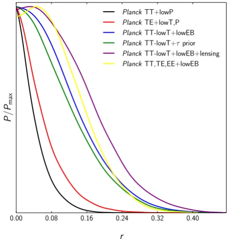
r0.002 < 0.10 (95% CL,PlanckTT+lowP), (22) r0.002 < 0.11 (95% CL,PlanckTT+lowP+lensing), (23) r0.002 < 0.11 (95% CL,PlanckTT+lowP+BAO), (24) r0.002 < 0.10 (95% CL,PlanckTT, TE, EE+lowP). (25)
Table4also shows the bounds onnsin each of these cases.
These results slightly improve over the constraint r0.002 <
0.12 (95% CL) derived from thePlanck2013 temperature data in combination with WMAP large-scale polarization data (Planck Collaboration XVI 2014;Planck Collaboration XXII 2014). The constraint obtained byPlanck temperature and polarization on large scales is tighter than thePlanck B-mode 95% CL upper limit from the 100 and 143 GHz HFI channels,r<0.27 (Planck Collaboration XI 2016). The constraints onrreported in Table4 can be translated into upper bounds on the energy scale of in-flation at the time when the pivot scale exits the Hubble radius using
V∗=
3π2A s
2 r M
4
pl=(1.88×10
16GeV)4 r
0.10· (26)
This gives an upper bound on the Hubble parameter during in-flation ofH∗/Mpl<3.6×10−5(95% CL) forPlanckTT+lowP.
These bounds are relaxed when allowing for a scale depen-dence of the scalar and tensor spectral indices. In that case, we assume that the tensor spectral index and its running are fixed by the standard inflationary consistency condition at second order in slow roll. We obtain
r0.002< 0.18 (95% CL,PlanckTT+lowP), (27)
dns
dlnk = −0.013
+0.010
−0.009 (68% CL,PlanckTT+lowP), (28)
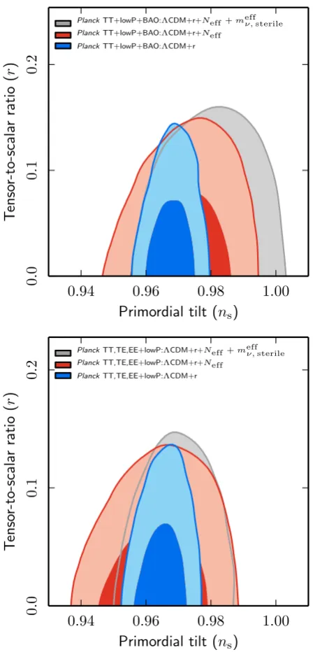
withns=0.9667±0.0066 (68% CL). At the standard pivot scale, k∗ = 0.05 Mpc−1, the bound is stronger (r <0.17 at 95% CL),
becausek∗ is closer to the scale at whichns andr decorrelate.
The constraint onr0.002in Eq. (27) is 21% tighter than the
corre-spondingPlanck2013 constraint. The mean value of the running in Eq. (28) is higher (lower in absolute value) than withPlanck
0.92 0.94 0.96 0.98 1.00
ns
−
0
.
04
0
.
00
0
.
04
Running
sp
ectral
index
dn
s
/d
ln
k
Planck 2013 Planck TT+lowP Planck TT,TE,EE+lowP
Fig. 5.Marginalized joint confidence contours for (ns,dns/dlnk), at the
68% and 95% CL, in the presence of a non-zero tensor contribution, and usingPlanckTT+lowP orPlanckTT, TE, EE+lowP. Constraints from thePlanck2013 data release are also shown for comparison. The thin black stripe shows the prediction of single-field monomial inflation models with 50<N∗<60.
0.94 0.96 0.98 1.00
Primordial tilt (ns)
0
.
00
0
.
15
0
.
30
T
ens
or
to
scal
ar
ra
tio
r
Planck2013 PlanckTT+lowP PlanckTT,TE,EE+lowP
Fig. 6.Marginalized joint confidence contours for (ns,r), at the 68%
and 95% CL, in the presence of running of the spectral indices, and for the same data combinations as in the previous figure.
the lensing reconstruction, BAO, or high-`polarization data. The tightest bounds are obtained in combination with polarization:
r0.002<0.15
(95% CL,PlanckTT, TE, EE+lowP), (29) dns
dlnk=−0.009±0.008
(68% CL,PlanckTT, TE, EE+lowP), (30) withns=0.9644±0.0049 (68% CL).
Neither thePlanckfull mission constraints in Eqs. (22)−(25) nor those including a running in Eqs. (27) and (29) are com-patible with the interpretation of the BICEP2B-mode polariza-tion data in terms of primordial gravitapolariza-tional waves (BICEP2 Collaboration 2014b). Instead they are in excellent agree-ment with the results of the BICEP2/Keck Array-Planck cross-correlation analysis, as discussed in Sect.13.
5.2. Dependence of therconstraints on the low-`likelihood
The constraints on r discussed above are further tightened by adding WMAP polarization information on large angular scales. ThePlanckmeasurement of CMB polarization on large angular scales at 70 GHz is consistent with the WMAP 9-year one, based on theK,Q, andV-bands (at 30, 40, and 60 GHz, respectively), once the Planck 353 GHz channel is used to remove the dust contamination, instead of the theoretical dust model used by the WMAP team (Page et al. 2007). (For a detailed discussion, see Planck Collaboration XI 2016.) By combiningPlanck TT data with LFI 70 GHz and WMAP polarization data on large angular scales, we obtain a 35% reduction of uncertainty, giving τ = 0.074±0.012 (68% CL) and ns = 0.9660±0.060 (68% CL)
for the baseΛCDM model. When tensors are added, the bounds become
r0.002<0.09 (95% CL,PlanckTT+lowP+WP), (31) ns=0.9655±0.058 (68% CL,PlanckTT+lowP+WP), (32) τ=0.073−+00..011013 (68% CL,PlanckTT+lowP+WP). (33) When tensors and running are both varied, we obtain r0.002 <
0.14 (95% CL) and dns/dlnk = −0.010 ±0.008 (68% CL)
forPlanckTT+lowP+WP. These constraints are all tighter than those based onPlanckTT+lowP only.
5.3. The tensor-to-scalar ratio and the low-`deficit in temperature
As noted previously (Planck Collaboration XV 2014; Planck Collaboration XVI 2014;Planck Collaboration XXII 2014), the low-`temperature data display a slight lack of power compared to the expectation of the best-fit tensor-free baseΛCDM model. Since tensor fluctuations add power on small scales, the effect will be exacerbated in models allowingr>0.
In order to quantify this tension, we compare the observed constraint onrto that inferred from simulated Planckdata. In the simulations, we assume the underlying fiducial model to be tensor-free, with parameters close to the baseΛCDM best-fit val-ues. We limit the simulations to mock temperature power spec-tra only and fit these specspec-tra with an exact low-`likelihood for 2≤`≤29 (seePerotto et al. 2006), and a high-`Gaussian like-lihood for 30 ≤ ` ≤ 2508 based on the frequency-combined, foreground-marginalized, unbinned Planck temperature power spectrum covariance matrix. Additionally, we impose a Gaussian prior ofτ=0.07±0.02.
Based on 100 simulated data sets, we find a 95% CL upper limit on the tensor-to-scalar ratio of ¯r2σ ≈ 0.260. The
corre-sponding constraint from real data (using low-` Commander
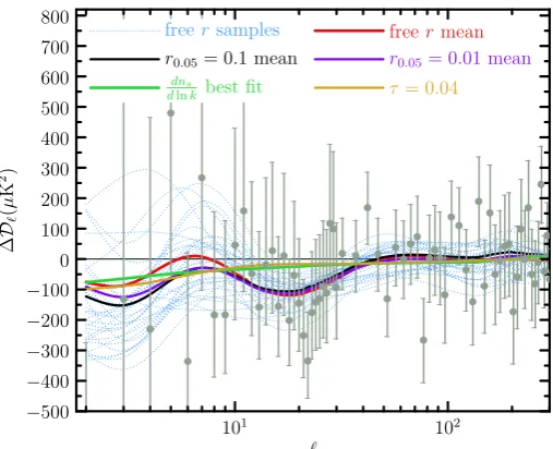
temperature data, the frequency-combined, foreground-marginalized, unbinned Planck high-` TT power spectrum, and the same prior onτas above) readsr <0.123, confirming that the actual constraint is tighter than what one would have expected. However, the actual constraint is not excessively unusual: out of the 100 simulations, 4 lead to an even tighter bound, corresponding to a significance of about 2σ. Thus, under the hypothesis of the base ΛCDM cosmology, the upper limit onr that we get from the data is not implausible as a chance fluctuation of the low multipole power.
To illustrate the contribution of the low-`temperature power deficit to the estimates of cosmological parameters, we show as an example in Fig.7howns shifts towards lower values when