Analytical Bounding Data Cache Behavior for Real-Time Systems

(1)

RAMAPRASAD, HARINI Analytically Bounding Data Cache Behavior for Real-Time Sys-tems. (Under the direction of Associate Professor Frank Mueller).

This dissertation presents data cache analysis techniques that make it feasible to

predict data cache behavior and to bound the worst-case execution time for a large class of

real-time programs.

Data Caches are an increasingly important architectural feature in most modern

computer systems. They help bridge the gap between processor speeds and memory access

times. One inherent diﬃculty of using data caches in areal-time systemis the unpredictabil-ity of memory accesses, which makes it diﬃcult to calculate worst-case execution times of

real-time tasks.

This dissertation presents an analytical framework that characterizes data cache

behavior in the context of independent, periodic tasks with deadlines less than or equal to

their periods, executing on a single, in-order processor. The framework presented has three

major components.

1) The ﬁrst component analytically derivesdata cache reference patternsfor all scalar and non-scalar references in a task. Using these, it produces a safe and tight upper

bound on the worst-case execution time of the task without considering interference from

other tasks.

2) The second component calculates the worst-case execution time and response

time of a task in the context of a multi-task, prioritized, preemptive environment. This

component calculatesData-Cache Related Preemption Delayfor tasks assuming that all tasks in the system are completely preemptive.

3) In the third component, tasks are allowed to havecritical sections in which they access shared resources. In this context, two analysis techniques are presented. In the

ﬁrst one, a task executing in a critical section is not allowed to be preempted by any other

task. In the second one, the framework incorporates Resource Sharing Policies to arbitrate

accesses to shared resources, thereby improving responsiveness of high-priority tasks that

do not use a particular resource.

In all the components presented in this dissertation, a direct-mapped data cache

is assumed. Experimental results demonstrate the value of all the analysis techniques

(2)

by

Harini Ramaprasad

A dissertation submitted to the Graduate Faculty of North Carolina State University

in partial fullfillment of the requirements for the Degree of

Doctor of Philosophy

Computer Science

Raleigh, North Carolina

2008

APPROVED BY:

Dr. Tao Xie Dr. Eric Rotenberg

Dr. Frank Mueller Dr. Vincent Freeh

(3)

BIOGRAPHY

Harini Ramaprasad was born on 6th November 1979, in Bangalore, India. She received her Bachelor of Engineering degree in Computer Science from Bangalore University, India

in September 2001. In fall of 2002, she came to the North Carolina State University to

pursue graduate studies in Computer Science. She received her Master of Science degree

in Computer Science from North Carolina State University in May 2006. She will receive

the Doctor of Philosophy degree in Computer Science from North Carolina State University

(4)

ACKNOWLEDGMENTS

This dissertation would not have been possible without guidance from my PhD advisor, Dr.

Frank Mueller. I would like to thank him immensely for his support and patience. I would

like to thank Dr. Vincent Freeh, Dr. Tao Xie and Dr. Eric Rotenberg for being on my

advisory committee. I would like to thank my colleague, Sibin Mohan, for his support in the

development of the static timing analyzer used in this dissertation. I would like to express

my immense gratitude towards my friends Yatin Tawde and Meghana Velegar for all their

support. Lastly, I would like to thank my husband, Gopalakrishnan Santhanaraman, and

(5)

LIST OF TABLES

Table 4.1 Characteristics of Variables . . . 24

Table 4.2 Coyote Output vs. Data Cache Analyzer Output (Hit: dot, Miss: M) . . . 25

Table 4.3 Comparison: Coyote/Data Cache Analyzer/Trace-Driven for 4KB Data Cache . . . 29

Table 4.4 Per-Reference Misses by Data Cache Analyzer vs. Trace-Driven for matrix1 30 Table 4.5 Timing Analysis for Diﬀerent Data Cache Categorizations in Cycles. . . 31

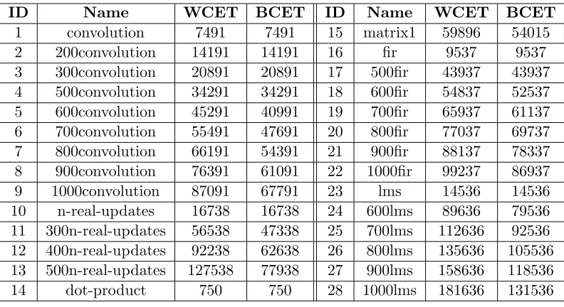
Table 5.1 Stand-Alone WCETs and BCETs of DSPStone Benchmarks . . . 34

Table 6.1 Example Task Set Characteristics - Task Set 1 . . . 39

Table 6.2 Task Set, Optional Phasing . . . 41

Table 6.3 Example Task Set Characteristics - Task Set 2 . . . 43

Table 6.4 Task Set Characteristics: Benchmark IDs and Periods [cycles] for Task Sets 59 Table 6.5 Analysis Times in Seconds . . . 63

Table 6.6 Number of Preemptions (# P) for Task Set with U = 0.5 . . . 65

Table 6.7 Number of Preemptions (# P) for Task Set with U = 0.8 . . . 65

Table 6.8 # Preemptions for Task Sets with U=0.5 and U=0.8 . . . 68

Table 7.1 Task Set Characteristics - Task Set 1 [RM policy→T₀has Highest Priority] 75 Table 7.2 Example Task Set Characteristics - Task Set 2 . . . 79

Table 7.3 Characteristics of Regions of Tasks with NPR . . . 91

Table 7.4 Task Set Characteristics: Benchmark IDs, Phases[cycles] and Periods [cycles] 92 Table 7.5 WCET/BCET Ratios forT₂. . . 96

(9)

Table 8.2 Task Set Characteristics - Task Set 2 [T₀ has Highest Priority] . . . 102

Table 8.3 Task Set Characteristics for Resource Sharing Tasks . . . 115

Table 8.4 Resource Usage Characteristics . . . 116

(10)

LIST OF FIGURES

Figure 2.1 Hard versus Soft Real-Time Systems . . . 5

Figure 2.2 Static Timing Analysis Framework . . . 8

Figure 2.3 Memory Hierarchy in a Typical Computer System . . . 9

Figure 2.4 Possible Mappings Between Main and Cache Memories . . . 11

Figure 4.1 Loop Nest and Iteration Space with one Reuse Vector r = (0,0,1) for A[k][i] . . . 16

Figure 4.2 Data Cache Analyzer: Enhanced Coyote Framework . . . 20

Figure 4.3 Forced Loop Fusion Pseudocode . . . 21

Figure 4.4 Example Illustrating Forced Loop Fusion . . . 22

Figure 4.5 Sample Mapping of 2-D Column-Major Array in Cache . . . 23

Figure 4.6 Loop Transformation . . . 25

Figure 4.7 Static Timing Analysis Framework Enhanced with Data Cache Analyzer . 26 Figure 4.8 Miss Pattern Crossing Loop Nests . . . 28

Figure 6.1 Access Chains for Cache Lines 1, 2 and 3 . . . 37

Figure 6.2 Distribution of Preemption Costs Across the Iteration Space . . . 40

Figure 6.3 Preemption with Synchronous Release . . . 42

Figure 6.4 Preemption with Φ Phasing . . . 42

Figure 6.5 Timeline for TaskT₁. . . 44

Figure 6.6 Timeline for TaskT₂. . . 44

Figure 6.7 Creation Dependencies among Event Types . . . 50

(11)

Figure 6.9 Algorithm (cont.) for Calculation of WCET w/ Delay . . . 52

Figure 6.10 Algorithm (cont.) for Calculation of WCET w/ Delay . . . 53

Figure 6.11 Results for U=0.5 using RM Policy . . . 61

Figure 6.12 Results for U=0.8 using RM Policy . . . 62

Figure 6.13 Results for U = 0.5 (Staggered - Synchronous) . . . 66

Figure 6.14 Results for U = 0.8 (Staggered - Synchronous) . . . 67

Figure 6.15 # Preemptions given by OurFP-RangeMax for Varying WCET/BCET . . 69

Figure 6.16 Comparison of Results for RM and EDF for U=0.5 . . . 71

Figure 6.17 Comparison of Results for RM and EDF for U=0.8 . . . 72

Figure 7.1 Best and Worst Case Results for Task Set 1 . . . 76

Figure 7.2 Best and Worst-Case Scenarios for Task Set 2 . . . 80

Figure 7.3 Algorithm for NPR-Aware Calculation of WCET w/ Delay . . . 83

Figure 7.4 Algorithm (cont.) for NPR-Aware Calculation of WCET w/ Delay. . . 84

Figure 7.7 Results for U=0.5 under RM and EDF Scheduling . . . 93

Figure 7.8 Results for U=0.8 under RM and EDF Scheduling . . . 94

Figure 7.9 Response Times of Tasks . . . 96

Figure 8.3 Algorithm to Calculate D-CRBD . . . 105

(12)

Figure 8.6 Algorithm (cont.) for Calculation of WCET w/ Delay for Resource-Sharing

Tasks . . . 108

Figure 8.7 Algorithm (cont.) for Calculation of WCET w/ Delay for Resource-Sharing Tasks . . . 109

Figure 8.8 Results for U=0.5 using RM and EDF Policies . . . 117

Figure 8.9 Results for U=0.8 using RM and EDF Policies . . . 118

Figure 9.1 Preemption with Φ Phasing . . . 124

(13)

Chapter 1

Introduction

In this chapter, the basic motivation for the work presented in this dissertation is

provided, followed by a brief outline of its primary contributions.

1.1

Motivation

In recent times, embedded systems have become ubiquitous. They have numerous

applications ranging from cell-phones and hand-held devices to aircraft control systems

and space explorers. Several embedded systems have hard real-time requirements, which,

in addition to logical constraints, introduce temporal constraints on the tasks (programs)

executing on such systems . These temporal constraints are in the form of a deadline by which a task must complete its execution.

The process of determining whether a given set of tasks can be scheduled on a

real-time system such that no task violates its temporal constraints is known as schedulability

analysis. This analysis requires a-priori knowledge of the execution time of every task in the system.

The execution time of a task is not a constant and its calculation is not

straight-forward due to several reasons. First of all, programs do not follow the same execution

path every time they are executed due to diﬀerences in input data. Furthermore, the

ex-ecution time of a given exex-ecution path varies between exex-ecutions due to eﬀects of several

architectural features of the system and due to the presence of other tasks in the system.

In order to guarantee adherence to the temporal constraints imposed on a

(14)

bound is termed Worst-Case Execution Time (WCET) of the task. While calculating the

WCET of a task, the eﬀects of all architectural features and of other tasks in the system

must be taken into account. In a situation where the eﬀects are ambiguous, the worst-case

behavior must be assumed in order to maintain safety of the system.

Caches are an invaluable architectural feature in today’s higher-end processors.

The savings they provide in terms of memory latency are immense. Hence, they have become

indispensable. Nonetheless, caching has one inherent complexity, namely, the latency of a

memory access becomes unpredictable.

An instruction cache may be analyzed to determine the latency of accessing an

instruction depending on whether it is found in the instruction cache or not. However, data

caches are much more diﬃcult to analyze since a single memory access instruction (reference)

could access diﬀerent memory locations at diﬀerent points in time. The simplest example

of such a case is an access to an array element within a loop. In every iteration of the loop,

a diﬀerent element in the array and, hence, a diﬀerent memory location, could be accessed.

Thus, data cache analysis for the purpose of static timing analysis, while challenging, is an

important problem.

While calculating the execution time of a single task is a necessary step in static

analysis, it is far from being suﬃcient in the presence of multiple tasks executing in a

prioritized manner. In this context, data caches introduce further complexity to static

analysis.

Hypothesis: Data cache behavior of a large class of programs executing in a multi-tasking, prioritized environment can be predicted using advanced static analysis

tech-niques.

1.2

Contributions of this Dissertation

This dissertation proposes analysis techniques to characterize data cache behavior

in the context of hard real-time systems. The contributions of this dissertation may be

categorized as follows.

1. Single task analysis: Here, an analysis technique that derives a safe and tight upper

bound on the worst-case execution time of a single task using data cache reference

(15)

2. Preemptive tasks: Here, analysis techniques are presented to calculate safe and tight

upper bounds on the response times of multiple tasks executing in a prioritized,

fully-preemptive manner.

3. Tasks with critical sections: Here, analysis techniques that produce safe and tight

upper bounds on the response times of tasks that may contain critical sections are

presented.

The rest of this dissertation is organized as follows. Chapter 2 provides required

background information and Chapter 3 presents the task model used in this dissertation.

Chapter 4 presents techniques to analyze a single task. Chapter 5 introduces a multi-task

execution environment. Chapters 6, 7 and 8 present analysis techniques for multiple tasks

executing in a prioritized manner for fully-preemptive tasks, tasks with a non-preemptive

region and tasks that execute in accordance with resource-sharing protocols, respectively.

Chapter 9 discussed related work and Chapter 10 summarizes the contributions of this

(16)

Chapter 2

Background Information

This chapter provides background information required for the topic of this

disser-tation. Section 2.1 describes the basics of real-time systems and Section 2.2 introduces the

concept of timing analysis in real-time systems. Section 2.3 describes memory hierarchies

in most modern computer systems, with particular focus on cache memories.

2.1

Real Time Systems

A real-time computer system is one in which, in addition to logical constraints,

tasks have temporal constraints to meet. In other words, for every task executing in a

real-time environment, there is a speciﬁc deadline — a time before which the task must complete its execution [1].

2.1.1 Hard and Soft Real-Time Systems

There are two types of real-time systems, namely hard and soft real-time systems.

In hard real-time systems, the temporal constraints that are placed on tasks are rigid

[2]. If a task does not adhere to these and exceeds its deadline, the consequences are

usually severe. Examples of a hard real-time system include aircraft control systems, space

explorers, emergency life-support systems, etc. In such systems, completion of an operation

after its deadline is considered useless and may lead to failure of the system.

On the other hand, in soft real-time systems, the temporal constraints are more

relaxed. In such a system, the usefulness of results obtained from a task does not drop to zero

(17)

quality of service is maintained, a task may miss a few deadlines. An example of a soft

real-time system is a multimedia streaming application. Figure 2.1 depicts the usefulness

of results with respect to the deadline of a task in hard and soft real-time systems.

Time

Hard Real−Time Soft Real−Time 100%

Usefulness

_Deadline

Figure 2.1: Hard versus Soft Real-Time Systems

2.1.2 Real-Time Tasks

There are two types of real-time tasks, namely, periodic tasks and aperiodic

(spo-radic) tasks. In the case of a periodic task, an instance, termed as a job, of the task is released at ﬁxed intervals of time. Therelease point of a task represents the time at which it isreadyfor execution. On the other hand, an aperiodic task is one which has aminimum inter-arrival time between its instances, but not a ﬁxed one. In this dissertation, the focus

is on periodic, hard real-time systems.

Every periodic task possesses the following characteristics.

1. Phase: This represents the time between the start of the system and the release of

the ﬁrst instance of a task.

2. Period: This represents the inter-arrival time between two consecutive instances of a

task.

3. Worst-Case Execution Time: This represents a guaranteed upper bound on the

(18)

4. Relative Deadline: This represents the time by which every instance of a task must

complete its execution, relative to its own time of release.

2.1.3 Schedulability Analysis

Schedulability analysis of a real-time system refers to the process of checking the

feasibility of execution of a given set of tasks such that no task instance misses its deadline.

In order to perform this analysis, the four basic characteristics of every task must be known

a-priori[3].

2.2

Timing Analysis

Timing analysis refers to the process of determining the execution time of a given

program. In the context of real-time systems, timing analysis is used to calculate the

worst-case execution time of a task, a characteristic that must be known a-priori for conducting schedulability tests on a set of real-time tasks. There are two fundamental approaches to

timing analysis, namely, dynamic timing analysis and static timing analysis.

2.2.1 Dynamic Timing Analysis

Dynamic timing analysis methods, also known as measurement-based timing

meth-ods, estimate the execution time of a given task either by actually executing the task or by

simulating the execution of the task repeatedly using diﬀerent sets of input data.

It has been demonstrated in earlier studies that dynamic analysis by actual

execu-tion of a task does not guarantee worst-case estimates [4]. Furthermore, exhaustive testing

of the input space is impractical. In the context of a real-time system, specially in the case

of a hard real-time system, temporal guarantees are vital to the safety of the system, hence

making dynamic timing analysis unsuitable in general.

2.2.2 Static Timing Analysis

Static timing analysis is the process of determining the worst-case execution time

of a task without actually executing or simulating the execution of the task. Analytical

models of all the components of a system (both hardware/architectural components and

(19)

traversed and, using the models, the eﬀects of all possible inputs on the control ﬂow of a

program are determined.

The result of such an analysis is a possibly conservative, yet safe upper bound on the execution time of the task. Due to this feature, static timing analysis is a method

for determining the worst-case execution time of tasks in the context of a hard real-time

system that raises the conﬁdence in the temporal correctness of a system. In the rest of

this dissertation, the focus is on static timing analysis.

2.2.3 Unpredictability in Static Timing Analysis

Static timing analysis typically consists of three diﬀerent phases.

1. Low-level analysis: In this phase, execution times are calculated for all atomic

in-structions in the instruction set for the architecture under consideration.

2. Flow analysis: In this phase, the control-ﬂow graph of the task being analyzed is

traversed to construct paths of execution.

3. WCET calculation: In this phase, analytical models of the components of the system

are used in conjunction with information gleaned from the low-level and ﬂow analyses

to determine the worst-case execution time of a task.

While the ﬁrst two phases are fairly straightforward, the structure and control

ﬂow of a program may cause signiﬁcant hurdles in the last phase of static timing analysis.

Factors such as data-dependent control ﬂow, indirect memory accesses via pointers, dynamic

memory accesses, etc. may cause unpredictability in the process.

Furthermore, the correctness of static timing analysis relies on the correctness

and precision of the analytical models of architectural components of the system. Several

modern architectural features such as caches, pipelines, branch predictors, etc. are hard

to model. One feature that is particularly hard to model is the data cache. While data caches are very useful to improve the average-case performance of a system, its worst-case

behavior is not easily predictable. Hence, data cache analysis has hence been the focus of

much research in recent years.

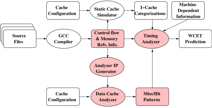
The static timing analyzer framework used in this dissertation is shown in Figure

2.2 [5, 6, 7, 8]. Source ﬁles constituting a program are ﬁrst compiled using an enhanced

(20)

Files

Cache Configuration

Control flow & Memory

Refs. Info. Analyzer GCC

Compiler Prediction

WCET Source

I−Cache Categorizations Static Cache

Simulator

Machine

Information Dependent

Timing

Figure 2.2: Static Timing Analysis Framework

program. This information is fed to a static cache simulator that simulates theinstruction cache to produce instuction cache categorizations for the given program. The instruction cache categorizations, along with some machine-dependent information, are fed to the core

timing analyzer that then calculates an upper bound for the worst-case exeution time of a

task.

It may be observed that there is no data cache analysis incorporated in this

frame-work. In Chapter 4, this issue is addressed, and a framework for data cache analysis is

presented. The data cache analysis framework is then integrated into the static timing

analyzer shown in Figure 2.2.

2.3

Cache Memory

While the processing power and speed of a processor double almost every 18

months, the same cannot be said about the speed of the memory that they need to access

frequently. In order to bridge this gap between the processor speeds and memory speeds,

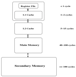
most modern processors have a memory hierarchy in place. A typical memory hierarchy is

shown in Figure 2.3. A register ﬁle, located in the processor core itself, is the fastest and

smallest memory in the hierarchy. Disk memory is the slowest and largest memory and is

located far away from the processor. Since faster technology is more expensive, the size of

the memory is forced to be smaller as the memory gets faster. Hence, the amount of storage

decreases moving from lower levels of memory to upper levels [9, 10, 11, 12].

The basic principle that enables such a memory hierarchy to bridge the gap

be-tween processor speeds and memory access times is locality of reference. In simple terms, this principle refers to the fact that, if a certain memory element is accessed at a certain

(21)

L1 Cache

L2 Cache

>> 100 cycles

40−100 cycles

5−15 cycles

1−2 cycles

< 1 cycle

Main Memory

Secondary Memory Register File

Figure 2.3: Memory Hierarchy in a Typical Computer System

the same memory line will be accessed in the near future. The former is termed temporal locality and the latter,spatial locality.

A cache is a small, fast area of memory that is located on or close to the processor

chip. It stores frequently accessed memory lines for fast retrieval. When a program executes

a memory access instruction, the ﬁrst step is to check whether this requested memory line

is already in the cache. If the requested memory line is located in cache, acache hitoccurs. Otherwise, a cache missoccurs.

The number of cycles required to retrieve the requested data from lower levels

in the memory hierarchy is termed miss penalty. Cache misses are classiﬁed into three categories, namely, compulsary, capacity and conﬂict. Compulsary misses, also known as

cold misses, are the ones that are incurred the ﬁrst time a certain memory line is brought

into the cache. Capacity misses occur when the cache is not large enough to hold a program’s

entire working set. Conﬂict misses occur if two memory lines map to the same cache line.

(22)

2.3.1 Cache Organization

Every memory line in the main memory maps to a certain line in the cache memory.

Since the main memory is much larger than cache, this mapping is many-to-one. There are

three cache organizations based on the mapping function used.

1. Direct mapped: In a direct mapped cache, a certain memory line can map only to

one speciﬁc line in the cache. The cache line is determined by performing a modulo

operation on the address of the memory line.

2. Fully Associative: This is on the other end of the spectrum, where a certain memory

line can be mapped to any line in cache. Hence, the mapping is not dependent on

memory address, but rather on the usage of the cache.

3. Set associative (k-way): In this method, the cache is divided into sets. Each set consits

ofkcache lines. A modulo operation on the address of a memory line determines which

cache set is to be used. The memory line may then be placed in any cache line within

the identiﬁed set. A fully associative cache is a set associative cache with just one set

and a direct mapped cache, a 1-way set associative cache.

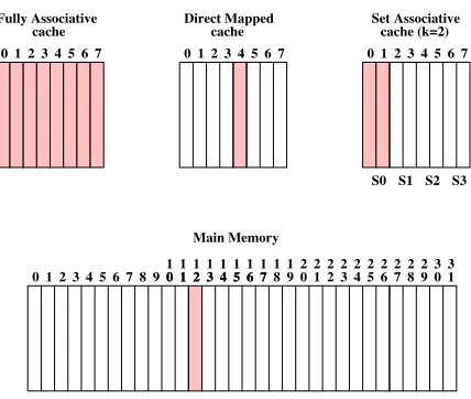
Figure 2.4 depicts these three diﬀerent cache organizations and shows which cache

lines a particular memory line may be mapped to. This memory line is represented by a

shaded rectangle, and the cache lines that it may be mapped to in the diﬀerent organizations

are also represented by shaded rectangles. The numbers above each rectangle representing

a memory line or a cache line are line numbers. In the case of set-associative caches, the

labels (preﬁxed by S) below indicate set numbers. In this example, the set associative cache

has an associativity of 2, indicating a set size of two.

2.3.2 Replacement Policy

Multiple memory lines that map to the same cache line could replace each other

in cache. In a direct mapped cache, this replacement is straightforward since every memory

line maps to one speciﬁc cache line. In case of a set associative cache, when a set is full,

any new memory line that maps to the same set has to replace one of the memory lines that already exist in the set. Now, there arises the question of which line to select for

replacement. There are several replacement policies and some of the commonly used ones

(23)

Set Associative

1 2 3 4 5 6 7 0 1 2 3 4 5 6 7 0 1 2 3 4 5 6 7

0 0 0

0

1 1 1

1

2 2 2

2

3 3 3

3

4 4 4

4

5 5 5

5

6 6 6

6

7 7 7

7 8 91 1 1 1 1 1 1 1 1 1 2 2 2 2 2 2 2 2 2 2 3 38 9 8 9 0 1 S1 S2 S3 S0

Main Memory Fully Associative

cache Direct Mappedcache cache (k=2)

0

Figure 2.4: Possible Mappings Between Main and Cache Memories

1. First In First Out (FIFO): Here, the line which was brought into the cache the earliest

is the ﬁrst to be replaced.

2. Least Recently Used (LRU): This policy replaces the cache line that was used the

longest time ago.

3. Random: As the name suggests, in this case, a cache line is chosen at random for

replacement.

2.3.3 Write Policy

Memory accesses may be of two types: read and write. When a memory write is

performed, there are two issues that need to be considered, namely, the issue of bringing

the accessed memory line into cache and the issue of writing the modiﬁed data into main

memory. There are four policies based on these issues.

1. Write Through: When a memory write is performed, the modiﬁed contents are written

through to the cache and the main memory.

2. Write Back: When a memory write is performed, it is written only to the cache. It is

written to main memory later when the cache line is replaced.

3. Write Allocate: The memory line is modiﬁed and then brought into the cache.

(24)

Systems specify a write policy for both a cache hit and a cache miss. The two

most commonly used combinations of policies are the write through with no write allocate

and the write back with write allocate.

2.3.4 Instruction and Data Caches

Instructions used to execute a program and data used by programs are both stored

in memory. Since the way that instructions are interpreted and used is diﬀerent from the

way that data is used, typically, at the higest level of cache, there is a segregation between

the part that holds instructions and the part that holds data. These are known as the

(25)

Chapter 3

Task Model

In the work presented in this dissertation, the focus is on periodic, hard

real-time tasks. Every task is assumed to have a deadline less than or equal to its period, an

assumption that is reasonable in a majority of hard real-time systems.

A task is assumed to have two types of characteristics, namelybasic and derived. A basic characteristic of a task is one that is defined for a specificsingletask, and a derived characteristic is one that is defined in the context of a given setof tasks.

As introduced in Section 2.1.2, every periodic real-time task has four basic

char-acteristics. In addition to these four characteristics, a task may have more characteristics,

both basic and dervied. The notations used in this dissertation for the basic and derived

characteristics of a task are now presented.

A task is denoted byTi, where iis a unique identiﬁer assigned to the task. The jth instance of Ti is denoted as job Ji,j. Thebasic characteristics of Ti are represented by the 5-tuple (Φi,Pi,Ci,ci,Di).

1. Φi represents the phase of a task, i.e., the time between the start of the system and the release of the ﬁrst instance of the task (ﬁrst job).

2. Pi represents the period of a task, i.e., the inter-arrival time between consecutive instances of the task.

3. Ci represents the worst-case execution time (WCET), of a task, i.e., the longest possible execution time for the task.

(26)

execution time for the task.

5. Di represents the relative deadline of a task, i.e., the time by when the task must complete its execution relative to its time of release.

In the context of a speciﬁc task set, a task has a set of derived characteristics,

represented by the 3 tuple (Bi,i, ∆i).

1. Bi represents theblocking time of a task, i.e., the time for which its execution might be interrupted due to a task with lower priority that holds a shared resource required

by the task.

2. irepresents theresponse timeof a task,i.e., the time between the release of the task and its completion.

3. ∆i represents thedata-cache related delay incurred by a task due to interruptions by other tasks.

The lowest common multiple (LCM) of the periods of all tasks within a task set

is known as thehyperperiod of the task set.

The work presented in this dissertation is divided into three major components. In

the ﬁrst component, data cache behavior is characterized with respect to a single task. In

this component, only four basic characteristics of a task are used — phase, period, WCET

and relative deadline. In the second component, the concept of preemptions among tasks

is introduced. In this component, one basic characteristic and three derived characteristics

are added to every task. The basic characteristic added is the best-case execution time of

the task. The derived characteristics, in the context of a task set, are response time and

data-cache related delay. In the ﬁnal component, a task may have critical sections within

its execution. In this context, every task has an additional derived characteristic, namely

(27)

Chapter 4

Data Cache Analysis - Single Task

In this chapter, an analytical technique for statically characterizing data cache

behavior in the context of a single real-time task is presented. An existing data cache

analysis framework, known as the Cache Miss Equations framework [13] was enhanced to

analyze a single task and calculate the number and positions of data cache misses that the

task incurs.

First, background information about the Cache Miss Equations framework is

pro-vided. Next, the enhancements incorporated by the work presented in this chapter are

discussed. Finally, experimental results are provided.

4.1

Cache Miss Equations Overview

The Cache Miss Equation (CME) framework proposed by Ghosh et al. [13] is a

method to generate a set of linear Diophantine equations to characterize the behavior of a

data cache in loop nest oriented code consisting of scalar and non-scalar (array) memory

references.

4.1.1 Terminology Iteration Space

(28)

be represented as the iteration pointi= (1,2,3). The set of all iteration points for a given

loop nest is known as its iteration space.

Reference and Access

A reference is a static memory read or write instruction in the program. A

par-ticular execution of a reference is termed as a memory access.

Reuse Vectors

In order to summarize data reuse among references in loop nest oriented code,

the CME framework uses the concept of reuse vectors as deﬁned by Wolf and Lam [14].

If a reference accesses the same memory line in two iterationsi₁ andi₂, wherei₂ > i₁,

r =i₂−i₁ is called a reuse vector. For example, consider the matrix multiplication code

shown in Figure 4.1(a).

for(i = 0; i < N; ++i) for(k = 0; k < N; ++k)

for(j = 0; j < N; ++j)

C[j][i] += A[k][i] * B[j][k]

(a) Matrix Multiplication Code

r

i

j k

(b) Iteration Space for Matrix Multiplication Code

Figure 4.1: Loop Nest and Iteration Space with one Reuse Vectorr= (0,0,1) for A[k][i]

Here, the referenceB(j, k) has a reuse, which is represented by the reuse vector

(0,1,0). Reuse vectors are classiﬁed into four types as described below.

1. Self-temporal reuse A self-temporal reuse occurs when a reference accesses the same memoryelementin diﬀerent iterations.

(29)

3. Group-temporal reuse A group-temporal reuse occurs when diﬀerent references access the same memory element.

4. Group-spatial reuse A group-spatial reuse occurs when diﬀerent references access the same memory line.

Consider the matrix multiplication code in Figure 4.1(a) again. The iteration

space for this code is shown in Figure 4.1(b). An example reuse vectorr= (0,1,0) is shown

in the iteration space.

Perfectly Nested and Rectangular Loops

A perfectly nested loop is one in which all memory references are found in the

inner most loop of the loop nest. A rectangular loop is one in which the upper bound of an

inner loop does not depend on the current iteration of an outer loop.

4.1.2 Cache Miss Equations

CMEs are a set of equations whose solutions represent potential cache misses for references in a loop nest. They relate the iteration space of the loop nest, base addresses of

arrays, array sizes and the cache parameters in a precise fashion. For every reference, and

along every reuse vector for that reference, two kinds of CMEs are generated —cold miss equations and replacement miss equations. The term along a reuse vector means that, for a reference, only that reuse vector is assumed to be present, ignoring the presence of any

other reuse vectors.

Cold Miss Equations

Solutions to cold miss equations represent potential cold data cache misses. These

are misses that occur upon the ﬁrst access to a memory line, hence making themcompulsary by deﬁnition. Cold misses may occur in two cases, namely, when a reference reuses data

(30)

Replacement Miss Equations

Solutions to replacement equations account for the remaining misses, namely,

ca-pacity and conﬂict misses. For a given reference, replacement miss equations along a

par-ticular reuse vector represent interference with any other reference, including itself

(self-conﬂict).

Solving CMEs directly is computationally complex. However, mathematical

tech-niques for manipulating these equations are employed to make the process tractable [15, 16].

Solutions to each CME only representpotential cache misses. The eﬀects of multiple CMEs are composed to ﬁnd the actual miss points. A detailed description of the generation of CMEs and the algorithm to compute the actual misses may be found in [13].

4.1.3 CME Implementation Overview

In the work presented in this dissertation, an existing implementation of the CME

framework is re-used and enhanced. The original implementation framework, named Coy-ote, is derived from work by Bermudo et al. [15]. The Coyote framework utilizes basic reuse vectors as suggested in [14]. The Coyote framework is extended, in the work presented in

this dissertation, to take into account the precise shape of the iteration space. This

ex-tended Coyote framewok forms the data cache analyzer in Figure 4.7 of Section 2.2.2 and will be referred to as such in the remainder of this dissertation.

4.2

Conceptual Enhancements to the CME framework

The original CME framework imposes several restrictions on programs that it

can analyze. Fundamental among these are as follows. First, the upper bounds of all

loops must be known at compile-time. Second, array subscript expressions must be aﬃne

functions of the loop induction variables. Third, the program can contain only perfectly

nested, rectangular loops. Fourth, the program cannot contain data-dependent conditionals.

Several enhancements were introduced into the CME framework in order to relax some of

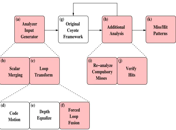
the above restrictions. These enhancements are depicted by the block diagram shown in

Figure 4.2.

Recent work by Vera et al. [17] relaxes the assumption about perfectly nested

(31)

This part of the loop transformation is done in the blocks (d) and (e) of Figure 4.2. A

disadvantage of this scheme is that it leads to changes in representation of reuse and iteration

spaces. In order to overcome this disadvantage and yet allow arbitrary loop nests, the

concept of forced loop fusion is introduced. This is represented by block (f) in Figure 4.2. These loop transformations are explained in detail in Section 4.3.

The enhanced framework permits non-rectangular loops in programs.

Conceptu-ally, a non-rectangular loop is represented by a condition posed on the upper bound of an

inner loop, based on the current value of the induction variable of an outer loop. They are

treated as such since any condition that is based solely on induction variables is analyzable

statically.

Finally, programs with data-dependent conditionals that have no “else” part are permitted. If the condition is not satisﬁed, one part of the code is simply skipped. An

upper bound on the number of misses incurred by a program with such a conditional is

calculated. For a direct-mapped cache, the worst case is to assume that the condition is

satisﬁed.

Since the data cache analyzer reuses the original Coyote framework (shown in block

(g) of Figure 4.2), up to the CME generation stage, the equations are generated assuming

that all references in the loop nest are executed at every point in the iteration space.

However, several statically analyzable conditionals are introduced during forced loop fusion

and while handling non-rectangular loop nests. Consequently, the reuse vectors generated

are no longer correct and could lead to overly optimistic (unsafe) or overly pessimistic

(unreal) results. To prevent timing violations and ensure timing safety, an extra analysis

step is added to the actual miss calculation stage. This step is represented by block (h) of

Figure 4.2.

4.3

Loop Transformations

The data cache analyzer performs several loop transformations on a program in

order to make programs with arbitrary loop nests analyzable by the CME framework. In

the ﬁrst step, the depths of all loop nests in the program are equalized by introducing

dummy loops with a single iteration where required. In the second step, forced loop fusion

is applied to these sequential loop nests of equal depth. The concept of forced loop fusion

(32)

Loop Transform (c) Scalar Merging (b) Misses Compulsory

Re−analyze (i) Hits Verify (j) Additional Analysis (h) (a) Analyzer Input Generator Framework Original Coyote (g) Miss/Hit Patterns (k) Forced Fusion Loop (f) Depth Equalize (e) Motion Code (d)

Figure 4.2: Data Cache Analyzer: Enhanced Coyote Framework

4.3.1 Forced Loop Fusion

Forced loop fusion is a technique whereby iteration spaces of several loop nests

of equal depth are concatenated to form one single loop nest. The basic idea behind this

technique is to concatenate iterations of all loops at the same depth. In order to maintain

the correct order of memory accesses within loops, conditionals based on the loop induction

variables are introduced as required.

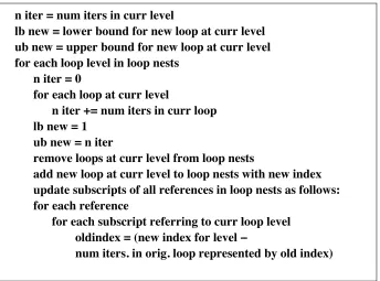
The algorithm for performing forced loop fusion is described in Figure 4.3. Fusion

starts from the outermost level and proceeds inwards. For every distinct level in the input

loop nests, a corresponding level is introduced in the fused output loop nest. The number

of iterations of the fused loop is the sum of the number of iterations of every loop at that

level in the input loop nests.

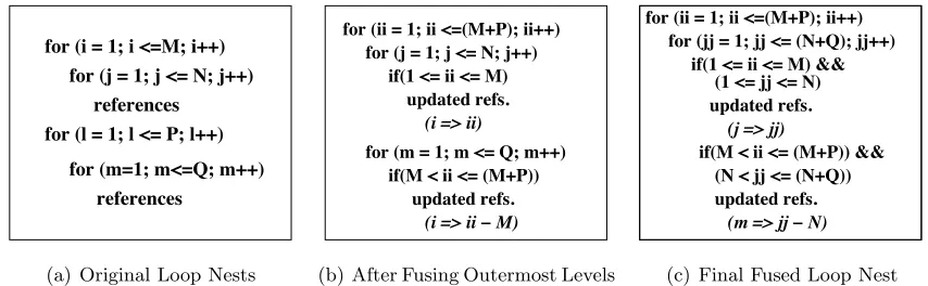
As an example, consider the loop nests shown in Figure 4.4(a). Here, the input

program has two distinct loop levels. Fusion is started at the outer loop level. Since there

are two loops at that level, with M and P number of iterations respectively, the outer

level of the fused loop nest would have a number of iterations equal to M +P. In order

to maintain the correct order of memory accesses, one conditional is introduced for each

reference in the innermost loop to specify when that reference is to be executed with respect

(33)

oldindex = (new index for level −

lb new = lower bound for new loop at curr level ub new = upper bound for new loop at curr level for each loop level in loop nests

n iter = 0

for each loop at curr level

n iter += num iters in curr loop lb new = 1

ub new = n iter

remove loops at curr level from loop nests

add new loop at curr level to loop nests with new index update subscripts of all references in loop nests as follows: for each reference

for each subscript referring to curr loop level n iter = num iters in curr level

num iters. in orig. loop represented by old index)

Figure 4.3: Forced Loop Fusion Pseudocode

in Figure 4.4(b). The same process is repeated for the subsequent levels in the input loop

nests until one single, perfectly nested loop is formed. The ﬁnal fused output loop nest

obtained in this example in shown in Figure 4.4(c).

4.4

Deriving Exact Data Cache Reference Patterns

The original CME work provides slightly pessimistic results for certain programs.

In addition to the conceptual enhancements presented in Section 4.2, new approaches are

proposed to overcome this pessimism.

4.4.1 Causes for Pessimism in CME Framework

Each individual CME only represents iteration points that couldpotentiallysuﬀer a data cache miss. These iteration points are then analyzed considering the combined eﬀect

of all reuse vectors for the reference, thus categorzing the reference as a miss or a hit in

the data cache for that particular iteration point. The CME framework produces slightly

(34)

for (l = 1; l <= P; l++) references

for (j = 1; j <= N; j++)

for (m=1; m<=Q; m++) references

for (i = 1; i <=M; i++)

(a) Original Loop Nests

(i => ii − M)

for (j = 1; j <= N; j++) if(1 <= ii <= M) for (ii = 1; ii <=(M+P); ii++)

updated refs.

(i => ii)

for (m = 1; m <= Q; m++) if(M < ii <= (M+P))

updated refs.

(b) After Fusing Outermost Levels

for (ii = 1; ii <=(M+P); ii++) for (jj = 1; jj <= (N+Q); jj++) if(1 <= ii <= M) &&

updated refs. (1 <= jj <= N) updated refs.

if(M < ii <= (M+P)) && (N < jj <= (N+Q))

(j => jj)

(m => jj − N)

(c) Final Fused Loop Nest

Figure 4.4: Example Illustrating Forced Loop Fusion

There are several reasons for this.

First, the implementation of CMEs, as provided by Coyote, does not analyze all

iteration points due to the complexity involved. Instead, a representative sample of the

iteration space is considered for analysis and a conﬁdence value is given as a feedback. The second problem stems from the layout of array elements in cache lines. In

the original CME framework by Ghosh et al. [13], all arrays are assumed to bealigned in memory lines and, hence, cache lines. This assumption might not always be true — the ﬁrst

element of an array may have a non-zero oﬀset from the start of the cache line. The Coyote

framework relaxes this assumption and takesexact base addresses into consideration during its analysis [15, 16]. However, even Coyote does not take arbitrary reuses into account.

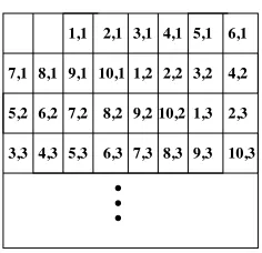
If arrays are not cache-aligned and elements are accessed in non-sequential order,

they may have reuses that the original CME framework does not detect. As an example,

consider a two-dimensional array a[1..10][1..10] that has a column-major layout. For the sake of simplicity, consider a data cache that is large enough to hold the array entirely. Let

the size of each cache line be 32 bytes and the size of each array element be 4 bytes. The

base address of the array is assumed to be such that it causes the the mapping shown in

Figure 4.5.

Now, consider an iteration space of depth two that traverses the array in

row-major order. The elements a[1][1], a[1][2] anda[1][3] are correctly categorized by the CME

framework as cold misses since it is the ﬁrst time those memory lines are accessed. Next,

elements like a[3][3] are also classiﬁed as cold misses since they are on a diﬀerent memory

line than previously accessed data. In a similar fashion, the CME framework also classiﬁes

(35)

6,2 7,2 1,3 2,3

4,3 5,3 6,3 8,3 9,3

1,1 4,1 5,1 6,1

7,1 8,1 9,1 2,2 3,2

8,2 9,2 10,2

3,3 7,3 10,3

2,1 3,1

10,1 1,2 4,2

5,2

Figure 4.5: Sample Mapping of 2-D Column-Major Array in Cache

asa[1][3], it has already been brought into the cache and should actually be classiﬁed as a

hit. Ignoring such reuse leads to pessimism in the miss count.

A third reason for pessimism in the CME framework is that it only captures reuse

between uniformly generated references. Reuse across variables is not captured. While

this impacts array references only for layouts where one array ends and another starts in

the same cache line, it severely impacts programs that have frequent references to scalar

variables that share cache lines due to their placement in memory.

4.4.2 Enhancements for Removal of Pessimism

In the work presented in this dissertation, the stress is on deriving exact data cache reference patterns. This makes it mandatory for the data cache analyzer to consider

all iteration points while computing actual miss points. This increases the complexity of computation. However, since the analysis is astatic one that pre-computes all data cache reference patterns by code analysis, thisone-time overhead is considered to be reasonable. Moreover, the improvement an exact pattern promises in accuracy of static timing analysis

for a single task is a signiﬁcant motivation for this approach in spite of the overhead.

The second problem described in Section 4.4.1 is not easy to resolve using reuse

vectors. Hence, a diﬀerent approach is taken and further analysis is performed on the

iteration points that are classiﬁed as compulsory misses by the CME framework. This is

represented by the block (i) in Figure 4.2. The analysis is as follows. First, a check is

conducted to see if there exists any prior iteration that references an element in the same

cache line as that of the reference under consideration. If so, a second check is conducted to

see if this reference has been replaced since it was last brought into the data cache. In order

(36)

used. Elements that map to the same cache line as the reference under consideration are

mapped back to the iteration space. This produces an iteration point that refers to these

elements. Afterwards, the check to ensure that this iteration point isearlier in the iteration space than the current iteration is a simple process. Since the number of elements that can

map to any cache line is a constant, the complexity involved in this process is generally

aﬀordable.

If a program has many scalars, the ﬁrst access to each of them is treated as a miss

by the original framework. Here, each variable would be considered separately and, hence,

reuse vectors do not capture reuse between them. In order to overcome this limitation,

scalars of equal size that are adjacent in memory aremerged and treated as an array for the purposes of data cache analysis. This merging is performed as part of a pre-analysis phase

as shown in block (b) of Figure 4.2. Hence, reuse between diﬀerent scalars that map to the

same cache line is captured by treating them as elements of a single array.

The result produced by the data cache analyzer, with the conceptual enhancements

presented in Section 4.2 and the enhancements presented in this section, is a series of data

cache miss/hit patterns - one for every reference in the program being analyzed.

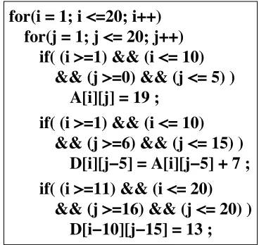
4.5

Putting it All Together: An Example

In this section, a simple example illustrating data cache analysis approach is

pro-vided. Consider a direct-mapped, 1 KB data cache with a line size of 32 bytes. The input

loop nests for the example task is shown in Figure 4.6(a). The input code consists of four

memory references, named 1, 2, 3 and 4 in the order of the ﬁrst execution of each reference.

Characteristics of the two variables in the code, namely, A and B, are shown in Table 4.1.

Table 4.1: Characteristics of Variables

Ref Dimensions Base Address Element Size

A 1..10, 1..10 151944 4

B 1..10, 1..10 153000 4

First, the input loop nests are pre-processed in accordance with the

transforma-tions described in Section 4.3.1. Recall that forced fusion concatenates loop bodies by

extending the ﬁrst iteration space with the second one. Loop bodies are conditionally

(37)

for(k = 1; k <= 10; k++)

for(j = 1; j <= 5; j++)

A[i][j] = 19 ;

for(i = 1; i <=10; i++)

D[s][m] = 13 ;

for(m = 1; m <= 5; m++)

for(s = 1; s <= 10; s++)

D[i][k] = A[i][k] + 7 ;

(a) Original Loop Nests

&& (j >=16) && (j <= 20) )

for(i = 1; i <=20; i++)

D[i

−

10][j

−

15] = 13 ;

for(j = 1; j <= 20; j++)

if( (i >=1) && (i <= 10)

&& (j >=0) && (j <= 5) )

A[i][j] = 19 ;

if( (i >=1) && (i <= 10)

&& (j >=6) && (j <= 15) )

D[i][j

−

5] = A[i][j

−

5] + 7 ;

if( (i >=11) && (i <= 20)

(b) Transformed Loop Nest

Figure 4.6: Loop Transformation

in Figure 4.6(b).

Using this transformed loop nest as input, cache miss equations are generated

using the data cache analyzer (extended Coyote framework). The miss/hit patterns that

are produced as a result are shown in Table 4.2. Column one shows the reference number.

Column two indicates the number of misses the original Coyote framework produces for the

given program and column three shows the results produced by the enhanced data cache

analyzer.

Table 4.2: Coyote Output vs. Data Cache Analyzer Output (Hit: dot, Miss: M)

Ref Coyote Data Cache Analyzer Output

misses Miss/Hit patterns

1 50 MMMMM...M... 2 100 ...MMMMM...M...M

...

3 100 MMMMMMMMMM...M...M...M ...

4 50 ...

The original Coyote framework cannot analyze loop nests with the structure shown

in Figure 4.6(a). It is given the transformed loop nest shown in Figure 4.6(b), but has no

(38)

framework assumes that all the references are executed at every point in the fused iteration

space and produces very pessimistic results.

On the other hand, the miss/hit patterns produced by the data cache analyzer are

accurate. They not only convey information about the number of misses for every reference,

but also about their positions in the access space of the reference.

4.6

Implications to the Static Timing Analyzer

The data cache analysis technique presented thus far in this chapter implies

sig-niﬁcant improvements to static timing analysis. The static timing analyzer framework

described in Section 2.2.2 is now enhanced to include the data cache analyzer. The

re-sulting framework is depicted in Figure 4.7. The shaded blocks represent the novel and

enhanced modules of the framework.

Control ﬂow and memory reference information is now fed to the input generator

module, which is responsible for performing scalar merging, loop transformations, etc. as

explained in Sections 4.3 and 4.4. The resulting single, perfectly nested loop is given to the

data cache analyzer, which then produces data cache miss/hit patterns, also termed data cache reference patterns. These patterns indicate which data cache accesses are guaranteed

Configuration

Miss/Hit I−Cache Categorizations Static Cache Simulator Machine Information Dependent Patterns WCET Prediction Timing Analyzer GCC Compiler Source Files Cache Configuration Analyzer IP Generator Data Cache Cache Control flow & Memory Refs. Info. Analyzer

(39)

to be hits and which others are not.

The data cache reference patterns indicate thepositionof each miss in a sequence of references. However, in this chapter, the aim is to obtain WCET estimates for a single task ignoring the interference from other tasks in the system. For this purpose, it is suﬃcient

to use just thenumber of data cache misses that a reference incurs. Hence, in this chapter, only the number of misses is fed to the core timing analyzer. The timing analyzer considers

the impact of these cache misses in the context of pipeline analysis and path traversal to

obtain bounds on the WCET of the task.

In order to obtainsafe and tight WCET bounds, static timing analysis considers one loop nest at a time starting with the inner-most nest. The times of the longest paths are

then repeatedly determined as long as a change in the cache or processor states is observed.

Asteady state is said to be reached when two consecutive loop iterations result in the same WCET bound. The remaining loop iterations are then guaranteed to be bound by this

ﬁxpoint as well [18]. The overall bound for an inner loop can be used directly in the context

of the outer loop in conjunction with adjustments due to caching eﬀects between loop

nests. This method assumes a consistent pattern for the worst-case cache categorization,

even across loops. While this assumption is valid in the case of an instruction cache, it may

not be valid for a data cache.

Considerndata cache misses for a reference, wherenmay exceed the upper bound

on the number of iterations for an inner loop. Hence, misses extend beyond the iterations of

the inner loop. Furthermore, these misses may be scattered over a subset of iterations of the

outer loop, not necessarily following any regular pattern, as was observed in the experiments.

To handle such misses, the next iteration of the outer loop needs to be considered when

ﬁnding a ﬁxpoint for the inner loop. This increases the number of iterations of the inner loop

that need to be considered before reaching a steady state, thus increasing the complexity of

static timing analysis. A method is now presented to solve this problem with a space and

time complexityO(r+ 1), wherer is the number of references in a loop nest.

To illustrate the solution, consider the code shown in Figure 4.8(a). For the sake

of demonstration, assume that the number of misses predicted by the data cache analyzer

for the refernceA[i][j] is 13. The innerjloop is timed once considering the referenceA[i][j]

(40)

for(i = 1; i < 10; ++i) for(j = 1; j <= 10; ++j

A[i][j] = 19;

(a) Sample Loop Nests

Iterations with Iterations with i miss time for j loop Hit time for j loop

1 10 0

2 3 7

3..10 0 10

(b) Miss and Hit Time

Figure 4.8: Miss Pattern Crossing Loop Nests

of the outer loop are propagated. Table 4.8(b) shows these values for the example being

considered.

This concept, when extended to a loop nest with several references, leads to an

al-gorithm with complexityO(r+ 1) since several permutations of miss/hit status of references

need to be considered unlike just two timings in the current example.

4.7

Experimental Setup

Several experiments are conducted to demonstrate the data cache analysis

tech-nique introduced in this chapter. In all experiments, a direct-mapped cache of size 1 kilobyte

is assumed unless otherwise mentioned. All but two of the benchmarks used in the

experi-ments are taken from the DSPStone benchmark suite [19].

These benchmark programs are modiﬁed to replace pointer-based memory accesses

with equivalent array accesses to make them statically analyzable. The concept of abstract inlining is used to inline all the functions in the benchmark due to implementation con-straints. Since these changes do not aﬀect the order of memory accesses in the benchmarks,

they are acceptable for the purposes of data cache analysis. Some of the benchmarks in

the DSPStone suite are not suitable since they have indirect memory accesses, which are

currently not analyzable by the data cache analyzer.

A sorting benchmark, simple-srt-test, is taken from the CLAB benchmark suite.

Lastly, a synthetic benchmark is contructed in order to assess the contributions of the data

(41)

Table 4.3: Comparison: Coyote/Data Cache Analyzer/Trace-Driven for 4KB Data Cache

Benchmark Coyote framework Data Cache Analyzer Simulator

used Misses Hits Misses Hits Misses Hits

convolution 400 400 26 374 26 374

dotproduct 8 0 3 5 1 7

ﬁr 599 1192 26 573 26 573

lms 1207 9449 27 1071 27 1071

matrix1 4600 779400 39 4561 38 4562

nrealupdates 1200 2400 52 1148 50 1150

simple-srt-test 14 59986 14 29686 14 29686

looptest 39 161 26 174 26 174

4.8

Experimental Results

In this section, results from experiments conducted using the benchmarks

de-scribed above are presented. The ﬁrst set of experiments compares results obtained from

the original Coyote framework and the enhanced data cache analyzer. Table 4.3 shows the

number of misses and hits produced by the original framework and the enhanced analyzer,

respectively.

For all except the last benchmark, arrays are assumed to be aligned on cache line

boundaries for the sake of simplicity. For all benchmarks, it may be observed that there

is a mismatch in the total number of accesses (hits+misses) between the original Coyote

framework and the data cache analyzer.

As explained in Section 4.5, this is due to the fact that the original framework

cannot analyze the benchmarks as they are. Thus, the benchmarks are transformed to a

form accepted by the original framework. However, during this process, several conditionals

based on the loop induction variables are introduced, which the Coyote framework is not

aware of and cannot take into consideration. Hence, it assumes the entire fused iteration

space with accesses in an unconditional fashion, thereby causing a mismatch in the total

number of accesses.

It may be observed that Coyote does not catch even a single hit in reality in any

except the last two benchmarks shown in Table 4.3. Hence, for these benchmarks, the

very fact that the data cache analyzer is able to analyze them is an advantage that the

original framework does not possess. For the simple-srt-test benchmark, the loop nest is

(42)

that the entire rectangular space is traversed.

For the sake of comparison on equal ground, a synthetic benchmark with a loop

structure that is analyzable by Coyote is constructed. This is shown the last row in Table

4.3. For this benchmark, it may be observed that the data cache analyzer produces tighter

estimates than the original Coyote framework. The reason for this is two-fold. First, arrays

are not aligned on cache line boundary as assumed by Coyote, and, second, adjacent scalars

that share a cache line are not recognized as such by Coyote (explained in Section 4.4).

In order to verify the correctness of the results obtained above, a cache simulation is

performed for each of the benchmarks, using worst-case input. These results are also shown

in Table 4.3. It may be observed that the data cache analyzer never underestimates the

worst-case performance of a task. Table 4.4 shows the per-reference breakdown of the same

results for one of the benchmarks. The reason for the small disparity between the results of

the data cache simulator and the data cache analyzer is that the data cache analyzer only

considers reuse within a variable. Reuse across multiple variables is not considered. As

explained in Section 4.2, this problem is handled in the case of scalars since the disparity

would be much more signiﬁcant there.

simple-srt-test is a sorting benchmark taken from the CLAB suite. This benchmark

contains data dependent conditionals and non-rectangular loops. It may be observed from

results that the data cache analyzer produces an exact bound on the number of cache misses

for this benchmark.

Table 4.4: Per-Reference Misses by Data Cache Analyzer vs. Trace-Driven for matrix1

Reference Data Cache Analyzer Simulator

1 13 13

2 13 13

3 13 12

4..10 0 0

The ﬁnal set of experiments conducted demonstrates the fact that consideration

of a data cache for purposes of timing analysis makes a signiﬁcant diﬀerence to the WCET

bound produced by the timing analyzer. The results in Table 4.5 show the worst case

execution cycles (WCEC) when data references are considered as 1) always miss, 2) ﬁrst N

(43)

from the trace-driven simulator to verify results.

From the results in Table 4.5, it may be seen that considering every reference as a miss would severely overestimate the WCET bounds. On the other hand, the estimate

produced by the data cache analyzer is a tight upper bound on the number of data cache

misses, thereby enabling tight WCET bounds. For a cache size of 4 KB, which is large

enough to ﬁt the entire data set for all benchmarks, the estimate comes very close to the

estimate considering only cold misses as provided by the trace-driven simulator. For a

smaller cache size which results in additional misses, the estimate produced by the data

cache analyzer is tight.

Table 4.5: Timing Analysis for Diﬀerent Data Cache Categorizations in Cycles Benchmark Always First N Misses Cold

Miss 1K Cache 4K Cache Misses

convolution 8791 5051 5051 5051

dotproduct 530 480 480 460

ﬁr 12797 7097 7097 7097

lms 18544 11814 11814 11814

matrix1 96168 52378 50558 50548

nrealupdates 23338 12658 11858 11838

simple-srt-test 668894 372034 372034 372034

(44)

Chapter 5

Data Cache Analysis - Multiple

Tasks

In Chapter 4, a technique that characterizes data cache behavior for asingletask is presented. In this technique, the data cache is assumed to be used solely by the task being

analyzed, ignoring the eﬀects of interference from other tasks. However, most practical

real-time systems have multiple tasks.

In the next three chapters (Chapters 6, 7 and 8), data cache analysis techniques

for task sets with multiple tasks executing in a prioritized fashion are presented.

5.1

Response Time Analysis

Response time analysis is used to determine schedulability of a task set [20, 21].

The response time of a task, as explained in Chapter 3, is the time between its release and

its completion. The worst-case response time of a task includes a) the worst-case execution

time of the task, b) the execution of higher-priority jobs within the response time of the task