DOI 10.1007/s10687-016-0275-z
k
th-order Markov extremal models for assessing
heatwave risks
Hugo C. Winter1,2·Jonathan A. Tawn1
Received: 13 September 2015 / Revised: 19 October 2016 / Accepted: 28 October 2016 © The Author(s) 2016. This article is published with open access at Springerlink.com
Abstract Heatwaves are defined as a set of hot days and nights that cause a marked short-term increase in mortality. Obtaining accurate estimates of the probability of an event lasting many days is important. Previous studies of temporal dependence of extremes have assumed either a first-order Markov model or a particularly strong form of extremal dependence, known as asymptotic dependence. Neither of these assumptions is appropriate for the heatwaves that we observe for our data. A first-order Markov assumption does not capture whether the previous temperature values have been increasing or decreasing and asymptotic dependence does not allow for asymptotic independence, a broad class of extremal dependence exhibited by many processes including all non-trivial Gaussian processes. This paper provides ak th-order Markov model framework that can encompass both asymptotic dependence and asymptotic independence structures. It uses a conditional approach developed for multivariate extremes coupled with copula methods for time series. We provide novel methods for the selection of the order of the Markov process that are based upon only the structure of the extreme events. Under this new framework, the observed daily maximum temperatures at Orleans, in central France, are found to be well modelled by an asymptotically independent third-order extremal Markov model. We estimate extremal quantities, such as the probability of a heatwave event lasting as long as the devastating European 2003 heatwave event. Critically our method enables the first reliable assessment of the sensitivity of such estimates to the choice of the order of the Markov process.
Hugo C. Winter
1 Department of Mathematics and Statistics, Lancaster University, Lancaster, LA1 4YF, UK 2 Present address: EDF Energy R&D UK Centre, Interchange, 81-85 Station Road,
Keywords Asymptotic independence·Conditional extremes·Extremal dependence·Heatwaves·Markov chain·Time-series extremes
AMS 2000 Subject Classifications 60G70·62G32·62P12
1 Introduction
Many devastating natural hazards are caused by events that are extreme and rare. Extreme value theory provides a general framework for modelling such extreme val-ues. In many situations a singular extreme observation does not have a great effect, whereas combinations and runs of extreme values can cause widespread devasta-tion. A heatwave is defined as a set of consecutive days and/or nights that lead to an increase in mortality. So when estimating risks attributed to heatwaves we need to account for the fact that one very hot day may not cause a large increase in mortal-ity whereas a run of consecutive less hot days can be far more damaging. Therefore any extreme value model utilised to help assess the risk of heatwaves must be able to model such behaviour reliably. In the terminology of extreme value theory, this requires a model that can capture the extremal temporal dependence structure along-side marginal tail characteristics. The data that we will model in this paper relates to summer daily maximum temperatures from a single site observed over a number of years. Therefore we want to model the extreme events of a univariate stationary series.
Let{Yt}be a stationary time-series with upper endpointyF. We are interested in
modelling the behaviour for{Yt}above some high thresholduY. Following copula
time series methods (Joe1997), our approach is to separately model the margins and dependence structure of{Yt}. The most common approach to modelling the marginal
distributions of extreme values is to fit a generalized Pareto distribution (GPD) to exceedances ofuY. The GPD takes the form
P(Yt−uY > y|Yt > uY)= 1+ ξy σuY −1/ξ + for y≥0, (1) wherec+ = max(c,0),σuY > 0 andξ ∈ Rare the scale and shape parameters of
the GPD respectively (Coles2001), with the scale parameter being threshold depen-dent. The justification for this model is an asymptotic result of Pickands (1971) that showed that, under weak conditions onYt, the distribution of suitably scaled
exceedances of a threshold byYt converges to the GPD as the threshold tends to the
upper endpointyF. Thus the GPD model in Eq. 1assumes that the limiting result
holds exactly for a large enough thresholduY.
For heatwaves it is important to be able to model the distribution of the number of exceedances of a critical level during a block of time. It is also necessary to be able to estimate other extremal quantities of heatwave events, here named cluster functionals. Methods exist to split a time-series of temperature data into indepen-dent clusters of exceedances of the thresholduY, where within each cluster groups of
Clusters are not necessarily consecutive exceedances, in fact the most popular tech-nique for cluster identification is the runs method (Smith and Weissman1994), with run lengthl, which takes a cluster to be exceedances ofuY that are not separated by a
run oflconsecutive non-exceedances ofuY. The value oflcan be selected
automat-ically using methods of Ferro and Segers (2003). The number of clusters is Poisson distributed (Davison and Smith1990). We wish to accurately model the temporal dependence of the within cluster values, i.e., the local time-series during an extreme event. Empirical distributions of cluster functionals could be used for inference of within cluster behaviour, but they have major limitations for extrapolation and so are only really suitable for model checking. Our approach is to use akth-order Markov chain for{Yt}, using only values ofYt within lagkof an exceedance ofuY. We term
such a model an extremal Markov chain.
Many different approaches exist for modelling the multivariate dependence struc-ture of extreme values. First, consider two random variables (Y0,Yτ) at a time lag τ. A key way to discriminate between approaches is through the lag τ extremal dependence measureχτ, often termed the tail coefficient, where
χτ = lim y→yF
P(Yτ > y|Y0> y). (2)
When χτ > 0, i.e., the largest values of the variables can occur together,
the pair are termed asymptotically dependent. Asymptotic dependence arises when the conditions for multivariate regular variation hold and for max-stable distribu-tions/processes; see de Haan and Ferreira (2006), Resnick (1987) and Davison et al. (2012). Whenχτ =0, i.e., the largest values of the variables cannot occur together,
the pair are termed asymptotically independent. Asymptotic independence arises for all non-trivial Gaussian processes and for a broad range of examples identified by Ledford and Tawn (1997) and Heffernan (2000). The conditional extremes approach of Heffernan and Tawn (2004) currently is the only model that has the flexibility to capture both of these extremal dependence classes whilst being generalisable to higher-dimensional problems. We shall base our inference on this class.
A range of temporal dependence models for extreme values have been proposed, with some specific to heatwave applications. Smith et al. (1997) provide a framework using first-order Markov chain approaches for modelling threshold exceedances and analysing the distribution of cluster functionals of extreme events. A weakness with their approach is that it assumes that at lag 1 only asymptotic dependence is possible, and this implies asymptotic dependence holds at all lags. Yun (2000), Fawcett and Walshaw (2006) and Ribatet et al. (2009) outline extensions of this approach tok th-order Markov chains but also they are restricted to assuming asymptotic dependence for all lags. More recently, Reich et al. (2014) formulate an asymptotically dependent max-stable process using random effects within a Bayesian framework, incorporating dependence within 10 day windows. A range of asymptotically independent Markov processes have been assumed. After marginal preprocessing, Dupuis (2012) models heatwaves using an asymptotically independent AR(8) model. However this model is fitted to the whole series, not simply the extremes, so may lead to bias when applied to the extremes. Bortot and Tawn (1998) use theory from Ledford and Tawn (1997) to derive a class of models for first-order Markov chains that permits both asymptotic
independence and asymptotic dependence. However these models are only justified when consecutive values are large, i.e.,Yt > uY andYt+1> uY, which is restrictive
for our application.
Winter and Tawn (2016) built a first-order Markov approach, based upon the con-ditional extremes approach of Heffernan and Tawn (2004), that can account for both asymptotic dependence and asymptotic independence and applies if at least one com-ponent of(Yt, Yt+1) is greater thanuY. The limit theory for this model has been
studied by Papastathopoulos et al. (2017). They find the limiting joint behaviour of(Yt+1, . . . , Yt+m)|Yt > uY, after suitable normalisation, as uY → yF, for any
integerm ≥ 1. For the daily maximum temperature data that are analysed in our paper, Winter and Tawn (2016) found that standard time series diagnostics, e.g., PACF and a comparison of observed and modelled cluster functionals, suggest that the first-order Markov assumption was reasonable. However, the physical mecha-nisms of heatwaves suggest that this is perhaps an oversimplification that could lead to an underestimation of the risk of a heatwave event. They also found strong evi-dence of asymptotic indepenevi-dence, with significant positive depenevi-dence, and that falsely assuming a first-order Markov model with asymptotic dependence leads to overestimation of heatwave characteristics. This paper seeks to take advantage of the higher-order structure of the extreme values of the process through akth-order Markov model for extremes to provide more accurate estimates of the risk of a heatwave event.
We also seek to develop diagnostic tests to choose an appropriate order for the Markov process to fit to extreme events. Standard time-series diagnostics for choos-ing an appropriate Markov process are potentially misleadchoos-ing when considerchoos-ing the behaviour of extremes. If the process iskth-order Markov, then its extreme states will follow a Markov process with order of at mostk. Ledford and Tawn (2003) developed diagnostic tools to test long and short range dependence assumptions within extreme events of both asymptotically dependent and asymptotically independent processes. However, these methods were unable to detect the order of the process. For asymp-totically dependent processes Fawcett and Walshaw (2006) and Ribatet et al. (2009) explore heuristic methods proposed in Smith et al. (1997) for identifying the order. Here we seek to extend these tools to select the order of an extremal Markov process irrespective of whether it is asymptotically independent or asymptotically dependent. There are natural connections with the equivalent issue of identifying graphical struc-tures in multivariate extremes, see Papastathopoulos and Tawn (2013) and Hitz and Evans (2015), but in these cases again the focus to date has been on asymptotically dependent variables.
Section2sets out the copula formulation forkth-order stationary Markov chains, with the asymptotic representations for these processes when in extreme states being identified in Section3. Our asymptotically justified model forkth-order chains is set out in Section4and the inference for this is discussed in Section5. A discussion of diagnostic methods for the choice of the order of the extremal Markov process is given in Section6. Section7gives results for our temperature data set, from Orleans in central France, and includes comparisons with the results of Winter and Tawn (2016) for a first order Markov model. Discussion and conclusions are presented in Section8.
2 Copula formulations for stationary Markov processes
We shall model the stationary time-series{Yt}by akth-order Markov chain using
copula time series methods. Under the assumption that a stationary time-series{Yt}
follows a kth-order Markov process, the joint density function f1:n of Y1:n = (Y1, . . . , Yn)can be written as
f1:n(y1:n)=f1:k(y1:k) n−k
t=1
fk+1|1:k(yt+k|yt:t+k−1),
where fk+1|1:k(· | ·) is the conditional density function of Yk+1|Y1:k. Here and
throughout we subscript densities and vector variables to denote the associated indices of{Yt}. We also use the notationi:j to denote(i, i+1, . . . , j ). For
station-arity the joint densityf1:k+1(y1:k+1)must satisfy the property that itsm-dimensional
joint margins satisfy the condition
fi1,...,im(y1:m)=fi1+τ,...,im+τ(y1:m), (3)
for allm < k+1,τ ∈N,ij ∈Nforj =1, . . . , m, with 1≤i1< . . . < im+τ ≤k+1
andy1:m∈Rm(Joe1997). As a consequence of condition (3) the marginsfimust be
identical and we subsequently denote them byf. Additional dependence conditions must also hold, e.g.,(Yi, Yj)and(Yi+τ, Yj+τ)have identical joint distributions.
We shall adopt a copula framework for modellingf1:k+1, with associated joint
distribution functionF1:k+1satisfying
F1:k+1(y1:k+1) = C(FY(y1), . . . , FY(yk+1))
= CX(FX−1{FY(y1)}, . . . , FX−1{FY(yk+1)}), (4)
whereCis a copula with uniform margins andCXis the associated joint distribution with identical marginal distribution functionsFX, whereFX−1is the inverse ofFX.
The copulaCand joint distribution functionCXinherit the stationarity conditions (3) that are required forf1:k+1. Specifically, forCXwe require that itsm-dimensional
marginalCiX 1,...,imsatisfies CiX 1,...,im(x1:m)=C X i1+τ,...,im+τ(x1:m), (5)
for allm < k+1,τ ∈N,ij ∈Nforj =1, . . . , m, with 1≤i1< . . . < im+τ ≤k+1
andx1:m∈Rm.
The reason for considering the joint distributionsCX with non-uniform identi-cal margins, instead of copulas with uniform margins, is that the extremal properties are more simply expressed for some non-uniform marginal choices. The most con-venient choice ofFXdepends on the context: the Fr´echet or Pareto distributions are
typically assumed for max-stable distributions; for conditional extremes Heffernan and Tawn (2004) use Gumbel margins; whereas for joint tail modelling Wadsworth and Tawn (2013) used exponential margins. Keef et al. (2013) showed that a more comprehensive approach arises for Laplace margins with
FX(x)= 1
2exp(x), x <0,
Trivially, if{Yt}is a stationarykth-order Markov chain, then{Xt}, defined by Xt =
log{2F (Yt)} if F (Yt) <1/2, −log{2 [1−F (Yt)]} if F (Yt)≥1/2,
is a stationarykth-order Markov chain with Laplace margins. With this formulation it follows that the likelihood is
f1:n(y1:n)=f1:k(y1:k) n−k t=1 cX1:k+1(xt:t+k) cX1:k(xt:t+k−1) f (yt+k) fX(FX−1(FY(yt+k))) , (6)
wherecX1:k+1 andcX1:k are the copula densities forXt:t+k andXt:t+k−1 respectively
andxt =FX−1{FY(yt)}for allt. Herec1X:k+1satisfies the joint density condition that
arises from the stationary copula condition (5). Note that the term in the product of the likelihood factorises into separate terms for the marginal and dependence structure of the time series.
3 Asymptotic representations for stationary extremal Markov chains
3.1 Preliminaries
We now restrict the stationarykth-order Markov chain{Yt}to only extreme events,
i.e., what we call extremal Markov chains. We focus on the extreme events as we don’t want the dependence structure of the body of the process to influence the fitting of the model to the extreme events. In particular we do this by defining an extreme event to be when the first component of the vectorYt:t+k is extreme, i.e.,Yt > uE,
whereuE is a high threshold. HereuEis not necessarily equal to the marginal
mod-elling thresholduY, defined in Section1, as it is a dependence structure definition of
an extreme which can differ from a marginal definition as the rate of convergence to the limiting form can be different for these two characteristics.
So we only model the conditional distributionYt+k|Yt:t+k−1parametrically when
Yt > uE, and we model this conditional distribution non-parametrically when Yt ≤uE. Equivalently, this corresponds to modellingXt+k|Xt:t+k−1whenXt > u,
whereu=FX−1(FY(uE)). Similarly, marginally we model the distributionFY
para-metrically forYt > uY and non-parametrically forYt ≤ uY. If we use the copula
formulation (4) then for largen, the likelihood (6) for our model simplifies to
f1:n(y1:n)≈ t:xt>u cX1:k+1(xt:t+k) cX1:k(xt:t+k−1) t:yt>uY f (yt), (7)
as the terms that have been dropped contribute little or nothing to the likelihood for the extreme value model. Details of the marginal model forFY, that is required for
the second product in this likelihood, are given in Section4.1. The first term requires the conditional distribution ofXt+k | Xt:t+k−1 whenXt > u. Section3.2presents
our main method for modelling extremal dependence based upon the conditional approach outlined in Heffernan and Tawn (2004). However, this model gives a limit-ing representation only forXt+1:t+k |(Xt > u)asu→ ∞. Therefore we propose an
extension to give the behaviour of the distribution ofXt+k |Xt:t+k−1whenXt > u
foru→ ∞.
3.2 Asymptotics for conditional extremes
Heffernan and Tawn (2004) propose an asymptotically justified conditional multi-variate extremes approach for modelling the extremes of a vectorXt:t+m, for any
integerm > 0, with all variables having Laplace margins and a joint density. We present that model and then discuss the additional conditions required for{Xt}to be
a stationarykth-order Markov process. Throughout the rest of the paper all vector calculations are to be interpreted componentwise.
To explore the conditional distribution P{Xt+1:t+m≤x|Xt > u}for largeuwe
use an asymptotically justified form for this distribution asu → ∞. Ifxis fixed, in general the limit distribution will be a degenerate distribution. HenceXt+1:t+m
needs to be normalised appropriately so that the limiting conditional distribution is non-degenerate asu→ ∞. Heffernan and Resnick (2007) propose thatXt+1:t+mis
linearly normalised as a function of eitherXtoru. For statistical purposes it is most
simple to use the approach of Heffernan and Tawn (2004) and to normalise byXt, so
that is the approach that we will take.
Heffernan and Tawn (2004) assume that there exist functionsa:R→Rmandb:
R→Rm +, such that P Xt+1:t+m−a(Xt) b(Xt) ≤ z1:m, Xt −u > x Xt > u →G1:m(z1:m)exp(−x), (8) asu → ∞withz1:m ∈ Rm, whereG1:mis a joint distribution function that is
non-degenerate in each margin, i.e., forj = 1, . . . , m the jth marginGj ofG1:m is
non-degenerate. There is no finite parametric form forG1:m.
Under weak assumptions on the joint distribution of Xt:t+m, Heffernan and
Resnick (2007) show that componentwiseaandbmust be regularly varying func-tions satisfying certain constraints, which for Laplace margins corresponds to each of the components ofa(respectivelyb) being regularly varying functions of index 1 (respectively less than 1). Within this structure Heffernan and Tawn (2004) found that a simple form foraandbholds for a very broad range of copulas. In particular, they assume that
a(Xt)=α1:mXt andb(Xt)=X
β1:m
t (9)
whereα1:m = (α1, . . . , αm) ∈ [−1,1]m andβ1:m = (β1, . . . , βm) ∈ (−∞,1)m.
This canonical parametric subfamily ofaandbprovides a parsimonious yet flexible family for statistical modelling.
A key property of the limit (8) is that the limiting distribution factorises, cor-responding to large values of Xt being independent of the associated normalised Xt+1:t+m. Here, stationarity of{Xt}ensures thatα1:m,β1:mandG1:mdo not depend
ont. Whenβi <0 thenXt+i is asymptotically a multiple ofXt for allXt > uas u → ∞. As this deterministic structure is unlikely to occur in practice, we take a pragmatic approach and restrict the parameter space forβ1:mso that(β1, . . . , βm)∈ [0,1)m.
Different types of extremal dependence lead to different values of the extremal dependence parametersα1:m andβ1:m. For 1 ≤j ≤ m, whenαj = 1 andβj =0
the variables (Xt,Xt+j) are asymptotically dependent and are asymptotically
inde-pendent whenαj <1. Within the asymptotic independence case a further resolution
of the dependence structure is possible with 0 < αj < 1 orαj = 0 and βj > 0
corresponding to positive dependence; independence whenαj =βj =0 andGj is
the Laplace distribution function; and negative dependence when−1≤αj <0. For
more information see Keef et al. (2013).
Stationarity of {Xt} requires condition (5). However these conditions do not
appear to impose any further constraints on theα1:k,β1:k andG1:k, when kis the
order of the Markov process in expression (8), fork≤m. We have explored a range of examples that seem to support this. The reason for this freedom appears to be that we are not looking at the whole copula but at a slice with largeXt. Based on
these empirical findings, we conjecture that there is no relationship between these features and so in our model these features are unconstrained. In contrast the values ofαk+1:m, andβk+1:mand joint distribution functionGk+1:m, for any m≥ k+1,
do have structure imposed by the stationary Markov behaviour and are determined entirely byα1:k,β1:kandG1:k.
For stationary kth-order Markov chains with k > 1 no theoretical results are published other than for asymptotically dependent processes (Yun2000). However for asymptotically dependent and asymptotically independent stationary first-order Markov processes,k=1, Papastathopoulos et al. (2017) derive two possible forms forα2:m,β2:mandG1:mfor allm ≥ 2 depending on the value ofα1. Specifically,
when if 0< α1≤1 then, for 2≤τ ≤m,ατ =α1τ,βτ =β1and whereG1:τ is the
joint distribution ofZ1:τwhere Zj = j i=1 ατ−i+iβ1 1 Z1,i forj =1, . . . , τ,
whereZ1,i are independent and identically distributed overi, with distribution
func-tion G1. Note that the situation where α1 = 1 and β1 = 0, i.e., asymptotic
dependence at lag one leads to asymptotic dependence at all lags, and that{Zτ}is
a random walk, thus giving the results of Smith (1992). Alternatively, whenα1=0
and 0≤β1<1, they find that, for 2≤τ ≤m,ατ =0,βτ =β1τ withG1:τ the joint
distribution of Zj = j i=1 (Z1,i)β i−1 1 forj =1, . . . , τ,
withZ1,i ≥0 being independent and identically distributed overi, with distribution
functionG1. These results prove helpful in Section6for developing tests for the
process being a first, or higher, order extremal Markov chain.
Finally note that akth-order Markov process can behave as a Markov process with orderkE, withkE≤k, in its extremes. In this case the information in expression (8)
form=kE is only required to determineαkE+1:m, andβkE+1:mand joint
distribu-tion funcdistribu-tionGkE+1:mfor anym > kE. The situationkE < karises for akth-order
factorises intoG1:kE andGkE+1:k, with the latter being the product of Laplace
distri-bution functions. From a statistical perspective we are only interested in estimating
kE. For notational simplification though, throughout the rest of the paper we do not
distinguish betweenkEandk, and usekto denotekE.
4 Models for conditional extremes
4.1 Marginal modelling
As{Yt}is a stationary series the marginal distributionsFY are identical. As discussed
in Section1, there is an asymptotic justification for modelling the marginal excesses ofuY byYt as following a GPD with distribution function (1). But we do not specify
a parametric form for the distribution ofYt below uY. Following Coles and Tawn
(1991) we model the marginal distribution ofYt as
FY(y)= ⎧ ⎨ ⎩1− [1− ˜F (uY)] 1+ξy−uY σuY −1/ξ + , y > uY, ˜ F (y), y≤uY,
whereF (y)˜ is the empirical marginal distribution function ofY1:n. 4.2 Temporal dependence modelling
The limiting form of the conditional distribution (8) motivates our asymptotically jus-tified model for the conditional distribution ofXt+1:t+kgivenXt > ufor a large fixed
valueu, andkthe order of the extremal Markov process. Specifically, we assume that the limiting form (8) holds exactly for all values ofXt > uwithm=k, that the
nor-malising functionsaandbcan be given by forms (9), and thatXt:t+khas a density.
It follows that we have
Xt+1:t+k|(Xt > u)=α1:kXt+X
β1:k
t Z1:k, (10)
forα1:k ∈ [−1,1]k,β1:k ∈ [0,1)k andZ1:k is a random variable, independent oft
andXt, with distribution functionG1:k and joint densityg1:k. Trivially, model (10)
satisfies the limiting property (8) asZ1:kandXtare independent and exceedances of uY >0 are unit exponential. The recurrence relationship (10) cannot be interpreted
as holding for allXt, as it only applies forXt > u. As such, series generated under
this process (like tail chains in Smith (1992) and Papastathopoulos et al. (2017)) have negative drifts that ensure the process returns from an extreme state to the body of the distribution.
We need an asymptotically motivated model forXt+k | Xt:t+k−1whenXt > u.
As no formal limiting results exist our approach provides a heuristic approach which provides a flexible modelling framework. By assuming that model (10) holds exactly forXt =xt > uit follows that
whereZk|1:k−1 is a random variable with the same distribution as the conditional
distribution ofZkgiven that Z1:k−1=
x1:k−1−α1:kxt xβ1:k
t
:=z1:k−1.
This conditional variableZk |Z1:k−1=z1:k−1has distribution function
Gk|1:k−1(z|z1:k−1)=
z
−∞gk|1:k−1(s |z1:k−1)ds,
where gk|1:k−1(· | z1:k−1) is the associated conditional density function, given
by g1:k(z1:k−1,·)/g1:k−1(z1:k−1). It follows iteratively that for j = 1, . . . that
Xt+k+j|(Xt:t+k+j−1 =xt:t+k+j−1)is also given by expression (11). Consequently
we can simulate the values ofXt+k+j, for 1≤j ≤m, without explicitly evaluating
αk+1:m,βk+1:mandGk+1:m.
As this is a statistical model developed based on heuristic arguments it may not give a structure that is consistent with the limiting tail chain of thekth-order pro-cess, but what is critical here is that it gives a flexible and parsimonious statistical model for capturing the dependence of the process over a high threshold. Section7 presents evidence that supports our statistical model through the realistic realisations of extreme events that it generates.
5 Inference
5.1 Inference for model parameters
Here we assume that the process is a stationarykth-order extremal Markov process, withk known. The estimation ofk is discussed in Section 6. Under this assump-tion we estimate the extremal marginal parameters(σuY, ξ ), the extremal dependence
parameters (α1:k,β1:k) and the distribution Gk|1:k−1. Our approach is a pseudo
maximum likelihood inference scheme with block bootstrap methods for obtaining confidence intervals. Specifically, we use stepwise inference, with marginal parame-ters estimated first, then the dependence parameparame-ters, and thenGk|1:k−1is estimated
non-parametrically. This approach to separate inference for marginal and depen-dence structure is standard in copula modelling and has been shown to not lose much efficiency; see Genest et al. (1995) and Liang and Self (1996).
From likelihood (7) our approach corresponds to standard maximum likelihood estimation for (σuY, ξ ) using all the threshold exceedances of uY by {Yt}.
Like-lihood (7) then simplifies down to a product over the density contributions for
Xt+k | Xt:t+k−1whenXt > u. SinceG1:k and its marginals do not take any finite
parametric form, we make a temporary working assumption thatZ1:k are
indepen-dent Gaussian variables withZj ∼N(μj, γj2)forj = 1, . . . , k(Keef et al.2013).
Under this assumption
Xt+j | {Xt =x} ∼N
αjx+μjxβj, γj2x
wherej =1, . . . , kfor allt withXt > u. If we denote the corresponding Gaussian
likelihood byLj, forj =1, . . . , k, then the overall likelihood is L(α1:k,β1:k,μ1:k,γ1:k)=
k j=1
Lj(αj, βj, μj, γj), (13)
due to the independence assumption. Maximisation of likelihoodLgives estimates
(αˆ1:k,βˆ1:k,μˆ1:k,γˆ1:k). Unless there are constraints on the parameters across lags
then in practice these values can be most easily be obtained through maximisingLj
separately for eachj. Although it may appear that ignoring the dependence ofZ1:k
would bias the inference forα1:k andβ1:k, standard regression results show this is
not the case. Furthermore, Lugrin et al. (2016) find that estimating(αˆ1:k,βˆ1:k)while
accounting for the dependence inZ1:k, through a Bayesian non-parametric estimate
ofG1:k, gives only small improvements relative to our much simpler approach.
At this stage the Gaussian assumption is discarded and a non-parametric estimate of the conditional distribution functionGk|1:k−1is formed. This step accounts for the
dependence ofZ1:kin the subsequent inference. Our approach to estimatingGk|1:k−1
is to obtain an estimate of the joint density functiong1:k and use this to derive the
conditional distribution. For this purpose we use kernel density estimation, similar to Papastathopoulos and Tawn (2013). Under model (10) we have thatZt+1:t+k ∼ G1:kfor alltwithXt > u. We first derive an estimated identically distributed sample ˆ
z(i)1:k, i=1, . . . , nufromZ1:k, wherenuis the number of exceedances by{Yt}ofuE.
Specifically, lett1, . . . , tnube the indices oft =1, . . . , nwherext > u. By inverting
Eq.10we have fori=1, . . . , nu ˆ z(i)1:k= xti+1:ti+k− ˆα1:kxti− ˆμ1:k(xti) ˆ β1:k ˆ γ1:k(xti) ˆ β1:k . (14)
For eachj =1, . . . , k, the samplezˆj =(zˆ(i)j , i =1, . . . , nu)has zero mean and
unit variance.
Based on thezˆ1:kdata, we estimate the joint densityg1:kusing a multivariate kernel
density estimation methods, i.e.,
˜ g1:k(z)= 1 nu nu i=1 KH z− ˆz(i)1:k , (15)
where KH is the independent multivariate Gaussian kernel function, with H =
(h1, . . . , hk)the vector of the marginal bandwidths. It follows that our estimate of
the conditional distribution functionGk|1:k−1is
ˆ Gk|1:k−1(z|z1:k−1)= nu i=1 wi z− ˆz(i)k hk ,
where the weights
wi= k−1 j=1 φ zj− ˆz(i)j hj nu r=1 k−1 j=1 φ zj− ˆz(r)j hj i=1, . . . , nu, (16)
satisfy 0≤wi≤1,ni=u1wi=1, and whereφis the standard normal density. 5.2 Inference for cluster functionals
From the estimates of the model parameters we can derive estimates of interesting cluster functionals by using the estimated model to repeatedly simulate the within cluster behaviour of the process. Our strategy for generating within cluster behaviour is to use the properties of the tail chain, where a tail chain describes the nature of the Markov chain after an extreme observation, expressed in the limit as the observation tends to the upper endpoint of the marginal distribution; see Rootz´en (1988), Smith (1992), Smith et al. (1997), Yun (2000) and Drees et al. (2015).
Tail chains were originally developed for asymptotically dependent processes, where for Laplace margins, they correspond to the limiting process of{Xt −u;t =
0,1, . . .}|X0 > u as u → ∞. Normalisation of Xt by a subtraction of u leads
to non-degeneracy for asymptotic dependence. Denote the limiting tail chain by
{Xt+;t =0,1, . . .}. It follows thatX0+follows an standard Exponential distribution
and subsequent values that exceed 0 contribute to the limiting cluster. This tail chain is used to approximate the behaviour of the asymptotically dependent processes dur-ing extreme events which exceed a high thresholdv, giving the approximation for
{Xt}, subject toX0> v, being provided{Xt(v):=v+Xt+;t =0,1, . . .}. In essence
the tail chain is assumed to hold exactly overv. The tail chain has a negative drift and so after sufficient steps no further exceedances ofvare possible within the cluster.
Kulik and Soulier (2015) and Papastathopoulos et al. (2017) consider tail chains for first-order asymptotically independent processes. Normalising using a subtraction ofu leads to degeneracy in this case, and less powerful location-scale norming is required. In fact forkth-order Markov chains with Laplace margins, the required normalisations under the (Heffernan and Tawn2004) model formulation are given by the results in Section4.2, with both location and scaling required.
To be precise we now set out how to simulate from thekth-order tail chain approx-imation above thresholdv. The tail chain{Xt(v);t =0,1, . . .}, is simulated in three
steps. First the initial exceedance,X0(v), ofvis simulated asX0(v)=v+E0whereE0
is an Exponential(1) random variable. For thekth-order extremal Markov chain the nextk−1 values,X(v)1:k−1, of the tail-chain are generated jointly, conditional onX0(v), as X(v)1:k−1= ˆα1:k−1X(v)0 + X0(v) βˆ1:k−1 Z1:k−1, (17)
whereZ1:k−1is sampled independently fromgˆ1:k−1, the marginal of gˆ1:k given by
Eq.15. At all subsequent time-stepsj ≥ k, the transition kernel of the tail chain is used, i.e., X(v)j =αkX(v)j−k+ Xj(v)−k βk Zj|j−k+1:j−1, (18)
where theZj|j−k+1:j−1values are sampled independently fromGˆk|1:k−1. The final
stage is to transform the simulated tail chain back to the original margins, i.e.,Yt(v)= FY−1(FX(Xt(v)))fort =0,1, . . ., and so whenX
(v)
t > uthenY (v) t > uY.
The justification for the use of the asymptotically motivated transition kernel (18) is thatXj(v)−k > u. WhenXj(v)−k < uthe algorithm can still be used but the quality of the approximation is likely to become poor the furtherX(v)j−k drops belowu. When
X(v)j−k < 0 the transition (18) cannot be used as βk < 1 and so the tail chain is
immediately terminated before generatingXj(v). This is not restrictive asXj(v)−k <0 corresponds to the process falling below the median and so it is reasonable to treat the extreme event as having finished. The tail chain is run untilX(v)j is small enough that there is a negligible probability of obtaining a further exceedance ofv. In practice it is most simple to run the chain for a fixed long timem, withm = 40 found to be sufficient for our examples in Section7.
For first-order processes, Winter and Tawn (2016) showed that it is equally easy to simulate the tail chain forwards and backwards from a cluster maximumM, given thatM > v, or to simulate an arbitrary exceedance ofvand simulate forwards only. Forkth-order tail chains it is more computationally efficient to use the latter approach since it requires only forward simulation and does not require the initial simulated value to be the cluster maximum, which would lead to the simulation scheme requir-ing rejection methods to ensure this property. As all the cluster functionals that we are interested in can be evaluated using only forwards simulation we restrict attention to this approach.
There are a range of cluster functionals that we are interested in estimating. The extremal dependence measureχτ, defined by expression (2), is not helpful as for all
processes that are asymptotically independent at lagτ thenχτ = 0. However the
sub-asymptotic extremal dependence measureχτ(v)forτ =1,2, . . ., i.e.,
χτ(v)=P(Xτ > v|X0> v)=P(Yτ > yv|Y0> yv), (19)
whereyv = FY−1(FX(v)), provides a helpful summary of the level of dependence
in the tail. This can be evaluated as the proportion of tail chains which are above the thresholdj steps after an exceedance. We are also interested in the distribution
π(i, v)ofDv, the number of exceedances ofv, in a cluster. To be precise Dv=
t∈C
I(Xt −v)+,
whereI(.)is the indicator function andCis a set of values constituting a cluster and
π(i, v)=P(Dv=i|Dv>0). Furthermore we use the notation(i, v)=P(Dv≥ i|Dv>0)to denote the probability of a cluster abovevwith at leastiexceedances.
The mean of the cluster size distributionπ(·, v)is the most widely used cluster functional of the extremes in a time-series at a levelv, i.e.,
∞
i=1
iπ(i, v)=θ (v)−1, (20)
which is given by the reciprocal of the sub-asymptotic extremal indexθ (v)(Ledford and Tawn2003), withθ (v)∈ [0,1]. See Winter and Tawn (2016) for details of how to use the forward tail chain for estimating these functionals.
When reporting results it is more instructive to give estimates of the probability of a cluster functional value occurring within a given time period rather than in a single event. To make such a conversion we need to account for there being a Poisson, mean
ψv, number of independent and identically distributed clusters of the levelv in the
time period, where forv≥u
ψv=θ (v)[1− ˜F (u)]nT 1+ξ v−u σu −1/ξ + ,
wherenT is the number of observations in the period (Winter and Tawn2016). The
expression forψv can be seen to be the expected number of exceedances of v if
the series was independent multiplied byθ (v). Asθ (v)is the ratio of the probabil-ity of a cluster divided by the probabilprobabil-ity of an exceedance, this convertsψv to be
the expected number of clusters in the period. To illustrate the type of calculation involved, consider the probability of observing at least one cluster with at leastidays above the critical levelvoccurring in the time period. By averaging over the Poisson number of clusters it follows that this probability is 1−exp{−ψv(i, v)}.
6 Selection of the order of the extremal Markov process
We have presented an approach that enables inference for cluster functionals for a
kth-order extremal Markov process whenkis known. Here we present methods for the selection of the order of the process whenkis unknown. We denote the order of our modelled process byτ and the true order byk. Ifτ > kthen the inclusion of unnecessary higher-order information introduces extra parameters than are required which leads to higher than necessary variability in our cluster functional inferences. Ifτ < k we may not adequately capture the extremal dependence structure which will lead to biases in our estimates of cluster functionals. Therefore, we are interested in developing diagnostic methods to selectτ so that it is as close as possible tok. Inference methods for first order processes already exist, i.e., testing a null hypothesis ofk =0 against and alternative ofk =1 (Winter and Tawn2016). We want to test whether incorporating higher order structure into the modelling leads to significantly different inferences, i.e., testing ifk=1 ork >1.
A standard approach to estimate the order of a Markov chain is to identify the largest lag at which the partial auto-correlation function (PACF) is deemed to be significantly different from zero (Chatfield2003), since this function, at lagj, gives the strength of the dependence between(Xt, Xt+j) | Xt+1:t+j−1. However this is
not necessarily appropriate for an extremal Markov process as the PACF inference is dominated by the data in the body of the distribution and extremal data may exhibit either more or less complex behaviour than data from the body of the distribution. The PACF is helpful as one of a set of diagnostics, but we require other diagnostics which focus more explicitly on the extreme events.
Our new diagnostic methods for the selection of the order τ of the extremal Markov process are motivated by standard univariate threshold selection diagnos-tics. Essentially these diagnostics are equivalent to using a threshold stability plot which assesses the stability of extremal parameters relative to a range of thresholds
(Coles2001). Here we compare the stability of estimates of the cluster functionals, discussed in Section5.2, over a range ofτ. For the inference of any cluster functional all the data are used from theτ-tuples(Xt, . . . , Xt+τ−1), withXt > u, whereuis the
modelling threshold. We take our selected value,τˆ, to be the lowest value ofτ above which the estimated cluster functionals are stable, other than for sampling variability. This exploits the changing bias in these cluster functionals asτ increases whenτ < k
and that there is no bias for allτ ≥ kbut simply increasing variance in the cluster functional estimates. This leads to a value ofτˆthat if decreased (increased) cause the estimates of cluster functional to change (not change) relative to the variability of the estimates.
The method can be applied to a wide range of cluster functionals and a selection forτˆ made based on average values for the best values ofτ for the different cluster functionals. Alternatively, the approach allowsτˆto be selected for the most important cluster functional which depends on the context of the problem. For our analysis of heatwaves in Section7, one such type of cluster functional is the probability of short, medium and long runs of exceedances of a high level.
If no particular cluster functional is required then we have found that the thresh-old dependent extremal dependence measureχj(v)and the sub-asymptotic extremal
indexθ (v), introduced in Eqs. (19) and (20) respectively, are particularly helpful for use in the selection ofτ, particularly when studied over a range ofj andv. To be specific how we use the diagnostic methods, consider these two cluster functionals explicitly. Letχ˜j(v) andθ (v)˜ be the respective empirical estimates of χj(v) and θ (v). Hereχ˜j(v)is the proportion of pairs(Xt, Xt+j)withXt > vthat also have Xt+j > vandθ (v)˜ is the runs estimator of Smith and Weissman (1994) using the
optimal run length given by Ferro and Segers (2003). These empirical estimates are reliable only over a subsetRofj andv, e.g.,vandj not too large. OverRwe pick
nJ andnV equally spaced values forj andv respectively. Under a fittedτth-order
extremal Markov model we denote the respective estimates of these cluster function-als byχˆj(τ )(v)andθˆ(τ )(v), where these estimates are derived using the methods of Section5.2. Then the best estimate of the order of the Markov process isτˆ, where
ˆ τ =min ⎧ ⎨ ⎩τ >0: v∈R {| ˆθ(τ )(v)− ˜θ (v)| + 1 nJ j∈R | ˆχj(τ )(v)− ˜χj(v)|}< ⎫ ⎬ ⎭, for a choice of >0.
Whenv is sufficiently large that θ (v)˜ is unreliable, we also assess the perfor-mance ofχˆj(τ )(v)using the unconstrained pairwise conditional model of Heffernan and Tawn (2004) forXt+j |Xt whenXt > u. We denote the corresponding estimate
byχˆj(v), forv≥u, and term it the unconstrained parametric estimate.
The diagnostic methods we propose for selecting the order of the extremal pro-cess do not check formally whether the inclusion of higher order structure leads to statistically significant differences. Winter and Tawn (2016) presented a likelihood ratio test fork=1 againstk=0. So here we present a test fork >1 againstk=1, by testingk = τ against k = 1, for range ofτ > 1. Reich et al. (2014) perform such a test for their asymptotically dependent model. If theτth-order approach is
found to obtain a significantly better fit than the first-order approach, a natural next step is to ask whether theτth-order result is a better fit than thejth-order result for allj = 2, . . . , τ −1. Such a set of nested tests exists when modelling time-series using AR models (Brockwell and Davis2006), but has not been developed yet in our context.
Details of our likelihood ratio test are as follows. If the extremal process is believed to be of orderτ, we fit the model as described in Section5.1withk=τ, maximising likelihood (13) over(α1:τ,β1:τ,μ1:τ,γ1:τ), and denoting the maximised likelihood
for model (12), byLτ. If the extremal process is believed to be of order 1 then the
parameters(α1:τ,β1:τ)simplify under the results of Papastathopoulos et al. (2017).
As identified in Section4.1, there are two possible forms for(α1:τ,β1:τ)with either αj =α1j, βτ =β1when 0< α1≤1 (21)
or
αj =0, βτ =β j
1 whenα1=0. (22)
We maximise likelihood (13) over(α1:τ,β1:τ,μ1:τ,γ1:τ)with(α1:τ,β1:τ)under
the different sets of constraints given by expressions (21) and (22). We denote the respective maximised likelihoods byL1,a andL1,b. We then use the test statistics Da=2 log(Lτ/L1,a)andDb=2 log(Lτ/L1,b). Under the null hypothesis thatk=
1, following standard likelihood methods these test statistics follow a chi-squared distribution on 2τ −2 and 2τ −1 degrees of freedom respectively. To counter-act any problems associated with multiple testing, the Bonferroni correction is used (Dunn1961).
7 Data analysis
Daily maximum temperature observations are taken at Orleans, in central France, for the period 1946-2012. Four missing values exist in the time-series and are omitted, none occur during the 2003 heatwave event that we focus aspects of our analysis on. Heatwaves are most likely to occur in summer months. The temperature data from the three month period of June-August are extracted from each year and exploratory analysis suggests that they form an approximately stationary time-series. Given that extreme hot temperature days are unlikely to occur outside this period the return levels that are estimated for the summer season correspond to the yearly return levels. Throughout this section, unless stated otherwise, the critical level for extreme events is set at the one-year return level, denoted byv1. In 2003 there were two events,
of length 2 and 11, above the critical levelv1during a four week period. Winter and
Tawn (2016) used a first-order extremal Markov chain to estimate the probability of an event that lasts at least as long as each of these 2003 events. We are interested in how unlikely such events are when estimated using higher-order extremal Markov chains, and how sensitive these estimates are to the selected order of the chain.
First, a GPD is fitted to exceedances of the modelling thresholduY, where uY
was chosen to be 29.7◦C, based on standard diagnostics (Coles2001). Diagnostic plots for this data set and justification of the GPD model and threshold choice are given in Winter and Tawn (2016). The estimated threshold exceedance probability
0 5 15 25 0.0 0.4 0.8 Lag AC F 0 5 15 25 0.0 0.2 0.4 0.6 Lag P ar tial A CF
Fig. 1 Auto-correlation function (left) and partial auto-correlation function (right) for Orleans daily maximum temperature data.Dashedintervals represent a 95 % tolerance intervals
is 1− ˜F (uY) = 0.099 (0.007), with estimated GPD scale and shape parameters ˆ
σu = 3.002 (0.225) andξˆ = −0.215 (0.033); the standard errors are given in the
parentheses. It follows that the estimated one-year return level isv1=35◦C.
Before we examine the precise form of the extremal Markov process we inves-tigate how the extremal dependence decays with lag. Figure1(left) shows that the auto-correlation function for the Orleans daily maximum temperature data decays monotonically in a near exponential form. However, this estimate is dominated by the data in the body of the series and so may not reflect the extremal dependence.
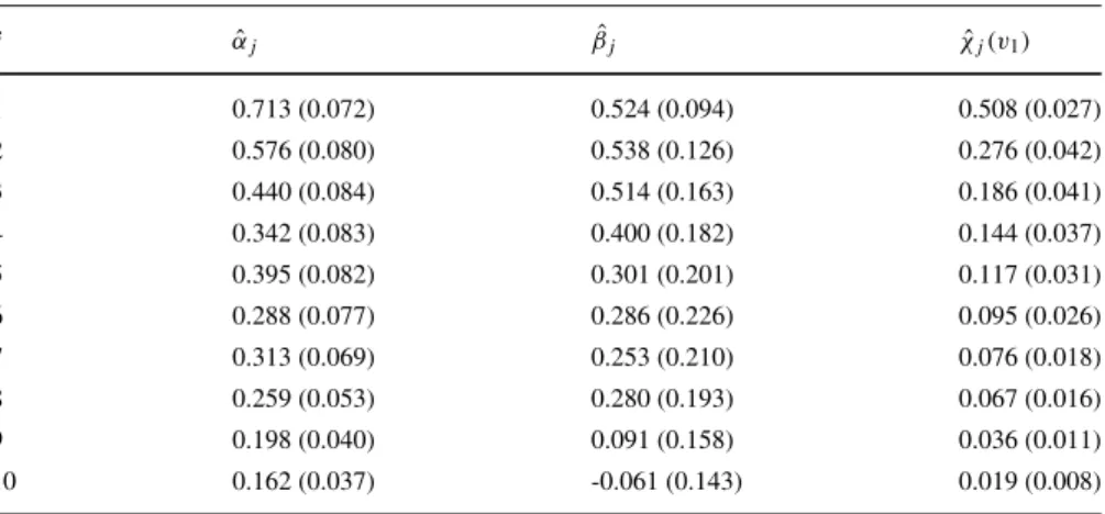
To assess if this feature is observed for the extreme events we examine the extremal dependence parameters (α1:10,β1:10). Estimation uses a threshold corresponding to
the 90 % marginal quantile, with this level being selected based on the diagnostics proposed by Heffernan and Tawn (2004). Estimates (and standard errors in parenthe-ses) of these parameters are given in Table1. These estimates are obtained without making any extremal Markov process assumptions. The estimated valuesαˆ1:10are all
statistically significantly different from one and zero, indicating the positive depen-dence form of asymptotic independepen-dence at lags 1−10. Furthermore, there is a general pattern of the values decreasing with lag, though it is not entirely monotone. The
Table 1 Estimates for the extremal dependence parameters (αj, βj) and estimated extremal dependence
measureχˆj(v1)for a set of different lag valuesj=1, . . . ,10 at the one year return levelv1. The estimates ofχj(v)are obtained from the pairwise model forXt+j|Xt. Standard errors are given in parentheses
j αˆj βˆj χˆj(v1) 1 0.713 (0.072) 0.524 (0.094) 0.508 (0.027) 2 0.576 (0.080) 0.538 (0.126) 0.276 (0.042) 3 0.440 (0.084) 0.514 (0.163) 0.186 (0.041) 4 0.342 (0.083) 0.400 (0.182) 0.144 (0.037) 5 0.395 (0.082) 0.301 (0.201) 0.117 (0.031) 6 0.288 (0.077) 0.286 (0.226) 0.095 (0.026) 7 0.313 (0.069) 0.253 (0.210) 0.076 (0.018) 8 0.259 (0.053) 0.280 (0.193) 0.067 (0.016) 9 0.198 (0.040) 0.091 (0.158) 0.036 (0.011) 10 0.162 (0.037) -0.061 (0.143) 0.019 (0.008)
ˆ
β1:10 exhibit a similar pattern. As (αˆ1:10,βˆ1:10) are often correlated it is helpful
to also consider a cluster functional estimate as the extremal dependence parame-ters combine to produce these. Here we examine the extremal dependence measure
χj(v1);j =1, . . . ,10 estimated using the unconstrained parametric estimate, where
ˆ
χj(v)is as described in Section6. Table1shows thatχˆj(v1)decreases monotonically
with increasing lag, so the pattern of dependence decay is similar for both typical and extreme values.
Figure1(right) presents the PACF for the Orleans’ daily maximum temperature data, which shows a large spike in the PACF at lag 1 with smaller values at all larger lags. This diagnostic was used by Winter and Tawn (2016) to motivate their choice of a first-order Markov model. However, there are some values of the PACF that lie outside the 95 % tolerance intervals up to lag 6. These values suggest that a first-order Markov model might omit some important higher-order structure and, as discussed in Section6, this diagnostic may miss features of the extremal process.
We wish to examine whether there is statistically significant evidence for higher-order dependence than first-higher-order for the process when in an extreme state, defined here to be when the process exceeds the 90 % marginal quantile. A hypothesis test is constructed to test whether aτth-order dependence structure provides a significantly better fit than a first-order approach. However, if the null hypothesis is rejected this only suggests that the true order of the extremal Markov process is greater than or equal to 2. The test is explained in Section6. Under a first-order model the parameters
(α2:10, β2:10)are constrained to satisfy either condition (21) or (22), whereas for
theτth-order model(α2:τ,β2:τ)are unconstrained. Tests are constructed for τ =
2, . . . ,10 and using Bonferroni bounds the significance level is set at 0.05/9. All tests for whichτ ≥7 were found to be significant at the 5 % significance level.
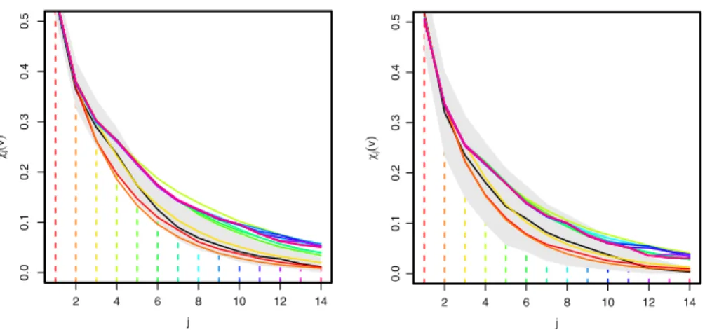
Section5set out that our main diagnostic for the selection of the order of the extremal Markov process is a comparison of estimates ofχj(v)forj ≥ 1. We have
two reference estimates to compare our extremal Markov models to: non-parametric estimatesχ˜j(v)when v is low enough that empirical estimates of χj(v) are
reli-able and the unconstrained parametric estimatesχˆj(v)for largerv. In each case we
compare these estimates withτth-order extremal Markov model estimatesχˆj(τ )(v). If the process is akth-order extremal Markov process then we should find that
ˆ
χj(k)(v)is close toχ˜j(v)for allj for lowvand toχˆj(v)for highv. Furthermore as ˆ
χ(τ2)
j (v)= ˆχ (τ1)
j (v)for allj ≤τ1< τ2,
our ability to distinguish between models of ordersτ1< τ2is only through the values
ofχˆ(τ2)
j (v)andχˆ (τ1)
j (v)forj > τ1. Consequently in the plots ofχˆ (τ )
j (v)againstj in
Fig.2we select a different colour whenj > τ.
Figure2plots these diagnostics for v corresponding to the marginal 90 % and 95 % quantiles (denoted v0.9 and v0.95). With v0.9 it appears that the third-order
scheme comes closest to the pattern observed in the empirical estimates. First- and second-order schemes seem to underestimate the strength of the dependence whereas higher-order estimates seem to lead to an overestimation, reflecting their greater vari-ation. Similar patterns are found forv0.95, although the higher-order schemes seem
2 4 6 8 10 12 14 0.0 0.1 0.2 0.3 0.4 0.5 j j v 2 4 6 8 10 12 14 0.0 0.1 0.2 0.3 0.4 0.5 j j v
Fig. 2 Estimates of the threshold dependent extremal measureχj(v)using empirical approach (black)
and different order extremal Markov chains (rainbow) withvset at 90 % (left) and 95 % (right) quantiles respectively.Greyshaded region corresponds to 95 % confidence interval for empirical obtained via a block bootstrap approach
to the increased uncertainty in the empirical estimate. Figure3shows the diagnos-tic forv = v1, which suggests that lower-order schemes are picking up the general
behaviour better, being contained with the confidence intervals at all values ofj. However, the higher-order schemes do seem to pick up some higher-order structure that is present in the original data set that is missed by a lower-order scheme. Taking all the diagnostics into account, we conclude that the third-order scheme seems to provide the most reliable estimates ofχj(v)at all levels.
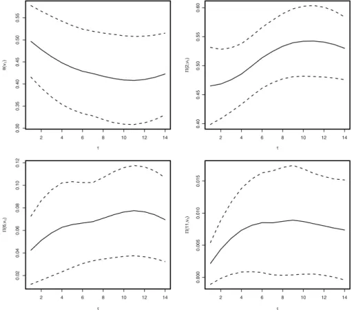
The cluster functionals that are of most importance for heatwaves areθ (v1), the
reciprocal of the mean cluster length, and(2, v1), (6, v1), (11, v1), the
proba-bilities of a cluster with at least 2, 6 and 11 exceedances ofv1. The probabilities of
Fig. 3 Estimates of the threshold dependent extremal measureχj(v1)using unconstrained parametric estimates (black) and different order extremal Markov chains (rainbow).Greyshaded region corresponds to 95 % confidence interval for unconstrained parametric approach obtained via a block bootstrap approach
2 4 6 8 10 12 14 0.0 0.1 0.2 0.3 0.4 0.5 j j v1
2 4 6 8 10 12 14 0.30 0.35 0.40 0.45 0.50 0.55 v1 2 4 6 8 10 12 14 0.40 0.45 0.50 0.55 0.60 (2,v 1 ) 2 4 6 8 10 12 14 0.02 0.04 0.06 0.08 0.10 0.12 (6,v 1 ) 2 4 6 8 10 12 14 0.000 0.005 0.010 0.015 (11,v 1 )
Fig. 4 Estimates of within cluster extremal quantities for different higher-order schemes withvset at the one-year return levelv1. Cluster functions areθ (v1), (2, v1), (6, v1)and(11, v1). Modified boot-strapping approach used to obtain 95 % confidence intervals (dotted). Estimates have been smoothed using loess method for clarity
short and long events are of particular interest as these correspond the observed dura-tions of the 2003 European heatwave at Orleans. We wish to assess the sensitivity of these cluster functional estimates to the choice of the order of the extremal process.
Figure4shows estimates of these cluster functionals for orders ofτ =1. . . ,14 for the extremal Markov model. As explained in Section6, we aim to identify the low-est order for which these cluster functionals remain constant at all higher orders, other than for sampling variability. The uncertainty bounds used in this figure are obtained via the block bootstrap. As the accurate evaluation of cluster functional is computa-tionally intensive it is not feasible to run many bootstrap replications. Instead we run a reduced number of replications to approximate the standard error for the cluster functional sampling distribution and then construct symmetric confidence intervals around the point estimate using this standard error.
The estimates of the average duration of a heatwave and the probabilities of short, median and long clusters all increase when a higher-order extremal Markov chain is used. Typically the estimates increase rapidly untilτ = 3, continue to increase
untilτ = 7 and then stabilise. However, this pattern is somewhat masked by the confidence intervals which broadly cover all estimates at all orders, so there is limited information about choice of the order. Of course we could have used a lower value of the critical level thanv1which would have been better for diagnostic purposes, but
would not have shown the sensitivity issues of the features most relevant in practice. But even at levelv1we find that for probabilities(2, v1)our diagnostic suggests
that we needτ ≥3.
Finally we focus on estimating the probability of particular cluster functionals occurring in a year. To take into account the uncertainty that we found in the selection of the order of the extremal Markov process, we compare estimates usingτ =1,3 and 7. Forτ =1 the estimated probability of observing at least one event in a year that lasts at least 2 days as 0.208 (0.200, 0.216); for 11 days the equivalent probability is 0.001 (1×10⁻⁴, 0.004), equivalent to the 1000 year return level. Whenτ =3 these estimates are 0.196 (0.171, 0.221) and 0.002 (0, 0.004) respectively. The equivalent probabilities forτ = 7 are 0.201 (0.179, 0.224) and 0.003 (0, 0.007) respectively. Thus it appears that the inclusion of higher order structure does not greatly affect the probability of smaller events but can lead to a 3-fold increase in the point estimates of the probability of very long duration extreme events. As expected, uncertainty estimates are wider for the higher-order approaches, reflecting the increased number of parameters to be estimated.
8 Discussion and conclusion
This paper provides a new framework for incorporating higher-order Markov mod-els for temporal dependence when modelling extreme events covering processes which can be either asymptotically dependent or asymptotically independent. For this purpose we have developed akth-order extremal Markov model framework for incorporating higher-order information using the conditional extremes approach of Heffernan and Tawn (2004). Such an approach is motivated by an application to heat-wave events, since all the existing time series extremes models, which have been developed under assumptions of either a first-order Markov model or that the vari-ables are asymptotically dependent, do not adequately capture the properties we observe for heatwaves.
Our results show that using standard time series diagnostics to identify the order of an extremal Markov process can lead to errors when interest is restricted to the extremes of the process. This necessitated the development of a range of new diag-nostics for choosing the ‘best’ order scheme to use for extreme events. Specifically, in our example the use of standard time-series diagnostics ignored structure in the extremes which leads to the underestimation in the probability of longer and poten-tially devastating heatwave events. One area for further work is to formalise and unify our range of heuristic diagnostic methods for estimating the order of the extremal Markov process. To help achieve this a systematic study of the performance of these methods in a simulation study is needed. This study should cover both asymptotically independent and asymptotically dependencekth-order Markov processes, each with varying strengths of dependence.