On the relevance of modeling volatility for pricing purposes

(1)

First version: September 1997 This version: October 1999

On the Relevance of Modeling Volatility for Pricing Purposes Manuel Moreno3

Department of Economics and Business Universitat Pompeu Fabra

Carrer Ramon Trias Fargas, 25-27 08005 Barcelona, Spain.

phone: (34-93) 5.42.27.71 fax: (34-93) 5.42.17.46

This paper presents a two-factor (Vasicek-CIR) model of the term struc-ture of interest rates and develops its pricing and empirical properties. We assume that default free discount bond prices are determined by the time to maturity and two factors, the long-term interest rate and the spread. As-suming a certain process for both factors, a general bond pricing equation is derived and a closed-form expression for bond prices is obtained. Em-pirical evidence of the model's performance in comparisson with a double Vasicek model is presented. The main conclusion is that the modeling of the volatility in the long-term rate process can help (in a large amount) to t the observed data can improve - in a reasonable quantity - the prediction of the future movements in the medium- and long-term interest rates. However, for shorter maturities, it is shown that the pricing errors are, basically, negligible and it is not so clear which is the best model to be used.

Keywords: Term Structure of Interest Rates, Bond Pricing Equation, Two-Factor Models, Ornstein-Uhlenbeck Process, CIR Process.

(2)

The evolution over time of interest rates for default-free zero-coupon bonds is a topic that has been extensively analyzed in the nancial literature. Initially, the analysis of this evolution was performed by means of one-factor models which assume that movements in interest rates are driven by changes in the short-term (instantaneous) riskless interest rate (see, among others, Vasicek (1977), Cox et al (1985) or Chan et al (1992)). However, it is now widely ac-cepted that interest rates are aected by more than one state variable. In this direction, several papers as Richard (1978), Brennan and Schwartz (1979), Schaefer and Schwartz (1984), Cox et al (1985), Longsta and Schwartz (1992), Due and Kan (1996), Chen (1996), Dai and Singleton (1997) and Boudoukh et al (1999) use multiple factors to explain the future movements that interest rates may show.

There is substantial empirical evidence1 _{that shows that movements in}

interest rates can be decomposed in three types of \basic" changes related to the level of interest rates, the slope, and the curvature of the yield curve. As the curvature is usually the less important explanatory variable when dealing with spot interest rates, we can think that movements in spot interest rates may be reasonably well explained by the two rst factors.

In fact, this is the motivation for the model previously presented and developed in Moreno (1996) which uses the long-term interest rate and the spread of interest rates as state variables (that is, the dierence between the long-term interest rate and the short-term interest rate is used as a rough measure of the slope of the yield curve). In that paper, both factors are assumed to follow a Vasicek process and, therefore, both variables (1) show mean reversion to a certain long term value and (2) their diusions reect a constant variance term. Under these assumptions, a general bond pricing equation was derived and a closed-form expression for zero-coupon bond and for interest rate derivatives prices was computed, This paper also presented the empirical performance of this model in relation to an alternative one-factor model.

It can be argued that one of the assumptions made in Moreno (1996), namely, the constant variance in the diusion of the processes followed by

a

1_{See, for instance, Jones (1991), Litterman and Scheinkman (1991), Zhang (1993) and} Knez, Litterman, and Scheinkman (1994).

(3)

both factors is too restrictive from an empirical point of view.2 _This

restric-tive feature leads to the present paper whose main objecrestric-tive is to analyze if modeling the volatility improves the empirical performance of the Moreno (1996) model. Thus, the same state variables will be used although we will assume that the long-term interest rate does not follow a Vasicek process but a root-square (CIR-type) process. This alternative model will be de-noted hereafter as the Vasicek-CIR model and it can be considered, from a theoretical point of view, as an special case of the Schaefer and Schwartz (1984) model.

The schedule of this paper is as follows. Section 2 presents the main as-sumptions of the Vasicek-CIR model and provides the basic pricing equation that any derivative asset must satisfy. This equation, with the appropriate terminal condition, allows us to obtain the price of any asset that, at ma-turity, pays a certain payo as indicated in such terminal condition. In this section we (a) compute the analytical expression that indicate the price of any discount bond under the assumptions given by this two-factor model and (b) recall the analogous formula that was obtained in Moreno (1996) (Vasicek-Vasicek model hereafter). Section 3 analyzes the empirical behav-ior of both models by comparing the usefulness of these alternative formulas to t and forecast bond prices, that is, the in- and out-of-sample performance of such expressions. The data analyzed correspond to Spanish interest rates and bond prices for dierent maturities during the period 1991-1995. Finally, Section 4 summarizes and concludes.

In this section we present the two-factor (Vasicek-CIR) model that we will use to price default-free discount bonds by deriving (and solving) the pricing equation which must be veried by the prices of these bonds.

The main assumption of this model is that the price, at time t, of a default-free discount bond that pays $1 at maturity T depends only on the current values of two state variables and time to maturity, = T 0 t. The

a

2_{Interest rate volatility is usually increasing in interest rate level although there is no} consensus about the exact relationship between volatility and level. See Chan et al (1992), At-Sahalia (1996), Conley et al (1997) and Stanton (1997) for this issue.

(4)

main motivation for the factors to be used is the empirical evidence (see footnote 1) that changes in interest rates are a combination of movements in (a) the level of interest rates, (b) the slope and (c) the curvature of the yield curve, which eect is usually negligible. Therefore, we can use the long-term rate and the spread as the variables that help us to explain the movements in the general level of interest rates and changes in the relationship between the short and the long end of the yield curve. With both variables, we can also try to explain the intermediate movements of the yield curve.3

Although most previous studies use the short-term interest rate as one of the state variable, we redene these variables and, analogously to Schaefer and Schwartz (1984), the factors to be used are the long-term rate, denoted by L, and the spread, denoted by s, the dierence between the long- and the short-term rate, denoted by r. This selection of state variables allows us to use the assumption of orthogonality between them.4

Once chosen these variables, we assume that their evolution over time is given by the following stochastic dierential equations5_:

(

ds = 1(s; L)dt + 1(s; L)dw1

dL = 2(s; L)dt + 2(s; L)dw2 (1)

where t denotes calendar time, and dw1 and dw2 are standard Brownian

processes where E[dw1] = E[dw2] = 0, dw12 = dw22 = dt, and (by the

orthog-onality assumption) it is veried that E[dw1dw2] = 0. 1(:) and 2(:) are the

expected instantaneous rates of change in the state variables and 2

1(:) and

2

2(:) are the instantaneous variances of changes in these factors.

Let P (s; L; t; T ) P (s; L; ) be the price, at time t, of a default-free discount bond that pays $1 at maturity T = t + . We can express the instantaneous percentage change in the price of this bond as the sum of its expected rate of return and the unexpected variations in return due to the

a

3_{Two alternative couples of factors to be used may be: (a) the long-term interest} rate and the short-term interest rate and (b) the short-term interest rate and the spread. However, the above two variables are chosen because of a better analytical tractability.

4_{This assumption simplies the analytical tractability of the model. Empirical evidence} that supports this assumption can been seen in Ayres and Barry (1980), Schaefer (1980), Nelson and Schaefer (1983) and, for the Spanish case, in Moreno (1996).

5_{After presenting this generic model and deriving the general pricing equation, we will} particularize it to obtain the Vasicek-CIR model

(5)

random changes in the factors dP (s; L; t; T )

a

P (s; L; t; T ) = (s; L; t; T )dt + s1(s; L; t; T )dw1+ s2(s; L; t; T )dw2 (2) The steps to be given to obtain the bond pricing equation are very standard6 _{and can be summarized as follows:}

1. Application of It^o's Lemma

2. Setting up of a (hedging) portfolio, composed of three bonds with dif-ferent maturities, that is instantaneously riskless

3. Under no-arbitrage conditions, the expected rate of return of this port-folio must equate the instantaneous riskless rate of interest

These three steps jointly with a little algebra lead us to the following partial dierential equation

1

a

2[21(:)Pss+ 22(:)PLL] + [1(:) 0 1(:)1(:)]Ps

+[2(:) 0 2(:)2(:)]PL+ Pt0 rP = 0 (3)

where subscripts denote partial derivatives. The coecients 1(:) and 2(:)

can be interpreted as the market prices of the spread and long-term rate risk, respectively.

Therefore, given the stochastic process (1) we have assumed for both vari-ables, (3) is the fundamental equation for the pricing of default-free discount bonds of dierent maturities which depend solely on the spread, the long-term interest rate, and its time to maturity. In this equation we deal with the market prices of risk, i(:), because the only way to tie down the bond

prices in our (partial equilibrium) model is by means of these (exogenous) parameters.

The solution of the equation (3), subject to the terminal condition given by the nal payment of the bond, P (s; L; 0) = 1; 8 s; L, is the price of the discount bond we are looking for.

a 6_{For more details, see Moreno (1996).}

(6)

The coecients of the bond pricing equation (3) are the parameters of the stochastic process (1) which was assumed for the two factors and the market prices of the risk related to both state variables. As this equation is too general to be solved analytically, we will make the following assumptions about these coecients:

Assumption 1 The market price of the spread risk is linear in this variable, that is

1(:) = a + bs

Assumption 2 The market price of the long-term rate risk is proportional to the square root of this variable, that is

2(:) = d

pa

L

Assumption 3 Each of the state variables follow a diusion process

(

ds = k1(10 s)dt + 1dw1

dL = k2(20 L)dt + 2

pa

Ldw2 (4)

The motivation for the rst two assumptions is that a constant market price of risk is too restrictive and quite unrealistic. The rst assumption is the generalization of the one presented in Vasicek (1977) while the second one is similar to the one obtained in Cox et al (1985). Regarding the third assumption, the rst process, known as Ornstein-Uhlenbeck process, has been used previously by Vasicek (1977) while the second one was proposed in Cox et al (1985). Both processes show mean reversion, an important stylized fact that interest rates usually show. In the process assumed for the spread, we nd a constant variance in the diusion term while the variance of the long-term rate is proportional to its level. For each state variable, ki > 0 is the

coecient of mean reversion which reects the speed of adjustment of the variable towards its long-run mean value, i, and dwi are standard Brownian

motions.

Under these three assumptions, we can rewrite the equation (3) as 1

a

212Pss+ q1(^10 s)Ps+1a

(7)

subject to the terminal condition

P (s; L; 0) = 1; 8 s; L (6)

where

q1 = k1+ b1; ^1 = (k11 0 a1)=q1

q2 = k2+ d2; ^2 = k22=q2

Solving the partial dierential equation (5) we obtain the following propo-sition:

Proposition 1 The value at time t of a discount bond that pays $1 at time T , P (s; L; t; T ) P (s; L; ), is given by P (s; L; t; T ) = A()e0B()s0C()L ₍₇₎ where = T 0 t and A() = A1()A2() A1() = exp ( 0a12 4q1B 2_{() + s}3_{(B() 0 )} ) A2() = 2 4 2 exp n (q2+ )a 2 o a (q2+ ) expfg + ( 0 q2) 3 5 2k22=₂2 (8) B() = 1 0 ea0q1 q1 C() = a2(expfg 0 1) (q2+ ) expfg + ( 0 q2) with q1 = k1+ b1; ^1 = (k110 a1)=q1; s3 = ^10 12=(2q12) q2 = k2+ d2; ^2 = k22=q2; = qa q2 2 + 222 (9)

(8)

The terms in equation (8) verify

0 < Ai() < 1; 8 > 0; Ai(0) = 1; Ai(1) = 0; i = 1; 2

0 < B() < ; 8 > 0; B(0) = 0; B(1) = 1=q1 (10)

0 < C() < ; 8 > 0; C(0) = 0; C(1) = 2=(q2 + )

Substituting t = T into (7), it is shown that the terminal condition for the price bond, P (s; L; 0) = 1; 8 s; L, is satised. Moreover, it is also derived that

P (0; 0; ) = A() = A1()A2() < 1; 8 > 0

It can be checked that the following realistic features are veried lim

s!1P (s; L; ) = limL!1P (s; L; ) = lim!1P (s; L; ) = 0

that is, when any of the arguments included in the bond price formula tends to innity, the price converges to zero. It is also easily shown that the bond price function is decreasing and convex in both factors and decreasing with the time to maturity.

Once we have obtained the expression (and properties) for the bond price formula under the Vasicek-CIR model, we will recall the assumptions made in Moreno (1996) and the corresponding pricing formula that was derived in that paper:

Assumption 1' (equal to Assumption 1) The market price of the spread risk is linear in this variable, that is

1(:) = a + bs

Assumption 2' The market price of the long-term rate risk is linear in this variable, that is

2(:) = c + dL

Assumption 3' Each of the state variables follow a diusion process of Vasicek type ₍

ds = k1(1 0 s)dt + 1dw1

dL = k3(3 0 L)dt + 3dw3 (11)

Under these assumptions, we can rewrite the equation (3) as 1 a 212Pss+ q1(^10 s)Ps+ 1 a 232PLL+ q3(^30 L)PL+ Pt0 (L + s)P = 0 (12)

(9)

where

q1 = k1+ b1; ^1 = (k11 0 a1)=q1

q3 = k3+ d3; ^3 = (k330 c3)=q3

The solution of the dierential equation (12), subject to the terminal condition given by the payo of the bond at maturity (see equation (6)), was established in the following proposition:

Proposition 2 (Proposition 1 in Moreno (1996)) The value at time t of a discount bond that pays $1 at time T , P (s; L; t; T ) P (s; L; ), is given by P (s; L; ) = D()e0E()s0F ()L ₍₁₃₎ where = T 0 t and D() = D1()D3() D1() = exp ( 0a12 4q1B 2_{() + s}3_{(B() 0 )} ) D3() = exp ( 0a32 4q3C 2_{() + L}3_{(C() 0 )} ) (14) E() = 1 0 ea0q1 q1 F () = 1 0 ea0q3 q3 with q1 = k1+ b1; ^1 = (k110 a1)=q1; s3 = ^1 0 21=(2q21) q3 = k3+ d3; ^3 = (k330 c3)=q3; L3 = ^3 0 23=(2q32) (15)

Proof: It is similar to the proof of Proposition 1 and it is omitted for the sake of brevity.

(10)

In this section, we describe the empirical application in which we compare the tting and forecasting behavior of the Vasicek-CIR and the Vasicek-Vasicek models. This comparison is performed analyzing the in- and out-of-sample properties of both models. The dataset consists of daily Spanish interest rates and zero-coupon bond prices and cover the period 1991-1995.7

For each day of this period, we have interest rates (in annualized form) and bond prices for ten dierent maturities: 1, 7, and 15 days, 1, 3, and 6 months, and 1, 3, 5, and 10 years. The interest rates corresponding to the shortest and longest maturity (1 day / 10 years) are used as proxies of the short- and long-term interest rate, respectively.

The main descriptive characteristics of the state variables used in both two-factor models are:

1. For both interest rate series, the unconditional average is larger than 10%. Short-term interest rates are larger than this mean value until October 1993 while the long-term interest rates exceed this level in the whole period except from June 1993 through June 1994. On the other hand, the spread has a mean value very close to zero and ranges between 04% and 8%.

2. The short-term rate is more volatile and moves into a wider interval than long-term rates do.

3. Both state variables show an uniformly high degree of serial correlation. 4. Most of the changes in the short-term interest rates are smaller than 100 basis points while changes in long-term rates are much smoother. As a consequence, changes in the spread are quite similar to changes in short-term interest rates.

5. It is seen a small decrease - in mean - in interest rates through the sample period.

6. Evidence of mean reversion in spread and interest rates is derived.

a

7_{For more details on these data, see Nu~nez (1995) for technical details on the procedure} used by the Bank of Spain to estimate them and Moreno (1996) for a descriptive and graphical analysis.

(11)

7. The theoretical assumption about the orthogonality between the state variables is empirically corroborated.

Next we present the empirical performance of both models. We recall that both models use the same factors and the main dierence between them derives from the alternative processes assumed for the long-term rate, L.

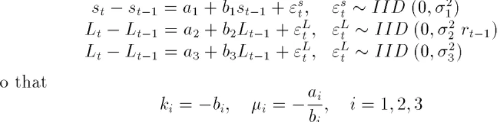
Each state variable of the two competing models, s and L, follows a diu-sion process (see equations (4) and (11)). The diudiu-sion parameters of these processes (ki; i; i; i = 1; 2; 3) are estimated by the Generalized Method

of Moments presented in Hansen (1982)8_{. The econometric specication in}

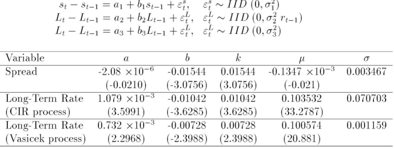
discrete time is st0 st01 = a1+ b1st01+ "st; "st IID (0; 12) Lt0 Lt01 = a2+ b2Lt01+ "Lt; "Lt IID (0; 22 rt01) Lt0 Lt01 = a3+ b3Lt01+ "Lt; "Lt IID (0; 23) so that ki = 0bi; i = 0aai bi; i = 1; 2; 3

Table I includes the estimation results obtained for the sample period 1991-1995 and shows that the parameters bi of the discrete time specication

(and hence, the diusion parameters ki) are signicantly dierent from zero.

So, there is evidence of mean reversion in all the state variables.

In both models, the long-term interest rate tends to a mean value close to 10% while the spread tends to a mean value close to zero. Comparing the two processes assumed for the long-term rate, it may be interesting to recognize that, under the CIR model, the long rate reverts faster to its long-term value than when considering the Vasicek assumption.

After estimating the parameters of the diusion processes followed by the factors in both models, these values are used to obtain the remaining parameters of equations (7) and (13). Thus, similarly to Moreno (1996), we use the specications

P = P (q1; q2; s3jk1; k2; 1; 2; 1; 2; s; L; ) + "

P = P (q1; q3; s3; L3jk1; k3; 1; 3; 1; 3; s; L; ) + " (16)

a

8_{For details on this technique and its applications in the estimation of continuous-time} models, see Moreno and Pe~na (1996).

(12)

where P is the observed price of the discount bonds available at time t, P (:) is the closed-form pricing equation for each model (see equations (7) and (13)) and " is an error term.

The parameters of the equations (16) (qi; i = 1; 2; 3; s3; L3) are estimated

on a daily basis for the period 1991-1995 by means of a panel of data where we have daily yield curves containing a cross-section of discount bond prices. Therefore, we have a matrix with 1230 rows and 10 columns where each row includes the (ten) zero-coupon bond prices available at each day and each column contains the bond prices for a certain maturity.

We estimate the non-linear equations (16) for each day of the period 1991-1995. The estimation of the rst equation provides the parameters of the Vasicek-CIR model (that is, q1; q2; s3) while the estimation procedure,

when applied to the second equation, provides the parameters of the Vasicek-Vasicek model, that is, q1; q3; s3; L3.

Estimation results for the daily parameters of the Vasicek-CIR model are included in Table II.9 _{This table shows the average of the estimated}

parameters obtained for (a) the full sample period and (b) the sample period divided year by year and reects that all the parameters are positive and highly signicant.

The evolution over time of these parameters can be seen graphically in Figure 1. This gure shows that the highest values are attained in 1991 while the lowest (and more stable) parameters correspond to the period 1994-1995. In the next step, we can compute the values, day by day, of the market prices of risk related to each state variable using the estimated parameters obtained from equation (16) jointly with the expressions (9) and (15) and the Assumptions 1 and 2. A graphical representation of these values, for the Vasicek-CIR model, can be seen in Figure 2. The average values of these prices - under both models - for the whole period and for every year, are included in Table III.

Analyzing the two factors of the Vasicek-CIR model, both market prices of risk are highly signicant and have a similar behavior across the period 1995: each price has always the same sign during all the period 1991-1995 (for the long-term rate, the market price of risk is always positive and

a

9_{We do not show the results for the Vasicek-Vasicek model that can be seen in Table} VIII in Moreno (1996). That paper provided all the results for the Vasicek-Vasicek model that are included in the following tables in this paper.

(13)

the risk related to the spread has always a negative price) and both series of market prices are specially low in 1992 and the second half of the period 1991-1995. In absolute terms, the price of the spread risk is, at every moment, much higher than the price of risk of the long-term rate.

On the other hand, for the Vasicek-Vasicek model, we can observe a very dierent behavior between both factors and with respect to the alternative model. Thus, the two basic features for the prices of risk in this model are:

1. For the full period, the market prices of risk for both state variables are positive and signicantly dierent from zero.

2. Analyzing this period year by year, the parameters are also signicantly dierent from zero but they show a changing sign. Thus, the mean market price of risk of the spread is negative in the last two years of the sample period while the average of the market price of risk related to the long-term rate is negative in 1991-1992 and 1994.

Finally, we will use the values of the diusion parameters jointly with the parameters estimated by means of the equation (16) to analyze the tting and forecasting power of both two-factor models. The within- and out-of-sample periods are 1991-1994 and 1995, respectively.

First, the in-sample estimated data, for each day of the period 1991-1994 and for both models, are provided by the inclusion of the (daily) estimated parameters and the estimated parameters of the diusion processes in the non-linear equation (16).

Next, we will compare the out-of-sample properties of both models by using the k-step-ahead forecasts that are generated for the bond prices. These t + k-time forecast values are built using the coecient estimated from time t. This procedure is repeated for each day of 1995.

Once obtained the in- and of-sample forecasts, the (within and out-of-sample) pricing errors of both models are computed to compare one each other. Thus, we dene, for time t, the error, et, and the percentage error,

P Et, as

et= Pt0 ^Pt; P Et= Pat0 ^Pt

Pt 2 100

where Pt and ^Pt are, respectively, the observed and the estimated (tted or

(14)

For both models, the within-sample (absolute and percentage) pricing errors are shown in Figures 3 and 4. For all the maturities, it can be seen that the Vasicek-Vasicek model provides a very large pricing error in May, 1993. This error coincides with a sharp change in the short-term rate and in the spread. For both models, neither gure suggests a systematic pattern in these pricing errors.

Denoting by N the number of days of the period to be analyzed, we use the pricing errors to compute several accuracy measures that help us to compare the empirical performance of both models:

1. Mean Error (ME). This measure weights equally the daily errors. Therefore, positive values can be oset with negative values and, thus, this measure may be small even with large errors. Its expression is

ME = a1 N N X t=1et= 1 a N N X t=1(Pt0 ^Pt)

2. Mean Absolute Error (MAE). As the mean error, this measure gives an equal weight to the daily errors but positive and negative errors do not cancel out. It is dened as

MAE = a1 N N X t=1jetj = 1 a N N X t=1jPt0 ^Ptj

3. Root Mean Squared Error (RMSE). It is usually the most common measure of accuracy and its denition is

RMSE = v u u t a 1 a N N X t=1(et) 2 ₌ v u u t a 1 a N N X t=1(Pt0 ^Pt) 2

4. Mean Percentage Absolute Error (MAPE) Similarly to the mean absolute error, the absolute value of the error is used but each error is weighted by the current value of the bond price. Its expression is

MAP E = a1

N

N X t=1jP Etj

(15)

5. Root Mean Squared Percentage Error (RMSPE). This measure is similar to the root mean squared error but, similarly to the MAPE, the daily errors are weighted by the actual bond prices. It is given by

RMSP E = v u u t a 1 a N N X t=1(P Et) 2

These ve descriptive measures, for both models, are computed for 1991-1994 (within sample period), for 1995 (out-of-sample period) and for dierent subperiods. The within and out-of-sample results are reported in Tables IV-VI and Tables IV-VII-X, respectively.

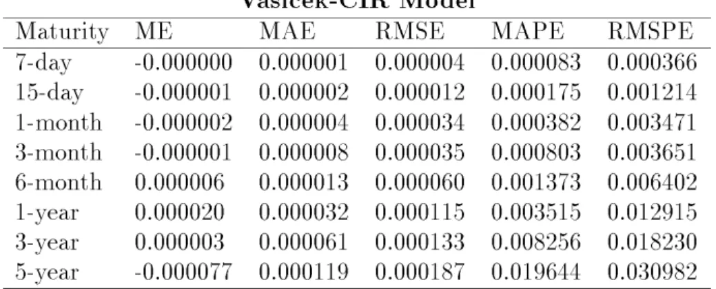
The performance of both models, for the within-sample period, is included in Table IV. For this period, the Vasicek-Vasicek model underprices the short-and medium-term bonds short-and overprices the bonds whose maturity is beyond one year. On the other hand, the Vasicek-CIR model overprices the bonds with maturities up to three months as well as the 5-year bonds.

All the statistics included in Table IV reect that both models provide a very big accuracy to the observed bond prices for all the maturities. It can be seen that the pricing errors are increasing with the maturities (the longer the maturity, the larger the error price) but the MAPE for the Vasicek-Vasicek and the Vasicek-CIR models is smaller than 0:26% and 0:02%, respectively. Moreover, in the Vasicek-CIR (Vasicek-Vasicek) model, this statistic is always smaller than 0:01% (0:08%) except for the 5-year bond price.

Comparing both models, the CIR model outperforms the Vasicek-Vasicek model for all maturities and for all the statistics. In short-term bonds, with maturities smaller than one month, both models provide negli-gible errors and the improvement obtained with the Vasicek-CIR model over the other one is not very large.

On the other hand, focusing on the maturities beyond one month, the CIR model provides a huge improvement: the errors from the Vasicek-Vasicek model are decreased in more than 88% for all these maturities. The biggest improvement in accuracy is achieved in the medium-term maturities (six month and one year) and in 5-year bonds, maturity in which the error measures from the Vasicek-CIR model are about 6% of the error measures provided by the Vasicek-Vasicek model. This conclusion is obtained for all the statistics.

(16)

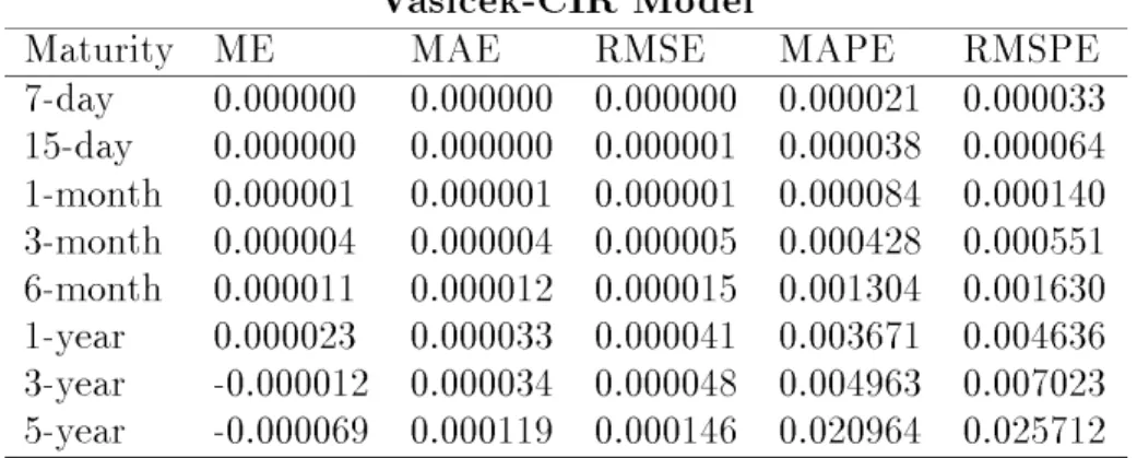
Table V includes the results obtained for the year 1992. Similarly to the period 1991-1994, the Vasicek-Vasicek model underprices the shortest maturities (up to six months). In contrast to what happened in the whole within-sample period, this underpricing can also be seen in the Vasicek-CIR model which, on the other hand, overprices the bonds that mature beyond one year.

In this year, both models t the observed data specially well. Thus, the error measures for both models are decreased in more than half for most of the maturities with respect to the whole period. Comparing both models, the error measures of the Vasicek-CIR model, as in the whitin-sample period, are about 10% of the statistics provided by the Vasicek-Vasicek model for all the maturities longer than 15 days.

Therefore, the main conclusion for this year is the same than the obtained for the period 1991-1994: for the shortest maturities, both models t specially well to the data but, for most of the remaining maturities, the Vasicek-CIR model provides a remarkable large improvement in accuracy.

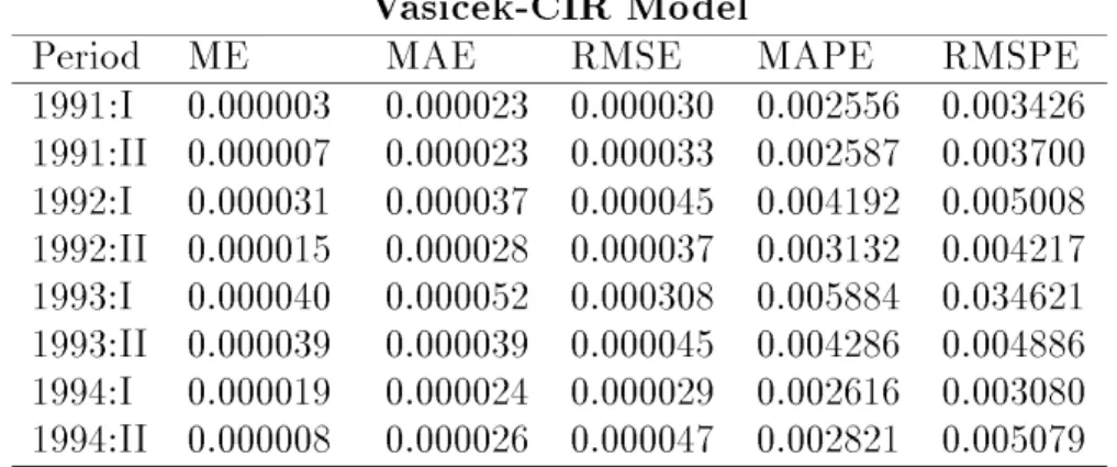
Several subperiods have been analyzed and, basically, the same conclu-sions are reached. For illustrative purposes, Table VI includes the whitin-sample results obtained for 1-year bonds for each semester of the period 1991-1994.

Looking at every statistic, it is shown that the Vasicek-CIR model ts better than its competing model in all the semesters and it works specially well in 1991 and 1994 while the Vasicek-Vasicek model obtains its best per-formance in the rst semester of 1992 and in the second one of 1994.

Based on a mean absolute error (MAE or MAPE) criterion, the superi-ority of the Vasicek-CIR model implies an improvement of about 90% in all the semesters but the last one in which the errors from the Vasicek-Vasicek model are decreased in 'just' 77%.

For all the semesters, the mean absolute percentage error of the Vasicek-CIR model is around 0:003% that is about fteen times smaller than the obtained for the Vasicek-Vasicek model. This superiority is specially re-markable in the second semester of 1991 and in the rst one of 1994 when the absolute value of the errors are decreased in more than 96%.

The forecasting power of both models is analyzed by computation of one-and ve-step ahead forecasts10_{of bond prices for every maturity and for every}

a

(17)

day of the year 1995. Measures of the forecasting pricing errors are included in Tables VII-X.

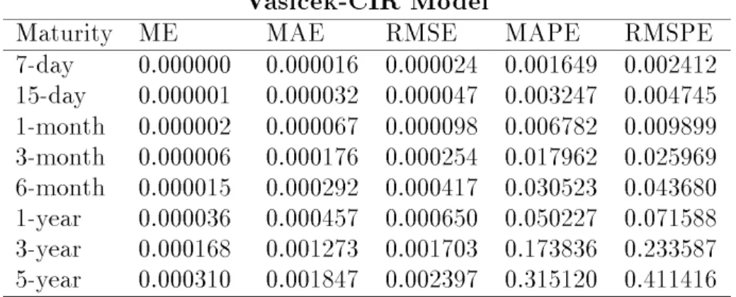
Tables VII-VIII include the measures for one-step-ahead forecasts. Thus, Table VII provides the one-step-ahead measures for the whole out-of-sample period. It can be seen that (1) both models forecast quite well, (2) the fore-casting power decreases with the time to maturity, and (3) for both models, the MAPE (RMSPE) is always smaller than 0:36% (0:48%). It can also be seen that both models perform similarly for the shortest maturities and, in fact, the Vasicek model performs slightly better than the Vasicek-CIR model.

For maturities beyond one month, the Vasicek-CIR model forecasts better than the Vasicek-Vasicek model showing that the modeling of the volatility in the long-term rate process helps to predict the movements in the medium-and long-term interest rates.

This superior forecasting performance is not monotonic in the time to maturity. Thus, the largest improvement is obtained in the 1-year bond prices when the error measures from the Vasicek-Vasicek model are decreased in more than 21% (15%) when working on a (root) mean absolute criterion. In the remaining bonds, the improvement in the relative forecasting power is much smaller (2 0 7%) and never exceeds 12%, value that is obtained when forecasting the 5-year bonds.

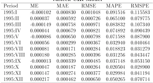
Table VIII provides the error measures obtained, for every month of 1995, from 1-year bonds in which the Vasicek-CIR model achieves its best relative performance. Both models perform better in the second semester (with a MAPE (RMSPE) smaller than 0:06% (0:08%)) than in the rst one, when the MAPE (RMSPE) reaches 0:1% (0:12%). It can also be seen a similar behavior in both models from January to April (with a small superiority of the Vasicek-Vasicek model in this period) and in the two last months of 1995. In the period May-October, the Vasicek-CIR model achieves an improvement of the out-of-sample performance that ranges between 20% (in May) and 65% (in July).

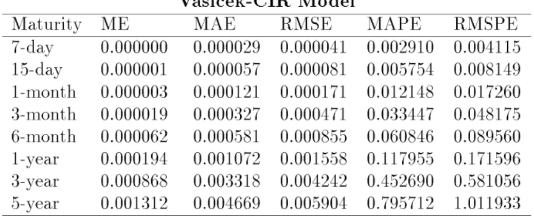
Finally, Tables IX-X show the results obtained when the forecasting hori-zon is ve days. Thus, Table IX includes the measures obtained with the out-of-sample errors for all the maturities in 1995. Although these measures are bigger than in the shorter forecasts, they are reasonably small as reected in the MAPE or the RMSPE that are, for both models, smaller than 0:8% and 1%, respectively.

(18)

The results are analogous to the obtained with the previous predictions: (1) the forecasting power decreases with time to maturity, (2) the Vasicek-Vasicek model outperforms its rival model in the maturities smaller than six months, and (3) the Vasicek-CIR forecasts better than the Vasicek-Vasicek model in the maturities beyond six months. However, this improvement is usually quite small (between 1% and 3%) and only increases until 5% when forecasting 1-year bond prices.

The last table provides the quarterly results obtained with ve-step-ahead forecasts for 1- and 5-year bonds. In both maturities, it can be seen a better forecasting behavior in the second half of 1995 than in the rst one. For 1-year bonds, both models show a MAPE smaller than 0:2% in all the quarters and the Vasicek-CIR model outperforms the Vasicek-Vasicek model whose error measures are decreased between 5% and 15% in the period April-September. Focusing on the forecasting errors for 5-year bond prices, the MAPE statistic ranges between 0:6% and 1%. In this case, the Vasicek-CIR model improves the forecasts from its competing model in 10% from July to Septem-ber and, in the remaining quarters, its improvement is much smaller (102%).

This paper has presented a two-factor (Vasicek-CIR) model in continuous time for the analysis of the terms structure of interest rates and its empirical behavior has been analyzed with respect to a second alternative model. The main common characteristic of these two models is that both employ the same factors (state variables) to explain the unexpected changes that interest rates may show in the future. These factors are the long-term interest rate and the spread, the dierence between the long- and the short-term interest rate. The Vasicek-CIR model assumes that the spread follows a Vasicek process while the long-rate is modeled as a CIR-type process. On the other hand, the Vasicek-Vasicek model has assumed that both variables follow a Vasicek process. This second model was previously presented Moreno (1996) which also developed its pricing properties, the implications on the term structure of interest rates and analyzed its empirical properties with a sample of daily interest rates and bond prices that cover the period 1991-1995.

(19)

performance of both models in the period 1991-1995. Therefore, we can determine if modeling the volatility of the long-term interest rate may help us to explain the future movements of interest rates. As a starting point, we have derived a bond pricing equation whose solution indicates the price of a zero-coupon bond under certain assumptions, namely, this price depends solely on the current values of two state variables (mentioned above) and the time to maturity of the bond.

After this solution is obtained, it is used to analyze the tting and fore-casting properties of this model. These properties are, in a posterior stage, compared with the ones derived from the Vasicek-Vasicek model. The pa-rameters of our competing models have been estimated in two steps. In the rst one, the parameters of the diusion processes have been estimated by the Generalized Method of Moments by Hansen (1982). Once these values are obtained, the remaining parameters are estimated by using a cross-section technique. As a result of this combination of estimation methods, we have been able to obtain the daily market prices of risk corresponding to both state variables for both models.

Thus, it has been shown that, for the Vasicek-CIR model, these prices are highly signicant and have a constant sign during all the period 1991-1995. On the other hand, under the Vasicek-Vasicek model, it can be seen that the market prices of risk are signicantly dierent from zero and positive for 1991-1995 although they show a changing sign when analyzing yearly this period.

Finally, we have analyzed the tting and forecasting power of both mod-els. The within- and out-of-sample periods are 1991-1994 and 1995, respec-tively. After computing the within- and out-of-sample forecasts, the pricing errors of both models (and several accuracy measures) for dierent subperi-ods have been obtained to compare one each other.

All these statistics show the following facts: (1) both models provide a very big accuracy to the observed bond prices for all the maturities, (2) the pricing errors are increasing with the maturities, (3) the MAPE for the Vasicek-Vasicek and the Vasicek-CIR models is smaller than 0:26% and 0:02%, and (4) in the Vasicek-CIR (Vasicek-Vasicek) model, this statistic is always smaller than 0:01% (0:08%) except for the 5-year bond price.

Comparing both models, it can be seen that (1) the Vasicek-CIR model outperforms the Vasicek-Vasicek model for all maturities and for all the statistics, (2) in maturities smaller than one month, both models provide

(20)

negligible errors and the relative improvement obtained with the Vasicek-CIR model is not very large, (3) dealing with maturities greater than one month, the errors from the Vasicek-Vasicek model are decreased in more than 88% for all these maturities, (4) the biggest improvement (about 90 0 94%) in accuracy is achieved in the medium-term maturities and in 5-year bonds. Several subperiods have been analyzed and the same conclusions are reached. The forecasting power of both models has been analyzed by one- and ve-step ahead forecasts for every maturity and for every day of the year 1995. Looking at one-step-ahead forecasts, it has been shown that - similarly to the within-sample period - both models perform quite well, the forecasting power decreases with the time to maturity and, for the shortest maturities, both models perform similarly. However, for maturities beyond one month, the Vasicek-CIR model forecasts better than the Vasicek-Vasicek model although this superior forecasting behavior is not monotonic in the time to maturity. Thus, the best relative performance is obtained in the 1-year bond prices when the error measures from the Vasicek-Vasicek model are decreased in more than 21%. In the remaining bonds, the improvement is much smaller ranging between 2% and 12%.

Finally, dealing with ve-step-ahead forecasts, all the statistics reect a worse performance than in the previous (shorter) forecasts although similar results are shown: (1) the forecasting power decreases with time to maturity, (2) the Vasicek-Vasicek model outperforms its rival model in the shortest maturities and (3) the Vasicek-CIR forecasts better than the Vasicek-Vasicek model in the maturities beyond six months. In this case, this improvement is usually quite small, between 1% and 5%.

Therefore, the main conclusion is that the modeling of the volatility in the long-term rate process can help (in a large amount) to t the observed data can improve - in a reasonable quantity - the prediction of the future movements in the medium- and long-term interest rates. However, for shorter maturities, it has been shown that the pricing errors are, basically, negligible and it is not so clear which is the best model to be used.

(21)

Appendix: Proofs

Proof of Proposition 1

The method of the separation of variables allows us to write the solution of the equation (5) subject to (6) as

P (s; L; t; T ) = X(s; t; T ) Z(L; t; T ) (17) where X(s; t; T ) solves the equation

1

a

212Xss+ q1(^10 s)Xs+ Xt0 sX = 0 (18) subject to the terminal condition

X(s; T; T ) = 1; 8 s (19)

and Z(L; t; T ) is the solution of the equation 1

a

222LZLL+ q2(^20 L)ZL+ Zt0 LZ = 0 (20) with terminal condition

Z(L; T; T ) = 1; 8 L (21)

To solve equation (18), we posit a solution of the type

X(s; t; T ) = X(s; ) = A1()e0B()s (22)

Hence, the equation (18) becomes 1 a 221B2() 0 q1(^10 s)B() 0 " A0 1() a A1()0 B 0_()s # 0 s = 0 (23) where, from (19), the terminal conditions are given by

(22)

Equation (23) is linear in the variable s and, therefore, it becomes null when the corresponding coecients are equal to zero. Hence, this equation is equivalent to the following system of rst-order dierential equations

q1B() + B0() 0 1 = 0 (25) 1 a 212B2() 0 q1^1B() 0 A0 1() a A1() = 0 (26)

subject to the terminal conditions (24).

We rst solve (25) with terminal condition B(0) = 0. Including this solution in (26), integrating this equation, and using A1(0) = 1, we obtain

B() = 1 0 ea0q1 q1 A1() = exp ( 0a21 4q1B 2_{() + s}3_{(B() 0 )} ) (27) where s3 _{= ^} 10 12=(2q12)

Replacing (27) into (22), we obtain the nal expression for X(s; t; T ). In a similar way, to solve equation (20), we posit a solution of the type

Z(L; t; T ) = Z(L; ) = A2()e0C()L (28)

Hence, the equation (20) becomes 1 a 222LC2() 0 q2(^20 L)C() 0 " A0 2() a A2()0 C 0_()L # 0 L = 0 (29) where, from (21), the terminal conditions are given by

A2(0) = 1; C(0) = 0 (30)

As equation (29) is linear in the variable L, this equation is equivalent to the following system of rst-order dierential equations

1 a 222C2() + q2C() + C0() 0 1 = 0 (31) q2^2C() + A 0 2() a A2() = 0 (32)

(23)

subject to the terminal conditions (30).

We rst solve (31). It is straightforward to show that this equation can be rewritten as 0a2 2 2 dC() a (C() 0 c1)(C() 0 c2) = d where c1 = 0qa2+ 2 2 > 0; c2 = 0q20 a 2 2 < 0; = qa q2 2 + 222

Integrating this equation and using the terminal condition C(0) = 0, it is obtained that 1 a ln C() 0 c2 a C() 0 c1 ! = +a1 ln _c 2 a c1

and a little algebra leads to

C() = a2 (expfg 0 1)

(q2+ ) expfg + ( 0 q2) (33)

Once we know C(), we can solve the equation (32) or, equivalently k22C() +A 0 2() a A2() = 0 Integrating, we have ln[A2()] = 0k22 Z C()d + kA (34)

Let y = expfg. Then, more algebra gives

Z C()d = a2 2 2 ln((q2+ ) expfg + ( 0 q2)) 0 (q2+ )a 2

Replacing this expression in (34) and applying the condition A2(0) = 1, the

nal expression for A2() is given by

A2() = 2 4 2 exp n (q2+ )a 2 o a (q2+ ) expfg + ( 0 q2) 3 5 2k22=22 (35) Including (33) and (35) into (28), we obtain the nal expression for Z(L; t; T ). This expression, jointly with (22), gives the closed-form formula for the default-free discount bond prices for all maturities.

(24)

[1] At-Sahalia, Y. (1996). Testing Continuous-Time Models of the Spot Interest Rate. Review of Financial Studies, 9, 2, 385{426. [2] Ayres, H.R. and J.Y. Barry (1980). A Theory of the U.S. Trea-sury Market Equilibrium. Management Science, 26, 6, 539{569. [3] Boudoukh, J., M. Richardson, R. Stanton and R.F. Whitelaw (1999). A Multifactor, Nonlinear, Continuous-Time Model of Interest Rate Volatility, mimeo, New York University.

[4] Brennan, M.J. and E.S. Schwartz (1979). A Continuous Time Approach to the Pricing of Bonds. Journal of Banking and Fi-nance, 133{155.

[5] Chan, K. C., G.A. Karolyi, F.A. Longsta and A.B. Sanders (1992). An Empirical Comparison of Alternative Models of the Short-Term Interest Rate. Journal of Finance, 47, 3, 1209{1227. [6] Chen, L. (1996). Interest Rate Dynamics, Derivatives Pricing,

and Risk Management. Springer-Verlag, Berlin.

[7] Conley, T.G., L.P. Hansen, E.G. Luttmer, and J. Scheinkman (1997). Short-Term Interest Rates as Subordinated Diusions. Review of Financial Studies, 10, 3, 525{577.

[8] Cox, J.C., J.E. Ingersoll and S.A. Ross (1985). A Theory of the Term Structure of Interest Rates. Econometrica, 53, 385{408. [9] Dai, Q. and K. Singleton (1998). Specication Analysis of Ane

Term Structure Models, mimeo, NYU and Stanford University. [10] Due, D. and R. Kan (1996). A Yield-Factor Model of Interest

Rates. Mathematical Finance, 6, 4, 379{406.

[11] Longsta, F.A. and E.S. Schwartz (1992). Interest Rate Volatil-ity and The Term Structure: A Two-Factor General Equilib-rium Model. Journal of Finance, 47, 4, 1259{1282.

(25)

[12] Nelson, J. and S.M. Schaefer (1983). The Dynamics of the Term Structure and Alternative Portfolio Immunization Strategies. In Innovations in Bond Portfolio Management: Duration Analysis and Immunization, eds. G.O. Bierwag, G.G. Kaufman, and A. Toevs, Greenwich, CT: JAI Press.

[13] Nu~nez, S. (1995). Estimacion de la Estructura Temporal de los Tipos de Interes en Espa~na: Eleccion entre Metodos Alterna-tivos. Documento de Trabajo 9522. Banco de Espa~na.

[14] Richard, S.F. (1978). An Arbitrage Model of the Term Structure of Interest Rates. Journal of Financial Economics, 6, 33{57. [15] Schaefer, S. and E.S. Schwartz (1984). A Two-Factor Model

of the Term Structure: An Approximate Analytical Solution. Journal of Financial and Quantitative Analysis, 19, 4, 413{424. [16] Vasicek, O. (1977). An Equilibrium Characterization of the Term Structure. Journal of Financial Economics, 5, 177{188.

(26)

Table I. Estimates of the Diusion Parameters

This table provides the parameter estimates (with t-values in parentheses) of the processes followed by each state variable. The sample period is from January 1991 to December 1995. The parameters are estimated by means of the Generalized Method of Moments applied to the following equations

st0 st01 = a1+ b1st01+ "st; "st IID (0; 12) Lt0 Lt01 = a2+ b2Lt01+ "Lt; "Lt IID (0; 22 rt01) Lt0 Lt01 = a3+ b3Lt01+ "Lt; "Lt IID (0; 23) a Variable a b k a Spread -2.08 21006 _-0.01544 _{0.01544 -0.1347 210}03 _0.003467 (-0.0210) (-3.0756) (3.0756) (-0.021) a Long-Term Rate 1.079 21003 _-0.01042 _0.01042 _0.103532 _0.070703 (CIR process) (3.5991) (-3.6285) (3.6285) (33.2787) a Long-Term Rate 0.732 21003 _-0.00728 _0.00728 _0.100574 _0.001159 (Vasicek process) (2.2968) (-2.3988) (2.3988) (20.881) a

(27)

Table II. Averages of Pure Cross-Sectional Regressions

This table contains the estimation results, for each day of the period 1991-1995, of the parameters (qi; i = 1; 2; s3) in the closed-form pricing equation for the Vasicek-CIR model

P (s; L; t; T ) = P (s; L; ) = A()e0B()s0C()L where A() = A1() A2() A1() = exp 0a21 4q1B 2_{() + s}3_{(B() 0 )}_{; A} 2() = " 2 exp8(q2+ )a 2 9 a (q2+ ) expfg + ( 0 q2) #_2k₂₂₌2 2 B() = 1 0 ea0q1 q1 ; C() = 2(expfg 0 1) a (q2+ ) expfg + ( 0 q2) with q1= k1+ b1; ^1= (k110 a1)=q1; s3 = ^10 21=(2q21) q2= k2+ d2; ^2= k22=q2; = pa q2 2+ 222

Numbers in parentheses represent the average of the t-statistics of cross-sectional regres-sions. The numbers in square brackets [:] represent the standard deviation of the time series of parameter estimates.

a 1991-1995 1991 1992 1993 1994 1995 a 0.6302 0.9068 0.4618 0.8731 0.5440 0.3577 q1 (120.66) (99.92) (116.21) (70.97) (154.12) (162.88) [0.5376] [0.7612] [0.2526] [0.7065] [0.1749] [0.1515] a 0.6461 0.8175 0.3490 1.2430 0.5823 0.2227 q2 (87.88) (92.79) (77.04) (117.71) (104.31) (46.68) [0.6430] [0.7786] [0.1967] [0.7156] [0.4736] [0.1431] a 0.0939 0.1059 0.0919 0.1010 0.0828 0.0876 s3 _(784.10) _{(1559.51) (572.70) (945.38) (580.79) (254.74)} [0.0170] [0.0103] [0.0150] [0.0081] [0.0174] [0.0199] a

(28)

Table III. Averages of Market Prices of Risk

This table contains the estimation results, for each day of the period 1991-1995, of the market prices of risk (i; i = 1; 2) related to each state variable in both two-factor models. Numbers in parentheses represent the average of the t-statistics of these estimates. The numbers in square brackets [:] represent the standard deviation of the time series of market prices of risk estimates.

Panel A: Vasicek-CIR Model

a 1991-1995 1991 1992 1993 1994 1995 a 1 -16.6370 -25.4189 -11.1207 -19.0044 -15.8773 -11.6185 (Spread) (-89.24) (-89.14) (-76.07) (-86.83) (-118.56) (-75.26) [13.0414] [21.2431] [7.3795] [11.5403] [6.1945] [5.9674] a 2 2.8754 3.8128 1.5872 5.5101 2.4110 0.9865 (Long rate) (85.99) (91.24) (74.87) (116.41) (102.51) (44.00) [2.9495] [3.6390] [0.9426] [3.4294] [1.9340] [0.6534] a

Panel B: Vasicek-Vasicek Model

a 1991-1995 1991 1992 1993 1994 1995 a 1 0.2386 3.1513 1.8632 2.6534 -0.7678 -5.7401 (Spread) (5.09) (46.88) (34.10) (1.19) (-2.07) (-54.31) [12.2793] [10.1866] [5.6779] [13.3915] [18.0933] [7.5040] a 2 4.8419 -8.4789 -6.9682 37.8514 -1.7900 2.8856 (Long rate) (15.22) (-49.31) (-30.41) (30.75) (-29.76) (1.75) [41.8299] [32.8720] [15.2471] [59.6728] [44.0095] [20.7386] a

(29)

Table IV. Within-Sample Pricing Error Measures. 1991-1994

This table contains the within-sample pricing error measures of both two-factor models for the period 1991-1994. We consider zero-coupon bonds with face value of $1 and with maturities ranging from 1 day to 10 years. We have computed ve dierent error measures: the mean error (ME), the mean absolute error (MAE), the root mean squared error (RMSE), the mean absolute percentage error (MAPE) and the root mean squared percentage error (RMSPE).

Vasicek-CIR Model

a

Maturity ME MAE RMSE MAPE RMSPE

a 7-day -0.000000 0.000001 0.000004 0.000083 0.000366 15-day -0.000001 0.000002 0.000012 0.000175 0.001214 1-month -0.000002 0.000004 0.000034 0.000382 0.003471 3-month -0.000001 0.000008 0.000035 0.000803 0.003651 6-month 0.000006 0.000013 0.000060 0.001373 0.006402 1-year 0.000020 0.000032 0.000115 0.003515 0.012915 3-year 0.000003 0.000061 0.000133 0.008256 0.018230 5-year -0.000077 0.000119 0.000187 0.019644 0.030982 a Vasicek-Vasicek Model a

a 7-day -0.000000 0.000001 0.000004 0.000106 0.000421 15-day 0.000000 0.000003 0.000015 0.000321 0.001519 1-month 0.000003 0.000012 0.000053 0.001239 0.005413 3-month 0.000034 0.000074 0.000273 0.007631 0.028254 6-month 0.000109 0.000200 0.000712 0.021114 0.075686 1-year 0.000241 0.000480 0.001457 0.053265 0.162536 3-year -0.000081 0.000517 0.001156 0.070541 0.159114 5-year -0.000481 0.001547 0.002887 0.256526 0.467754 a

(30)

Table V. Within-Sample Pricing Error Measures. 1992

This table contains the within-sample pricing error measures of both two-factor models for the year 1992. We consider zero-coupon bonds with face value of $1 and with maturities ranging from 1 day to 10 years. We have computed ve dierent error measures: the mean error (ME), the mean absolute error (MAE), the root mean squared error (RMSE), the mean absolute percentage error (MAPE) and the root mean squared percentage error (RMSPE).

Vasicek-CIR Model

a

a 7-day 0.000000 0.000000 0.000000 0.000021 0.000033 15-day 0.000000 0.000000 0.000001 0.000038 0.000064 1-month 0.000001 0.000001 0.000001 0.000084 0.000140 3-month 0.000004 0.000004 0.000005 0.000428 0.000551 6-month 0.000011 0.000012 0.000015 0.001304 0.001630 1-year 0.000023 0.000033 0.000041 0.003671 0.004636 3-year -0.000012 0.000034 0.000048 0.004963 0.007023 5-year -0.000069 0.000119 0.000146 0.020964 0.025712 a Vasicek-Vasicek Model a

a 7-day 0.000000 0.000000 0.000001 0.000035 0.000068 15-day 0.000000 0.000001 0.000002 0.000124 0.000230 1-month 0.000001 0.000005 0.000009 0.000533 0.000940 3-month 0.000005 0.000037 0.000062 0.003838 0.006357 6-month 0.000002 0.000109 0.000188 0.011595 0.019969 1-year -0.000042 0.000305 0.000510 0.034493 0.057827 3-year -0.000081 0.000349 0.000500 0.050313 0.072872 5-year 0.000208 0.001013 0.001542 0.181938 0.281741 a

(31)

Table VI. Within-Sample Pricing Error Measures for 1-year Bonds

This table contains the within-sample pricing error measures of both two-factor models for each semester of the period 1991-1994. We consider zero-coupon bonds with face value of $1 and with maturity of 1 year. We have computed ve dierent error measures: the mean error (ME), the mean absolute error (MAE), the root mean squared error (RMSE), the mean absolute percentage error (MAPE) and the root mean squared percentage error (RMSPE).

Vasicek-CIR Model

a

Period ME MAE RMSE MAPE RMSPE

a 1991:I 0.000003 0.000023 0.000030 0.002556 0.003426 1991:II 0.000007 0.000023 0.000033 0.002587 0.003700 1992:I 0.000031 0.000037 0.000045 0.004192 0.005008 1992:II 0.000015 0.000028 0.000037 0.003132 0.004217 1993:I 0.000040 0.000052 0.000308 0.005884 0.034621 1993:II 0.000039 0.000039 0.000045 0.004286 0.004886 1994:I 0.000019 0.000024 0.000029 0.002616 0.003080 1994:II 0.000008 0.000026 0.000047 0.002821 0.005079 a Vasicek-Vasicek Model a

a 1991:I -0.000138 0.000365 0.000708 0.041316 0.079741 1991:II 0.000386 0.000663 0.001082 0.074359 0.121425 1992:I -0.000062 0.000269 0.000428 0.030164 0.048048 1992:II -0.000022 0.000342 0.000584 0.038968 0.066439 1993:I 0.000586 0.000774 0.003241 0.086797 0.364635 1993:II 0.000480 0.000493 0.001365 0.053847 0.149408 1994:I 0.000753 0.000794 0.001435 0.085701 0.154830 1994:II -0.000096 0.000113 0.000444 0.012277 0.048524 a

(32)

Table VII. Comparison of One-Step-Ahead Forecasts. 1995

This table contains the out-of-sample pricing error measures of both two-factor models for the year 1995. We compute one-step-ahead forecasts for prices of zero-coupon bonds with face value of $1 and with maturities ranging from 1 day to 10 years. We report ve dierent error measures: the mean error (ME), the mean absolute error (MAE), the root mean squared error (RMSE), the mean absolute percentage error (MAPE) and the root mean squared percentage error (RMSPE).

Vasicek-CIR Model

a

a 7-day 0.000000 0.000016 0.000024 0.001649 0.002412 15-day 0.000001 0.000032 0.000047 0.003247 0.004745 1-month 0.000002 0.000067 0.000098 0.006782 0.009899 3-month 0.000006 0.000176 0.000254 0.017962 0.025969 6-month 0.000015 0.000292 0.000417 0.030523 0.043680 1-year 0.000036 0.000457 0.000650 0.050227 0.071588 3-year 0.000168 0.001273 0.001703 0.173836 0.233587 5-year 0.000310 0.001847 0.002397 0.315120 0.411416 a Vasicek-Vasicek Model a

a 7-day 0.000000 0.000016 0.000024 0.001648 0.002410 15-day 0.000000 0.000032 0.000047 0.003242 0.004738 1-month -0.000001 0.000067 0.000098 0.006781 0.009874 3-month -0.000016 0.000180 0.000255 0.018363 0.026064 6-month -0.000065 0.000321 0.000436 0.033589 0.045608 1-year -0.000209 0.000580 0.000767 0.063822 0.084462 3-year -0.000239 0.001320 0.001790 0.180321 0.245460 5-year 0.000961 0.002096 0.002760 0.357493 0.473140 a

(33)

Table VIII. Comparison of One-Step-Ahead Forecasts. 1-year Bonds

This table contains the out-of-sample pricing error measures of both two-factor models for each month of the year 1995. We compute one-step-ahead forecasts for prices of zero-coupon bonds with face value of $1 and with maturity of 1 year. We report ve dierent error measures: the mean error (ME), the mean absolute error (MAE), the root mean squared error (RMSE), the mean absolute percentage error (MAPE) and the root mean squared percentage error (RMSPE).

Vasicek-CIR Model

a

a 1995:I -0.000102 0.000830 0.001048 0.091516 0.115583 1995:II 0.000037 0.000592 0.000726 0.065100 0.079775 1995:III -0.000149 0.000758 0.000971 0.083832 0.107340 1995:IV 0.000044 0.000679 0.000821 0.074892 0.090439 1995:V -0.000086 0.000650 0.000798 0.071588 0.087900 1995:VI 0.000056 0.000299 0.000367 0.032940 0.040464 1995:VII 0.000081 0.000171 0.000284 0.018823 0.031279 1995:VIII 0.000180 0.000285 0.000396 0.031256 0.043447 1995:IX -0.000013 0.000339 0.000485 0.037148 0.053150 1995:X 0.000047 0.000187 0.000264 0.020504 0.028900 1995:XI 0.000147 0.000274 0.000377 0.029984 0.041194 1995:XII 0.000217 0.000462 0.000650 0.050265 0.070714 a Vasicek-Vasicek Model a

a 1995:I -0.000128 0.000806 0.001028 0.088825 0.113421 1995:II 0.000042 0.000598 0.000736 0.065687 0.080922 1995:III -0.000157 0.000751 0.000966 0.082970 0.106741 1995:IV 0.000007 0.000642 0.000755 0.070767 0.083297 1995:V -0.000564 0.000861 0.000993 0.094891 0.109457 1995:VI -0.000553 0.000726 0.000900 0.080044 0.099249 1995:VII -0.000336 0.000522 0.000727 0.057492 0.080025 1995:VIII -0.000311 0.000480 0.000628 0.052822 0.069009 1995:IX -0.000476 0.000550 0.000713 0.060301 0.078096 1995:X -0.000183 0.000272 0.000346 0.029797 0.037896 1995:XI 0.000055 0.000278 0.000374 0.030352 0.040852 1995:XII 0.000233 0.000458 0.000651 0.049808 0.070898 a

(34)

Table IX. Comparison of Five-Step-Ahead Forecasts. 1995

This table contains the out-of-sample pricing error measures of both two-factor models for the year 1995. We compute ve-step-ahead forecasts for prices of zero-coupon bonds with face value of $1 and with maturities ranging from 1 day to 10 years. We report ve dierent error measures: the mean error (ME), the mean absolute error (MAE), the root mean squared error (RMSE), the mean absolute percentage error (MAPE) and the root mean squared percentage error (RMSPE).

Vasicek-CIR Model

a

a 7-day 0.000000 0.000029 0.000041 0.002910 0.004115 15-day 0.000001 0.000057 0.000081 0.005754 0.008149 1-month 0.000003 0.000121 0.000171 0.012148 0.017260 3-month 0.000019 0.000327 0.000471 0.033447 0.048175 6-month 0.000062 0.000581 0.000855 0.060846 0.089560 1-year 0.000194 0.001072 0.001558 0.117955 0.171596 3-year 0.000868 0.003318 0.004242 0.452690 0.581056 5-year 0.001312 0.004669 0.005904 0.795712 1.011933 a Vasicek-Vasicek Model a

a 7-day 0.000000 0.000029 0.000041 0.002909 0.004112 15-day 0.000001 0.000057 0.000081 0.005751 0.008135 1-month 0.000001 0.000120 0.000171 0.012137 0.017204 3-month -0.000003 0.000327 0.000469 0.033434 0.047936 6-month -0.000017 0.000590 0.000857 0.061792 0.089773 1-year -0.000052 0.001140 0.001600 0.125428 0.176266 3-year 0.000457 0.003296 0.004247 0.449916 0.582409 5-year 0.001967 0.004852 0.006077 0.826338 1.039909 a 33

(35)

Table X. Comparison of Five-Step-Ahead Forecasts. 1- and 5-year Bonds

This table contains the out-of-sample pricing error measures of both two-factor models for each quarter of the year 1995. We compute ve-step-ahead forecasts for prices of zero-coupon bonds with face value of $1 and with maturity of 1 and 5 years. We report ve dierent error measures: the mean error (ME), the mean absolute error (MAE), the root mean squared error (RMSE), the mean absolute percentage error (MAPE) and the root mean squared percentage error (RMSPE).

Panel A: 1-year Bonds

a

Vasicek-CIR Model

a

a 1995:I -0.000505 0.001652 0.002308 0.182288 0.255000 1995:II 0.000180 0.001082 0.001431 0.119313 0.157693 1995:III 0.000447 0.000698 0.000985 0.076596 0.108032 1995:IV 0.000667 0.000860 0.001161 0.093834 0.126462 a Vasicek-Vasicek Model a

a 1995:I -0.000513 0.001642 0.002300 0.181183 0.254149 1995:II -0.000186 0.001326 0.001612 0.146189 0.177747 1995:III -0.000005 0.000761 0.001005 0.083563 0.110399 1995:IV 0.000520 0.000836 0.001153 0.091139 0.125664 a

Panel B: 5-year Bonds

a

Vasicek-CIR Model

a

a 1995:I -0.001216 0.004647 0.006103 0.822578 1.086229 1995:II 0.001559 0.005908 0.007249 1.021432 1.251052 1995:III 0.001996 0.004360 0.005489 0.729830 0.918156 1995:IV 0.002977 0.003765 0.004417 0.609400 0.711505 a Vasicek-Vasicek Model a

a 1995:I -0.000945 0.004740 0.006169 0.838764 1.097282 1995:II 0.002615 0.005902 0.007305 1.019201 1.258717 1995:III 0.003061 0.004897 0.005972 0.820306 1.000055 1995:IV 0.003184 0.003853 0.004517 0.623691 0.727507 a 34

(36)

0 200 400 600 800 1000 1200 1400 0 5 10 Time Parameter q1

Parameter q1 (Vasicek-CIR Model) 1991-1995

0 200 400 600 800 1000 1200 1400 0 5 10 Time Parameter q2

Parameter q2 (Vasicek-CIR Model) 1991-1995

0 200 400 600 800 1000 1200 1400 0 0.1 0.2 Time Parameter s*

Parameter s* (Vasicek-CIR Model) 1991-1995

(37)

0 200 400 600 800 1000 1200 1400 -200 -150 -100 -50 0 Time Market Price

Market Price of the Spread (Vasicek-CIR Model) 1991-1995

0 200 400 600 800 1000 1200 1400 0 10 20 30 40 Time Market Price

Market Price of the Long-term Rate (Vasicek-CIR Model) 1991-1995

(38)

0 100 200 300 400 500 600 700 800 900 1000 -1.5 -1 -0.5 0 0.5 1x 10 -4

--- Vasicek-Vasicek Model, ... Vasicek-CIR Model

Error

Error for 7-day Bonds

0 100 200 300 400 500 600 700 800 900 1000 -4 -2 0 2 4x 10 -4

Error

Error for 15-day Bonds

0 100 200 300 400 500 600 700 800 900 1000 -2 -1 0 1 2x 10 -3

Error

Error for 1-month Bonds

0 100 200 300 400 500 600 700 800 900 1000 -2 0 2 4 6 8x 10 -3

Error

(39)

0 100 200 300 400 500 600 700 800 900 1000 0

10 20x 10

-3

Error

Error for 6-month Bonds

0 100 200 300 400 500 600 700 800 900 1000

0 0.02 0.04

Error

Error for 1-year Bonds

0 100 200 300 400 500 600 700 800 900 1000 -0.01 0 0.01 0.02 0.03

Error

Error for 3-year Bonds

0 100 200 300 400 500 600 700 800 900 1000 -0.03 -0.02 -0.01 0 0.01

Error

(40)

0 100 200 300 400 500 600 700 800 900 1000 -0.01

0 0.01

Percentage Error

Percentage Error for 7-day Bonds

0 100 200 300 400 500 600 700 800 900 1000 -0.04 -0.02 0 0.02 0.04

Percentage Error

Percentage Error for 15-day Bonds

0 100 200 300 400 500 600 700 800 900 1000 -0.2 -0.1 0 0.1 0.2

Percentage Error

Percentage Error for 1-month Bonds

0 100 200 300 400 500 600 700 800 900 1000 -0.2 0 0.2 0.4 0.6 0.8

Percentage Error

(41)

0 100 200 300 400 500 600 700 800 900 1000 -0.5 0 0.5 1 1.5 2

Percentage Error

Percentage Error for 6-month Bonds

0 100 200 300 400 500 600 700 800 900 1000 -1 0 1 2 3 4

Percentage Error

Percentage Error for 1-year Bonds

0 100 200 300 400 500 600 700 800 900 1000 -1 0 1 2 3 4

Percentage Error

Percentage Error for 3-year Bonds

0 100 200 300 400 500 600 700 800 900 1000

-4 -2 0 2

Percentage Error