WP 14-08
Dimitrios D. Thomakos
University of Peloponnese, Gre
e
ce
and
The Rimini Centre for Economic Analysis
“O
PTIMAL
L
INEAR
F
ILTERING
, S
MOOTHING
AND
T
REND
E
XTRACTION
FOR
P
ROCESSES
WITH
U
NIT
R
OOTS
AND
C
OINTEGRATION
”
Copyright belongs to the author. Small sections of the text, not exceeding three
paragraphs, can be used provided proper acknowledgement is given.
The
Rimini Centre for Economic Analysis
(RCEA) was established in March 2007.
RCEA is a private, non-profit organization dedicated to independent research in
Applied and Theoretical Economics and related fields. RCEA organizes seminars and
workshops, sponsors a general interest journal
The Review of Economic Analysis
,
and
organizes a biennial conference:
Small Open Economies in the Globalized World
(SOEGW). Scientific work contributed by the RCEA Scholars is published in the
RCEA Working Papers series
.
The views expressed in this paper are those of the authors. No responsibility for them
should be attributed to the Rimini Centre for Economic Analysis
.The Rimini Centre fo r Economic Analysis
Optimal Linear Filtering, Smoothing and Trend Extraction
for Processes with Unit Roots and Cointegration
∗Dimitrios D. Thomakos†
This version: March 26, 2008
Abstract
In this paper I propose a novel optimal linear filter for smoothing, trend and signal extraction for time series with a unit root. The filter is based on the Singular Spectrum Analysis (SSA) methodology, takes the form of a particular moving average and is different from other linear filters that have been used in the existing literature. To best of my knowledge this is the first time that moving average smoothing is given an optimality justification for use with unit root processes. The frequency response function of the filter is examined and a new method for selecting the degree of smoothing is suggested. I also show that the filter can be used for successfully extracting a unit root signal from stationary noise. The proposed methodology can be extended to also deal with two cointegrated series and I show how to estimate the cointegrating coefficient using SSA and how to extract the common stochastic trend component. A simulation study explores some of the characteristics of the filter for signal extraction, trend prediction and cointegration estimation for univariate and bivariate series. The practical usefulness of the method is illustrated using data for the US real GDP and two financial time series.
Keywords: cointegration, forecasting, linear filtering, singular spectrum analysis, smoothing, trend extraction and prediction, unit root.
∗Preliminary material. Please do not quote without permission. An earlier version of this draft was presented
at the conference “Gene Around The World” in honor of Gene Golub, 02/29/2008, in Tripolis, Greece. I would like to express my appreciation to Peter Phillips for his interest and encouragement about this research. I would also like to thank my colleagues Greg Siourounis and Kostas Nikolopoulos for many useful comments on an earlier draft. Any errors are mine. Computations performed in R.
†Associate Professor, Department of Economics, University of Peloponnese, Greece and Senior Fellow, Rimini
Center for Economic Analysis, Italy. Email: [email protected] and [email protected]; Tel: +30-2710-230132; Fax: +30-2710-230139.
Contents
1 Introduction
Motivation, relationship with previous work, references and paper outline.
2 The SSA Method
Review of the SSA method and derivation of a new way to perform diagonal averaging.
3 Optimal Smoothing for Unit Root Processes 3.1 Application of SSA
The derivation of the main result, the SSA-based optimal filter.
3.2 Properties of the Smoothed Series
The frequency response function of the filter and its properties.
3.3 Connection with Phillip’s Approximation and Signal Extraction Problems
Discussion on similarities between SSA, Phillips’ approach and optimal filtering. Show that SSA performs non-stationary signal extraction for the local level model. Comment on the application of SSA approach and the Hodrick-Prescott filter.
3.4 Trend Prediction
Derive the SSA-based extrapolation formula for the smoothed series.
3.5 Selecting the Degree of Smoothing
Propose a new, data-based method to select the degree of smoothing.
3.6 Extension to a simple cointegrating system
Extend the univariate methodology to handle common trend extraction and estimation of the cointegrating parameter.
4 Simulation Analysis 5 Empirical Illustrations
5.1 The U.S. Real GDP
5.2 Oil Prices and the Euro/US Dollar Exchange Rate
1
Introduction
In a series of papers Phillips (1996), (1998) and (2005) gave an alternative formulation and modeling approach to stochastic processes with unit roots. Phillips’ original aim appears to have been an attempt in formally showing that what he, in previous research, called ‘spurious regression’ was nothing more than a manifestation of a specific underlying structure for the asymptotic limit of the unit root process itself. His idea was ingenious because he showed us how a unit root process can be expressed via deterministic functions of time. Using a known result about the orthogonal decomposition of stochastic processes, the Karhunen-Lo`eve (KL) decomposition, Phillips formally analyzed the properties of a particularly simple regression where the realization of a unit root process was regressed on a set of orthogonal trigonometric functions of time and showed how to interpret the regression results, what the implications were for the notion of ‘spurious regression’ and what the implications were for modeling and predicting stochastic trends.
This pioneering work has not found widespread use in spite of a very important implication: within that framework of Phillips one can meaningfully smooth a unit root process, extract the underlying smoothed series and predict the smoothed series itself, as well as the residual devia-tions of the original series from its smooth component. For economics and finance, where most would admit that the majority of available data have unit root-type, non-stationary character-istics, this is of practical significance: it allows one to perform standard time series operations (smoothing and trend extraction) without having to face any theoretical problem. For example, extracting stochastic trend components can be used in defining potential output from a real GDP series or for defining a ‘fair price’ path for an asset and, in addition, allows for an analysis of the resulting residual series using standard methods for stationary processes.
There is, of course, substantial previous literature that dealt with filtering and smoothing of non-stationary (including unit root) processes in economics (and of course other fields) but its focus was that of trend (“signal”) extraction and smoothing based on mainly cyclical (e.g. business cycles) considerations and was related to the extraction of components of certain fre-quencies. In addition, that line of research was not really focused on the unit root model (it was dealt only as a special case). The work of Hodrick and Prescott (1997) and the filter named after them is probably the best example of this line of research. Related work has been done by King and Rebelo (1993), Baxter and King (1999) and Christiano and Fitzgerald (2003). It is interesting to note that in the first three out of these four papers the words “business cycles” appears in their titles! Pollock (2000) also relates to this line of research. Schleicher (2003)
summarizes some of this past work. It is important to note here that these papers dealt with optimal (in a mean squared error - MSE - sense) filters as well but from a different starting point and with a different aim in mind that what is done in the present work. Earlier work on the topic of smoothing non-stationary time series includes the seminal paper of Bell (1984) and the subsequent paper of Kohn and Ansley (1987). A convenient, matrix-based representation of the optimal MSE filter for the separation of a non-stationary signal from (stationary or not) noise is given by McElroy (2005). Book summaries of smoothing and filtering using the state space approach, which includes models for non-stationary time series, can be found in Harvey (1989) and Durbin and Koopman (2001).
In this paper I expand on the ideas of Phillips and provide a number of new results on smoothing stochastic processes with unit roots. Using the method of Singular Spectrum Analysis (SSA), and a number of already existing results, I derive an asymptotically optimal linear filter for smoothing and trend extraction for unit root processes. It turns out that this filter takes the form of a particular moving average and I derive explicit expressions for the filtering weights. This new result is important because it provides a theoretical justification for moving average smoothing in the context of unit root processes and has large potential for empirical applications. As in Phillips (2005) I also derive an h-step ahead, out-of-sample predictor for the smoothed series, which turns out to be recursively defined as a simple average of the past (actual and predicted) values of the smoothed series itself. In addition, I propose a new, data-based method for selecting the degree of smoothing which is applicable in both the current approach and the approach of Phillips. The proposed filter can also be used successfully in the context of non-stationary signal extraction type problems. Finally, I show how the methodology of this paper can handle common stochastic trend extraction in the context of a system of two cointegrating series, with the cointegrating coefficient being estimated using SSA.
In developing the results that follow I use material that is now readily accessible through books and monographs. Any results that are well known are not repeated; exceptions are: (a) an outline of the SSA method, which is reviewed in the next section and (b) a few other necessary items that are replicated in the appendix. The interested reader can consult the following sources for additional information about the mathematical background: Rao (1973) for matrix algebra results, including the spectral and singular value decompositions; Priestley (1981) and Fuller (1995) for results on linear filters, moving averages and and orthogonal decompositions of stationary processes (including diagonalization of autocovariance matrices) - Fuller (1995) also has the necessary results on limits of sample moments of unit root processes; Golyandinaet al.
consulted for detailed results about the application of SSA in a more general context as well as for the specific results on SSA forecasting which are not provided later in the discussion. See also Elsner and Tsonis (1996) for an earlier but much less complete book reference on SSA. Optimal filtering in SSA for stationary series is discussed in Allen and Smith (1996).
The outline of the paper is as follows. In section 2 there is a brief review of the SSA method. Section 3 contains the paper’s main results, where the SSA method is applied in the context of a stochastic process with a unit root and the form of the asymptotically optimal linear filter is derived, followed by with a discussion on its properties and related methodology. In section 4 I provide results from a simulation analysis while in section 5 there are empirical illustrations using quarterly data on the US real GDP and weekly prices of Brent Oil and the Euro/US Dollar exchange rate. Section 6 offers some concluding remarks. A summary of the notation used in the paper and some necessary results are given in the appendix.
2
The SSA Method
In this section I provide a brief outline of the SSA method. SSA is the empirical implementation of the KL orthogonal decomposition to sample data and equivalent to principal components (up to a point) in multivariate analysis. Orthogonal decompositions similar to the one applied in SSA have been known in time series for many years but were mainly used as theoretical tools rather as inference methods. SSA has been used heavily in atmospheric sciences, where it was essentially developed with this name, see Broomhead and King (1986), and where most of its applications can be found. Two references that use SSA in the context of economic and financial data are Lisi and Medio (1997) and Thomakos, Wang and Wille (2002).
2.1 The Trajectory Matrix
Consider a univariate stochastic processes{Xt}t∈Z and suppose that a realization of sizenfrom
this process is available Xn def= [x1, x2, . . . , xn]. Denote by k ≥ 2 the lead parameter, possibly
allowing it to be k=o(n), and define the (k×1) lead column vectorsxt as:
xtdef= [xt, xt+1, xt+2, . . . , xt+k−1]> (1)
for t= 1,2, . . . , N where N def= n−k+ 1. These vectors group together k time-adjacent
vectors form the (N×k) trajectory matrixT by stacking them as follows: T = x>1 x>2 .. . x>N (2)
Alternatively, T can defined through a set of k lead vectors of different dimension, namely the (N ×1) lead vectors xt def= [xt, xt+1, xt+2, . . . , xt+N−1]> that form the columns of T. We can, therefore, have the equivalent representation:
T = [x1,x2, . . . ,xk] (3)
It will be convenient to keep both equations (2) and (3) for the discussion that follows.1
Besides the application in SSA, the trajectory matrix can be used to unify a number of common time series procedures, such as filtering and autoregressive modeling. For example, let
β denote any known, fixed (k×1) vector and consider the following:
• Fork= 2 and βdef= [−1,1] we can obtain the first differences of the realization as T β.
• For anyk≥2 andβdef= [1/k,1/k, . . . ,1/k] we can obtain ak-order moving average for the realization asT β.
• For autoregressive modeling let β∗ denote the parameter vector and u denote the vector of innovations. WriteT β∗ =u and define the (k×1) and (k×k) restriction matrices:
qdef= 0 0 .. . 1 , Qdef= Ik−1 0>k−1 (4)
so that the restricted parameter vectorβis written asβ∗ def=q−Qβ. Then, the least-squares problem for estimating βis given by:
min
β u
>u= (q−Qβ)>T>T (q−Qβ) (5)
with the usual solutionβb =
³
Q>T>T Q
´−1
Q>T>T q.
1Since the analysis here is confined to univariate stochastic processes I will avoid using terms relating to principal
components analysis although the trajectory matrix can be seen as a way to obtain multivariate observations from a univariate process.
2.2 Diagonal Averaging
The trajectory matrix is a Hankel matrix, having constant, positive-sloping skew diagonal ele-ments. As a result the underlying time series can be obtained back from the trajectory matrix by a process called diagonal averaging. More formally, the trajectory matrix is obtained as a result of an operation, sayH(·), to the realizationXn, as:
H(Xn)7→T (6)
and theH(·) operator has to be invertible since we should be able to recover the original series from the trajectory matrix. Therefore we can write:
H−1(T) =D(T)7→Xn (7)
whereD(·) is the operator for diagonal averaging which we describe next.2
Transfer the lead vectors of the trajectory matrix from equation (2) into thek-block diagonal of the (N ×n) band matrixB as:
B(T)≡B def= x>1 0 . . . 0 0 x>2 . . . 0 0 . . . . . . 0 0 . . . . . . x>N (8)
and note that the column arithmetic averages (of the non-zero elements) are equal to the original elements of the realization. We can formalize this operation as follows. Let JN denote the (N×1)-dimensional unit vector and letsdenote a (n×1) vector with elements that correspond to inverse of the number of the non-zero elements in the rows ofB, that is:
s>def= [1,1/2, . . . ,1/k−1,
n−2(k−1)
z }| {
1/k, . . . ,1/k,1/k−1, . . . ,1/2,1] (9)
UsingJN and sthe diagonal averaging operator can be defined as:
D(T)def=
³
J>NB
´
¯s> (10)
where¯is the Hadamard (element-by-element) product between two matrices.
The diagonal averaging operation, which is essential in what follows, is an optimal operation in the following sense. For any matrixX, not necessarily a trajectory matrix, the Hankel matrix, sayXo, that can best approximateX using the Frobenius matrix normk · k2M (see the appendix
2To the best of my knowledge this representation of diagonal averaging has not yet appeared in the SSA
for the definition) is obtained through diagonal averaging in the sense that (see Buchstaber, 1994, and Golyandinaet al., 2001):
kX−Xok2M = min
Z∈ MH
kX−Zk2M (11)
whereMH is the set of conformable Hankel matrices and where the elements ofXo =H[D(X)].
2.3 Decomposition & Minimum Norm Approximation
Using known results about the singular value decomposition (SVD) of an (N ×k) matrix such asT we can decompose it as:
T = k X i=1 p λjvju>j =VΛ1/2U> (12)
where pλj denotes singular values and vj,uj denotes the left and right singular vectors re-spectively. The SVD decomposition has, however, an interpretation based on the cross-moment matrix ofT, that isT>T. For a zero-mean, stationary process this would be the symmetric ma-trix of sample autocovariances of all orders fromj= 1,2, . . . , k. Denoting bybγ(s)def=n−1xjxj+s,
for j = 1,2, . . . , k and s= 0,1, . . . , k−j the sample cross-moments and placing them into the
symmetric matrix Γb(k) we have that:
b Γ(k)def= 1 n ³ T>T ´ (13) The singular values of T are the (scaled square roots of the) eigenvalues from the spectral decomposition of Γb(k) and the right singular vectors uj are the corresponding eigenvectors of
b Γ(k), that is: b Γ(k) = k X j=1 λjuju>j (14)
For a stationary process with finite second moments the matrix of the autocovariances contains essentially all the information that we need for modeling and forecasting the realizationXn. It is therefore appropriate to work with the decompositions of equations (12) and (14). The relative magnitude of the eigenvalues of Γb(k) can tell us how much information is contained within the cross-moments of the process. Consider, for example, the cumulative proportion of the first r
eigenvalues, i.e. `rdef= r X j=1 λj/ k X j=1
λj. If this proportion is very high, say over 90%, then we should
be able to approximateΓb(k), and thereforeT, with only r of the components in (12) or (14). It can be shown, see the appendix, that this approximation is an operation of minimum norm and is thus an optimal approximation.
Using the properties of the SVD matrices and the firstr < k components we obtain that the minimum norm approximation of T is given by:
Trdef=T r X j=1 uju>j =T Qr, forQr def = r X j=1 uju>j (15)
and we can see that this approximation is a linear operation onT. Moreover,Trhas the property
that is is a sum of r orthogonal (uncorrelated) elementary rank-one matrices since we can also write: Tr= r X j=1 Tuju>j = r X j=1 Tj (16)
whereTj def=Tuju>j and TiT>j =0, fori6=j.
Using the diagonal averaging operatorD(Tr) we can recover an optimal approximation to the
original realization.3 This is clearly a smoothing operation and therefore we obtain an optimal
(minimum norm) filter for the original series which is denoted as:
D(Tr)7→Xn,r (17)
or, equivalently, as {xt,r}nt=1. The residual series is denoted byut,r=xt−xt,r.
3
Optimal Smoothing for Unit Root Processes
3.1 Application of SSA
The previous section provided a brief outline of the SSA method. While SSA has been successfully applied in time series analysis across different fields, there is no formal work about the properties of SSA in the context of stochastic processes that contain a unit root. In this section I bridge this gap with existing literature and show that SSA can be applied in the context of unit root processes. In particular, I derive the asymptotically optimal (minimum norm) approximation based on SSA and thus derive an optimal filter for smoothing unit root processes.
Consider a stochastic process {Xt}t∈N+ with a unit root, that is:
Xt=Xt−1+ηt → Xt=
t
X
j=1
ηj (18)
with X0 = 0 and ηt a sequence of i.i.d. random variables with mean zero and variance σ2η.
The i.i.d. assumption about ηt is innocuous and used for simplicity only as a number of other
3Note the double optimality involved here: both the SVD approximation is a minimum norm operationand
assumptions, such as mixing, do not alter the results that I obtain below. Suppose that a realization Xn = [x1, x2, . . . , xn] is available for this process and that you wish to apply SSA
to it. What are the implications of the unit root assumption for the resulting decomposition and minimum norm approximation? The answer can be readily obtained using known results from the unit root literature. I then obtain new, explicit expressions for the asymptotic optimal approximation/linear filter. These expressions can be used for smoothing and trend extraction, as well as for trend prediction.
As before we need the matrix of autocovariances Γb(k). Under the unit root hypothesis this matrix diverges asn→ ∞but it converges to a stochastic matrix if scaled byn. Using standard results, see the appendix, it can be shown that:
1 nΓb(k) = k X j=1 λjuju>j ⇒σ2ηwJk,k (19)
where⇒denotes weak convergence,wis a stochastic integral andJk,k is a matrix of ones. This
limit matrix has a very simple spectral decomposition with one positive stochastic eigenvalue given byσ2ηwk and associated orthonormal eigenvectorJk/
√
k. Note that the stochastic nature of the limit matrix is confined to the eigenvalue and not to the eigenvector. In fact we have:
Proposition 1. Under the assumptions of equation (18) we have that the eigenvalues and eigenvectors of the decomposition of the matrix of autocovariancesn−1Γb(k) obey
the following:
1. λ1 ⇒ση2wk,λj ⇒0, for 2≤j≤k, and`1 ⇒1
2. u1 ⇒J/
√
k
It follows that, in large samples, it will not make any difference whether one uses the empirical eigenvectoru1 or the asymptotic eigenvectorJk/
√
k.
Proceeding for simplicity with the asymptotic eigenvector we have that the minimum norm approximation of equation (15) now becomes:
T1,∞=T Q1,∞, forQ1,∞ def = 1 kT JkJ > k (20)
The matrix T1,∞ has a special structure that reveals the nature of the underlying smoothing operation that takes place. In particular, note that:
T1,∞= k−1Pk t=1xt k−1Pkt=2+1xt .. . k−1Pn t=Nxt J>k (21)
so that it has identical columns and its rows are k-period rolling averages of the realization. Therefore, application of the diagonal averaging operator D(T1,∞) will produce a smoothed series D(T1,∞) 7→ Xn,1 def= {xs,1}ns=1 that will be based on these averages. In particular, after
some algebra, we obtain an explicit expression for the smoothed series as:
xs,1def= 1 sk Ps j=1 Pk+(j−1) t=j xt, s≤k−1 1 k2 Pk j=1 Ps+(j−1) t=s−k+jxt, k≤s≤n−k+ 1 1 (n−s+1)k Pn j=s Ps t=s−k+1xt, s > n−k+ 1 (22)
The above representation has a very interesting structure since (a) it is composed from local cumulative k-period averages and (b) these cumulative averages do not have the same number of terms (that is, the same degree of smoothness) at the beginning and end of the series. These properties show that the asymptotically optimal filter automatically preserves the original struc-ture of the series (cumulation of η’s maps into cumulation of averages) and takes into account end effects. An example will clarify the structure of the smoothed series xs,1. Take k= 4 and
note that we have:
x1,1= x1+x2+4x3+x4, x2,1= x1+2x2+2x83+2x4+x5, x3,1= x1+2x2+3x312+3x4+2x5+x6, x4,1= x1+2x2+3x3+416x4+3x5+2x6+x7, .. .
The smoothed series takes the form of a symmetric moving average with weights that decline (increase) linearly from the center value of the average, the weights summing-up to one. In addition, it automatically takes care of the end of the series so that the first smoothed value is a forward moving average and the last smoothed value is a backward moving average.
3.2 Properties of the Smoothed Series
Note that when k ≤s≤n−k+ 1, i.e. when excluding the end-points of the smoothed series, we can express the moving average in a standard linear filter format as:
xs,1=ψ(L)xs= k12
k−1
X
j=−k+1
(k− |j|)xs+j, fork≤s≤n−k+ 1 (23)
and, furthermore, note that this average can be thought of as the solution to the local optimiza-tion problem: xs,1= argmin µs k+1 X j=−k+1 fj(xs+j−µs)2 (24)
wherefj is the frequency of occurrence of eachxs+j in the average. The associated polynomial of the filterψ(L) can be factored as:
ψ(L) = 1 k2L k−1ψ∗(L−1), forψ∗(z)def = 1 + k−1 X j=1 h (j+ 1)zj+ (k−j)z(k−1)+j i (25) The roots of the filter polynomial are determined by the roots ofψ∗(z) = 0 and it can be shown that they are all equal to unity in absolute value and, in particular: ifk is even then it has two repeated real roots at z = −1 and the rest are repeated complex roots of the same conjugate pair; ifk is odd it has only repeated complex roots from different conjugate pairs.
It is also straightforward to compute the frequency response function of the filter polynomial
ψ(L) so as to examine the effects of different degrees of smoothing in the original series. The frequency response function is defined as the Fourier transform of the filter polynomial and we have: R(ω)def= 1 k2 k−1 X j=−k+1 (k− |j|) exp(−2πiωj) = 1 k 1 +2 k k−1 X j=1 jcos(2πωj) (26)
whereω is the frequency. It is now easy to visually see the effects of smoothing as a function of the frequencyω.
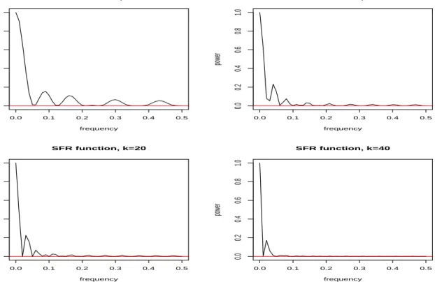
In Figure 1 I plot|R(ω)|2 against frequency for various values of k= 8,16,20,40. Assuming
that k is selected as k = √n these values correspond to the following sample sizes: 16 years of quarterly observations, 64 years of quarterly or 21 years of monthly observations, and over 5 years of daily observations. As expected, we see that the smoother enhances the low frequency component of the original series but for low values of k allows for some power to pass from higher frequencies. It is possible to select the value of kso as to significantly reduce the power at certain frequencies. For example, taking k equal to the cycle period (e.g. 4 for quarterly or 12 for monthly data) we can smooth the original series retaining the low frequency component and erasing most of the cyclical component, if one exists. In Figure 2 I plot |R(ω)|2 against
frequency fork= 4,12 and mark the frequency that corresponds to the period noted before. We can also examine the properties of the residual series us,1 def= xs−xs,1. First note that,
using the factorization of the filter polynomial in equation (25), we have that, fork≤s≤n−k+1:
us,1= [1−ψ(L)]xs=
h
1−k−2Lk−1ψ∗(L−1)
i
xs (27)
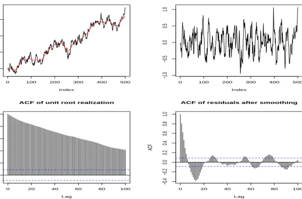
so that the residuals can be thought of as k −1-period ‘quasi-differences’. Note that these residuals contain forward looking information about the series, they are computed using terms after xs. In this sense one can possibly call them ‘predictive residuals’. In Figure 3 I plot the sample realization from a unit root process withηt∼ N(0,0.22),n= 500 andk= [
√
the sample autocorrelation function of the original series and the residual series. The differences in the behavior between the two series are apparent. Moreover, note that after the removal of the smooth component there is a substantial amount of serial correlation that remains in the residual series. However, this autocorrelation can be adequately addressed using a standard autoregressive model to account for the cyclical patterns in the residual autocorrelation function. All the above present an entirely new result that justifies the use of moving averages as optimal smoothers in the context of unit root processes. The implications for the use of moving averages in smoothing and trend extraction of economic and financial time series are evident: the proposed method allows for a precise extraction of the main k components of a stochastic trend using an optimization-based approach, with explicit expressions for the resulting smoothing weights and specific properties attached to the smoothed and residual series.
3.3 Connection with Phillips’ Approximation and Signal Extraction Problems
There are certain similarities and differences between the approach taken in the work of Phillips, say e.g. (2005), the approach of “non-stationary signal extraction”, e.g. Bell (1984), and the current approach. The main similarities between the current approach and Phillips’ approach is that the smoothing of the unit root process is based on asymptotic considerations and that both approaches use versions of the Karhunen-Lo`eve (KL) decomposition. In particular, here I use the asymptotic minimum norm approximation (the sample KL version) and the resulting eigenvector to construct the smoothed seriesxs,1. Phillips motivates his smoother by the use of the KL decomposition to the limit process of the appropriately scaledxtgiven by:
1 √ nx[n·]⇒B(r) def =√2 ∞ X j=1 sin [(j−1/2)πr] (j−1/2)π ξj (28)
forr∈[0,1] and theξj being i.i.d. normal random variablesξj ∼ N(0, σ2). The above theoretical
relationship can be empirically fitted using observations from a realization and can also be used for trend prediction. Letting
n
φj(r)def=√2 sin [(k−1/2)πr]
o∞
j=1denote the system of orthogonal
deterministic functions of time we have the linear regression:
xtdef=xbt,k+ubt,k=
k
X
j=1
bbjφj(t/n) +ubt,k (29)
where k denotes the number of ‘trend coordinates’ that are to be used in reconstructing the series. For k → ∞ and k = o(n) we have that the above regression can reproduce the entire realization. For low values ofkone can extract the underlying trend components. Note that the regression coefficient estimatorsbbj converge to random variables in this context, not constants (see Phillips (2005) and references therein for details).
While in essence both approaches are trying to do the same thing, i.e. smooth the realization of a unit root process, there are also two differences between them. First, the approach of Phillips (2005) is a global approach, as it is based on the application of global least squares to the entire realization for extracting the trend components. The smoothing is a by-product of this global fitting, essentially through the use of the trigonometric basis functions. In contrast, the current approach is a local approach as it is based on the application of local smoothing via the use of moving averages. Of course both approaches can achieve the same degree of smoothing by appropriate choices of the smoothing parameter k. A second difference is that the method in Phillips (2005) does not come out of an optimization framework and does not come with a ‘structural’ interpretation. With ‘structural’ interpretation I simply mean that the approach that is proposed here is related to a well-understood notion of smoothing, that of a moving average. It is obvious that both methods have well-defined interpretations in the context of the unit root assumption. Finally, note that the choice of the smoothing parameter is opposite in the two methods: in the SSA-based method of the previous section more smoothing is performed by allowing k to increase; in Phillips’ method more smoothing is performed by allowing k to decrease.
There are more differences than similarities with other methods that have as their basic idea that of “signal extraction” or the isolation of a particular, well-defined component of the under-lying stochastic process Xt using the realization Xn. An important, theoretical and practical
difference, is that all such methods require the a priori specification of a parametric model for the “signal” and the ”noise” (whose precise definition varies by discipline). Without postulating such a model it is not possible to apply any of the optimal filters that appear in the relevant literature. Such a model comes with along with parameter estimation, estimation uncertainty, the possibility of structural breaks, misspecification, etc. This is not to claim that problems like structural breaks cannot occur within the unit root framework; they do. However, the simplicity of the unit root model, and the proposed smoothing method of this paper, do have a certain sense of robustness to such problems.
To illustrate the differences between smoothing in the signal extraction framework and the current framework consider a simple example: the random walk plus noise model (also known as local level model). Let Yt denote the observable stochastic process and let Xt denote the
unobservable signal, which has a unit root. They are assumed to be related by the following state space model:
Yt = Xt+²t
Xt = Xt−1+ηt
where ²t ∼i.i.d.(0, σ2
²) is the observational noise and where ηt ∼i.i.d.(0, σ2η) is the signal noise,
with ²t independent of ηs for all (t, s). The properties of this model depend on the
“signal-to-noise” ratioq def=σ2η/σ²2: asq→0 the signal is buried in noise and is difficult to recover; asq → ∞
the model collapses to the standard unit root model of equation (18). Accurate MSE extraction of the signal component requires estimation (via the Kalman filter) of the two variance parameters and then fixed point smoothing. Is the method proposed in this paper capable of separating the signal from the noise in this set-up? To examine this let us construct the relevant trajectory matrices and the corresponding autocovariance matrices. Denoting the trajectory matrices in standard fashion as TY,TX and T² and the corresponding matrices of sample autocovariances
asΓbj(k) for j=Y, X, ²we immediately obtain:
TY =TX +T²
b
ΓY(k) =ΓbX(k) +Γb²(k) +ΓbX,²(k) +Γb²,X(k)
(31)
where ΓbX,²(k),Γb²,X(k) are the cross-covariances between the signal and the noise trajectories. Under the assumptions of equation (30), and using standard results, we have that asymptotically
b
Γ²(k) ⇒ σ2²Ik and Γb²,X(k) ⇒ χ, where χ is a stochastic matrix. However, since ΓbX does not
converge unless scaled bynwe end up havingn−1Γb²(k)⇒0k,k,n−1Γb²,X(k)⇒0k,kand therefore:
1 nΓbY(k)≈ 1 nΓbX(k)⇒σ 2 ηwJk,k (32)
exactly as in equation (19). This result has not appeared in the SSA or filtering literature and is of practical significance: using SSA for a unit root process contaminated with noise we can extract the underlying non-stationary signal directly, at least asymptotically. Combining previous results on stationary SSA with the results from the previous sections we can also select
k, the degree of smoothing appropriately: asq →0 thenk→n/2 withn→ ∞; as q→ ∞ then
k=o(n), e.g. k=√n.
For comparison with the SSA approach I reproduce below McElroy’s (2005) matrix-based formulas for Kalman fixed point smoothing for the local level model. Letting ∆ denote the (n×n−1) matrix with -1 on its principal diagonal and 1 in its first lower diagonal andYn def=
[y1, y2, . . . , yn] denote the (1×n) vector of observations we have that the (n×n) matrix of optimal
smoothing coefficients is given by:
Fn(σ2², ση2)≡Fndef=ση−2 ³ ∆∆>σ−²2+Inσ−η2 ´−1 = ³ ∆∆>q+In ´−1 (33) so that the optimal MSE signal estimate is given bycXndef=E[X|Y] =YnFn.
Figure 4 illustrates the above using a sample realization from equation (30) with both ²t
the signal variance, and with k = √n as before. The lower panel of the figure shows the true signal and the two smoothed series, the one based on SSA and the other on the application of fixed point smoothing (with the parameters estimated). It is clear from the figure that the non-parametric SSA smoother performs on par with the parametric fixed point smoother. We further explore the performance of the proposed methodology in the context of signal extraction in the simulation section.
Remark 1. In the signal extraction framework one can accommodate a comparison between the proposed method and the Hodrick-Prescott (1997) HP-filter that is used frequently in trend extraction and smoothing in economics. It can be shown, see for example Schlicht (2005), Dermoune et al. (2007) and earlier references therein, that the HP filter can be derived from a signal extraction model similar to equation (30) but where the signal processXthas two instead
of one unit roots, i.e. (1−B)2X
t=ηt, withB being the backshift operator. The filtered values
can be computed using exactly the same formula as in equation (33) before with∆being defined as (n×n−2) with -2 on its principal diagonal and 1’s on the first upper and lower diagonals. Schlicht (2005) and Dermouneet al. (2007) also proposed methods to consistently estimate σ2
η,
σ2
² andq from the data. The method proposed in this paper can easily be used in the HP model
context and we illustrate this in the empirical applications’ section.
3.4 Trend Prediction
Both the signal extraction approach and Phillips’ (2005) approach can be used to extrapolate the smoothed series and thus make signal/trend predictions. The signal extraction formulas are well known and thus omitted. Phillips (2005) also provides an explicit expression for theh-step ahead predictor for the fittedk trend components, sayxbt+h,k.
Below I give the h-step ahead trend predictor based on the SSA method and the resulting smoothed series. Using known results from SSA about the continuation of reconstructed com-ponents, see Golyandina et al. (2001), the formula the defines the extrapolation coefficients is given by: α= 1 1−ν2 r X j=1 uk,jukj−1 (34)
where ν def= u2k,1+u2k,2+· · ·+u2k,r is the sum of squares of the last element of the eigenvectors
j= 1,2, . . . , r(called the verticality coefficient) and whereujk−1denotes the (k−1×1) vector with
the firstk−1 elements of eigenvectorsj= 1,2, . . . , r. Successful continuation of a reconstructed component, i.e. the smoothed series, requires thatν2 <1.
In the current context we have that r = 1 and u1 has the particularly simple form u1 =
Jk/
√
k. Note that the verticality coefficient becomes ν2 = 1/k which is always less than one
and thus the predictor is well defined. Doing some algebra we finally get that the prediction parameter vectorαsimplifies toα= [1/(k−1),1/(k−1), . . . ,1/(k−1)]>and the the smoothed series h-step ahead prediction is defined recursively as a simple average of its pastk−1 values, that is: b xs+h,1= k−1 1 k−1 X j=1 b xs+h−j,1 (35)
3.5 Selecting the degree of smoothing
A practical problem is how to select the degree of smoothing. Both the current methodology and Phillips’ methodology cannot use an MSE-like criterion for selecting the degree of smoothing since there is no underlying model that defines a signal. Is there any other way in which we can select the degree of smoothing based on an optimization criterion? I propose such a criterion below, applicable both to the current methodology and to Phillips’ methodology, and structure the problem as follows. To maintain the idea of smoothing and trend extraction k should be kept relatively high (low) and an appropriate value should be selected based on a different objective function than the residual error variance, i.e. the MSE. A suitable alternative could be the following. Assume that you would like to fit the “correct trend on average”. You would then expect to obtain about an equal amount of positive and negative residuals: sometimes the actual series would be higher than the smoothed trend and sometimes it would be lower. An objective function that fits this idea is the (absolute value of the) average sign of the residuals from the selected smoothed trend. Minimizing this function we can not only obtain a meaningful “optimal” value ofk but we can also compute appropriate residual error bands.
More formally, for any valuek∈ {kmin, . . . , kmax} define the average sign of the fitted resid-uals4 as: b m(k)def= 1 n n X t=1 sign(ut,1) (36)
Since the sign function can be decomposed as sign(x) = I(x > 0)−I(x < 0), for I(·) being the indicator function, we can also decomposemb(k) as mb(k) =mb+(k)−m−(k), the respective averages of the positive and negative residuals. A plausible ‘optimal’ choice for k is that value that minimizes the absolute value ofmb(k), that is the value that produces, on average, an equal
4I use the notation for the residuals of the proposed method in the paper,u
t,1 but the same can be done with
number of positive and negative residuals, that is mb+(k) ≈ mb−(k). This value, say k∗, would give the trend component of the series that will be an approximately “unbiased” estimate of the series’ main trend component. We have then thatk∗ would be given as solution to the following optimization problem:
k∗ : argmin
k∈{kmin,...,kmax}
|mb(k)| (37)
There is no rule for selecting kmin and kmax but one can follow the suggestions in the end of
section 3.3 after equation (32). For Phillips’ approach kmin can be taken to be 1 but this will
not work for the SSA approach wherekmin≥2.5
If one wants to use predicted trend values, saybxt+h,1 in selectingk∗ then a suitable approach
is historical simulation, which can be done as follows. Split the available realization in two parts ofn0+n1 =nobservations, an estimation and an evaluation sample respectively. Using a rolling
window ofn0 observations computen1−h h-step ahead out-of-sample trend predictions. Then, for each value of k, compute:
b
m1(k)def= (n1−h)−1
nX−h t=n0+1
sign(but+h,1) (38)
whereubt+h,1 def= xt+h−xbt+h,1 and findk∗ from minimizing|mb
1(k)|.
Based on the predictions fromk∗one can form the corresponding residual deviationsub∗t+h,1 def=
xt+h−xbt∗+h,1 and compute their standard deviation, saysk∗. Using the standard deviation one
can construct trend prediction bands [L(τ), U(τ)] given by: [L(τ), U(τ)]def=£xb∗t+h,1−τ·sk∗,bxt∗+h,1+τ·sk∗
¤
(39) for anyτ ∈R+. An interesting empirical question that relates to these prediction bands is their coverage ratio, i.e. the fraction of out-of-sample observations that fall within the bands during the evaluation sample. This ratio is defined as:
CR(τ)def= (n1−h)−1
nX−h t=n0+1
I{L(τ)≤xt+h≤U(τ)} (40)
I further explore this method for selecting k and its properties in the simulation section that follows.
3.6 Cointegration and common stochastic trend extraction
The methodology proposed in the earlier sections of the paper can be extended to handle common stochastic trend extraction in the context of a simple bivariate cointegrating system - systems
5In fact in both approachesk
of larger dimension should, in principle, be handled in a similar fashion but I do not pursue this here. Phillips (2005) has, in the context of his methodology, a much more comprehensive treatment of cointegration in the context of stochastic trend extraction.
Consider a unit root process Zt that is the (unobservable) common stochastic trend
compo-nent of two other non-stationary processesYtandXtthat are related by the following system of
equations:
Yt = αZt+²t
Xt = Zt+ut
Zt = Zt−1+ηt
(41)
with ²t ∼ i.i.d.(0, σ2²), ut ∼i.i.d.(0, σ2u) and ηt ∼i.i.d.(0, ση2) where I assume for simplicity that
²t, us, η` are independent for all (t, s, `).
It is easy to see that Yt and Xt are cointegrated, i.e. a linear combination of them forms a
stationary process, with the scalar parameter α being the cointegrating coefficient. To see this note that:
Yt−αXt = αZt+²t−αZt−αut→
Yt = αXt+ζt
(42)
where ζt def= ²t−αut is a stationary process. The inference problems here are (a) estimation of
theα parameter and (b) extraction of a smoothed version of the common stochastic trendZt.
It should be immediately clear that (b) above can easily be handled by a straightforward application of the signal extraction approach of equations (30) to (32) to theXtprocess. However,
there is potential loss of information in doing this since Zt enters into both Yt and Xt and the two series are connected — not to mention the case where ²t, us, η` are not i.i.d. and dependent
between them. Therefore a more efficient approach would be to use information from both processes in extracting Zt and in what follows I propose an SSA-based way to handle both (a)
and (b) above.
The estimation ofα can be accomplished immediately if we use the properties of the matrix of the autocovariances for each process. Using a similar notation to equations (30) to (32), and the corresponding properties of the series, note that we have:
n−1ΓbY(k)≈α2n−1Γb
Z(k)⇒α2ση2wJk,k
n−1ΓbX(k)≈n−1Γb
Z(k)⇒ση2wJk,k
(43) The above relationships suggest a simple estimator for α based on the empirical (estimated) eigenvalues of the two autocovariance matrices. We have:
Proposition 2. Under the assumptions of equation (41) and the properties of Propo-sition 1 we have that a consistent, SSA-based, estimator of the cointegrating cofficient
α is given by the square root of the ratio of the two leading estimated eigenvalues of
n−1ΓbY(k) and n−1ΓbX(k) as: b αdef= q b λ1,Y/bλ1,X ⇒α (44)
The finite sample properties of the above estimator are briefly examined in the simulation analysis of the next section.
Once an estimator of α is available we can combine information from both Yt and Xt in ex-tracting a smoothed version of the unobserved common stochastic trendZt. This is accomplished
by averaging as before:
Yt+αXt = 2αZt+²t+ut→
Ψt(α)def= (2α)−1(Yt+αXt) = Zt+ξt
(45) where ξt def= (2α)−1(²t+ut). We can now apply SSA to the empirical counterpart of Ψt(α), i.e.
ψt(αb) or combine the individually SSA-smoothedYtand Xt series directly as:
ψs,1(αb)def= (2αb)−1(ys,1+αxb s,1) (46)
The resultingψs,1(αb) series would be the smooth approximation to the common stochastic trend
componentZt and will utilize information from bothYt andXt. If no smoothing is desired then
the common stochastic trend component is directly approximated byψt(αb). The performance of
the above smoother is also briefly examined in the simulation analysis that follows.
4
Simulation Analysis
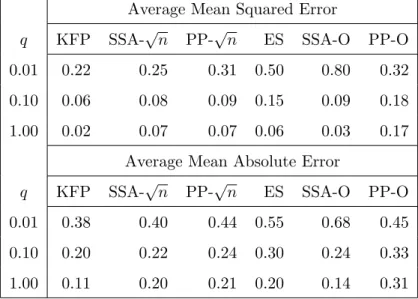
In this section I evaluate the proposed methodology using three simulations. For the first simu-lation I use as the data generating process the local level model of equation (30) with different values for the signal-to-noise ratio q and different assumptions on the distribution of ηt. For a sample size of n = 250 observations I perform signal extraction using: (a) the Kalman fixed point smoother of equation (33); (b) the SSA approach of this paper with fixedkandk∗; (c) the approach of Phillips with fixed k and k∗; and (d) exponential smoothing. For (a) and (d) the relevant parameters are estimated from the data. I perform 500 replications and report average mean-squared and mean-absolute errors for the residuals from the true signal. Specifically, if
b
xt,ij denotes the signal estimate for theith replication for thejth method I compute:
AM SEj def= 5001 500 X i=1 " 1 n n X t=1 (xt,i−xbt,ij)2 # , AM AEj def= 5001 500 X i=1 " 1 n n X t=1 |xt,i−bxt,ij| # (47)
For the same simulations I also report the average value of the selectedk∗using the methodology of the previous section. These results are summarized in Tables 1, 2 and 3.
The results in Table 1 are extremely encouraging. The fixedk=√nfilter is very competitive to the Kalman fixed point filter, which is optimal for the data generating process. For the AMSE on the top panel of the table we can observe that asq increases the performance of the optimal
k∗ filter also becomes very competitive to the Kalman filter, eventually matching it. For the AMAE on the bottom panel of the table we see a similar situation as with the AMSE results. Overall we can say that (a) the fixedkSSA-based filter of this paper can be used reliably for this type of data generating process; and (b) the optimalk∗ SSA-based filter is to be preferred when the signal-to-noise ratio is relatively large. Phillip’s smoother is trailing after the SSA smoother, its performance being slightly worse. The exponential smoother performs well only for q = 1, as expected. Finally, the results in Table 2 summarize the average k∗ that was selected across replications.
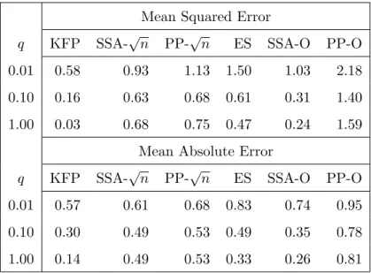
In Table 3 I present a variation of the results in Table 1. Here I take the signal noise to have been generated by a Studentt(2) distribution scaled by a factor ση. This distribution does not
have finite second moments so the meaning of q is not the same as before. Nevertheless it is instructive to look at the performance of the various filters. We can see that the performance of almost all filters deviates more substantially than before from the performance of the Kalman fixed point filter and their differences do not significantly diminish as q increases (this was expected since for any value ofq the signal has infinite variance.) It is only the optimalk∗ SSA-based filter that can come close to the Kalman fixed point filter and its performance improves asq increases.
For the second simulation I examine the out-of-sample prediction approach for selecting the degree of smoothing given in equations (38) to (40). I generate 500 replications from a unit root model of size n = 250 observations. I then use a rolling window of n0 = 200 observations and an evaluation period ofn1 = 50 observations to construct trend prediction bands as in equation
(39) and to examine the coverage ratio of equation (40). I takeτ = 1, i.e. to consider prediction bands one standard deviation away from the trend. The results in Table 4 below present: the average coverage ratio (ACR), its standard deviation (SD), the median coverage ratio (Q0.50), the 10% and 90% quantiles of the coverage ratio (Q0.10andQ0.90), and the average selected value
of k∗.
The results between the SSA approach and Phillip’s approach are similar. The average coverage ratio is about 66% and its distribution is symmetric (the median coverage ratios are practically the same as the mean coverage ratios). This is quite suggestive, given the underlying
normality of ηt, since the coverage probability of a standard normal distribution between ±1 (standard deviations) is about 68%. In addition we can observe that, on average across repli-cations, the standard deviation of the coverage ratio is proportional to the difference between the two quantiles, i.e. (Q0.90−Q0.10)/SD≈1.22 (1.17 for SSA and 1.28 for Phillips); the
corre-sponding ratio in a standard normal distribution is 1.65. These descriptive statistics, which are based only on 50 observations, are very supporting the proposed methodology for selecting the degree of smoothing in an out-of-sample context: they indicate that the trend selected in this way is approximately “unbiased”.
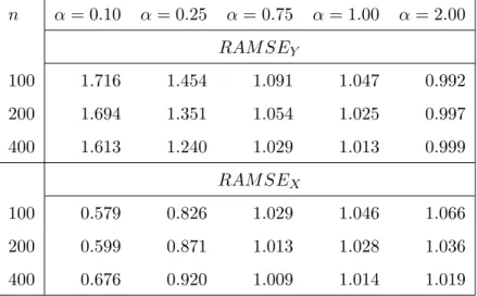
I conclude this section with results from a third simulation, about the finite sample properties of the estimator of the cointegrating coefficient given by Proposition 2 in equation (44) and the properties of the smootherψs,1(αb) in equation (46). I use the system in equation (41) as the data
generating process with different values for the parameters and the sample size. I consider three sample sizesn={100,200,400}and five values ofα={0.10,0.25,0.75,1.00,2.00}. I perform 500 replications, as before, and I compute (a) the average mean absolute deviation of the estimates from their true parameter value and (b) the relative average mean-squared error between the actual common stochastic trend and the corresponding smoother of equation (46). In both cases I take k=√n. Specifically, for the average mean absolute deviation I compute:
AM ADdef= 1 500 500 X i=1 |αbi−α| (48)
The results given in Table 5 indicate that the proposed estimator does a reasonably good job in estimating the true cointegrating parameter and is indeed consistent. It is possible that its performance in small samples is better in an intermediate range of values forα: for n= 100 the largest AM AD is found for the two extremes, i.e. for α = 0.10 and α = 2.00. This disappears for the larger samples.
For the relative average mean-squared error I do the following. In each replication run I compute the smoother of equation (46) as well as the smoothers based onXtalone and on Yt/αb
alone, that can also approximateZt. For each of the smoothers, sayzbt,1, I compute:
AM SE(zbt,1)def= 5001 500 X i=1 " 1 n n X t=1 (Zt−zbt,1)2 # (49) and then report the relative average mean-squared errors as:
RAM SEY def= AM SE(yt,1/αb)
AM SE(ψt,1(αb))
, and RAM SEX def= AM SE(xt,1)
AM SE(ψt,1(αb))
(50) For the results in Table 6 I use the following parameter combination6: σ2
² =σ2u= 0.22,σ2η = 0.12
and the three noise series were drawn from three independent normal distributions. Two results about the performance ofψt,1(αb) are immediately evident:
• ifαtakes small values, hereα= 0.10 andα= 0.25, and we are close to the no cointegration case then using ψt,1(αb) will improve the results compared to using yt,1/αb alone but not
compared to usingxt,1 alone — this is of course expected since in that case its essentially Xt that contains the useful information aboutZt.
• if, on the other hand, α takes larger values then using ψt,1(αb) is better than using either
of the individual smoothers.
All in all the results in Tables 5 and 6 are supportive of the proposed methodology for bivariate cointegrated systems, both for estimation of the cointegrating coefficient and for extracting a smoothed version of the common stochastic trend component.
5
Empirical Illustrations
In this section I present two empirical illustrations of the proposed methodology. First I compare the SSA-based filter of this paper with the Hodrick-Prescott (HP) filter for the series of quarterly observations of the U.S. real GDP (series GDPC96 from the Federal Reserve Bank of St. Louis Database, in billions of chained 2000 dollars). The series has n = 244 quarterly observations from 1947:Q1 to 2007:Q4. Then I use the SSA-based filter for smoothing and trend extraction for the weekly prices of Brent crude Oil and of the Euro/US Dollar exchange rate.7 The series
have n= 477 weekly observarions from 01/04/1999 to 02/19/2008.
5.1 U.S. Real GDP
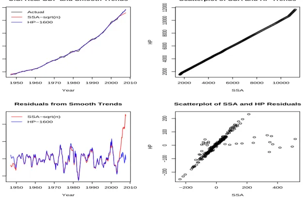
The HP filter has been used widely in smoothing trending economic time series and the original 1997 paper was followed by a large literature on optimal filtering. Here we show that the SSA-based filter of this paper performs on par with the HP filter, either when a naive value is used for the smoothing parameter q or when the value of the smoothing parameter is optimized. Consider first the case where q = 1600, the value suggested by Hodrick and Prescott in their 1997 paper for quarterly data, and compare it with the SSA-based filter withkfixed tok=√n. Figure 5 contains the results. There are several things to notice: first, see that both filters
7These series are used in the EurOil Index project found at http://econ.uop.gr/∼thomakos/EurOil Index.html
achieve practically the same degree of smoothing over the entire length of the series and produce practically identical residuals, with the exception of the end of the series. This is due to the construction of the two filters: in the SSA case the last value of the smoothed trend is an unweighted backward moving average, see equation (22). This can be seen as a shortcoming of the SSA-based filter which brings us to a question: are the two filters, as applied, comparable? The answer is clearly no!
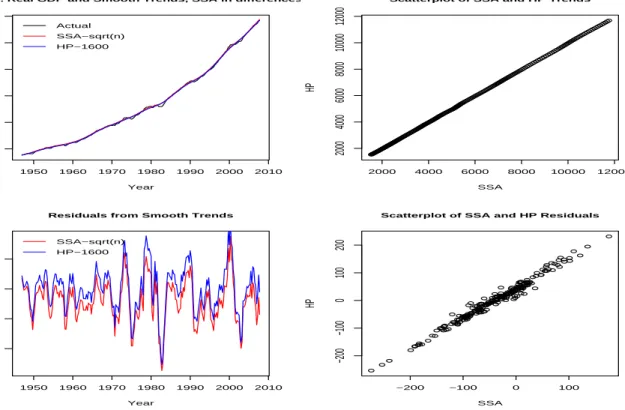
As noted in Remark 1 at the end of section 3.3, the underlying stochastic model on which the HP filter is based is for a time series with two not one unit root. Therefore the results of Figure 5 are OK but are not directly comparable. To make a meaningful comparison we need to apply the SSA filter in the first differences of the GDP series and then cumulate the extracted signal. The results from this approach are presented in Figure 6.
We can now make a meaningful comparison between the two filters and we can see that they now match everywhere, both in the smooth trends and the corresponding residuals; see the differences in the scatterplots between Figure 5 and Figure 6. We therefore see that the proposed SSA-based filter achieves the same degree of smoothness as the standard HP filter, after taking into account the stochastic model under which the HP filter operates.
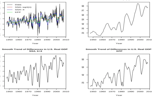
An interesting byproduct of this approach, of applying the SSA filter in the first differences of the GDP series, is the extracted smooth trend. Figure 7 has this trend for bothk=√nand for
k= 4, the latter corresponding to the quarterly frequency of the data - see the squared frequency response fork= 4 in Figure 2. We also present for comparison the smooth trend obtained from applying Kalman fixed point smoothing based on the local level model of equation (30) - the estimated signal-to-noise ratio is qb= 0.068 which makes signal extraction in first differences a more interesting exercise than in levels. Both short and long-term cycles in U.S. output are evident in the three panels of the figure that show the smooth trends. Note the similarity of the SSA-based smooth trend fork=√nand the KFP-based smooth trend - remember that the close performance of these two filtering methods in the context of a similar signal-to-noise ratio was seen in the simulations of the previous section.
In concluding this section I note that all the above analysis was repeated with both kand q
(in HP filter) selected in an optimal fashion but the results were qualitatively similar to the ones already presented and are available on request.
5.2 Oil Prices and the Euro/US Dollar Exchange Rate
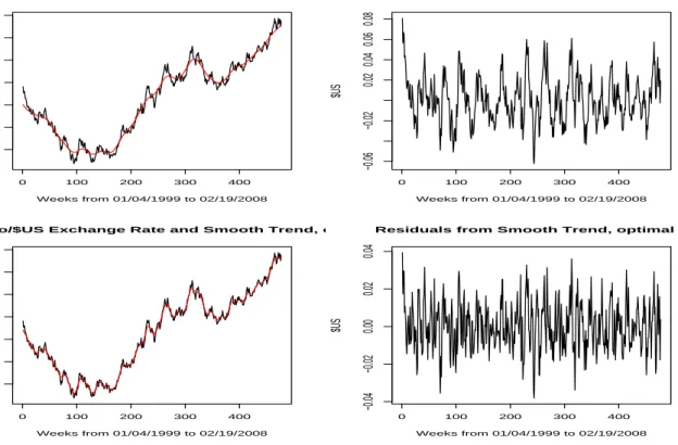
The two financial time series analyzed in this section are different in nature from the U.S. Real GDP series of the previous section. Unlike the GDP series which was quite smooth and a model with two unit roots was more appropriate, the Oil and Euro/US Dollar series exhibit characteristics consistent with one unit root. In this section I present some graphical results from SSA-based smoothing of the two series and also for the construction of prediction error bands for the extracted trends using the methodology at the end of section 3.5.
Figures 8 and 9 contain the results from smoothing the weekly Oil series. Two values for k
are used the fixed valuek=√n= 21 and the optimal valuek∗ = 9. The data with the smooth trends and the corresponding residual series are in Figure 8 while the autocorrelation functions of the residuals are given in Figure 9. Note the similarity between the results in these two figures and the results from a sample realization from a unit root process in Figure 3. In particular note that there is significant residual autocorrelation that exhibits a cyclical pattern. Figures 10 and 11 contain the related results from smoothing the Euro/US Dollar exchange rate series. The optimal value of k in this case wask∗ = 8. The underlying patterns are very similar to that of the Oil series, i.e. are consistent with an underlying unit root process. Whether the cyclicality of the residuals in both series can be (partly) attributed to market conditions or its an artifact of the unit root behavior is of course an open question.
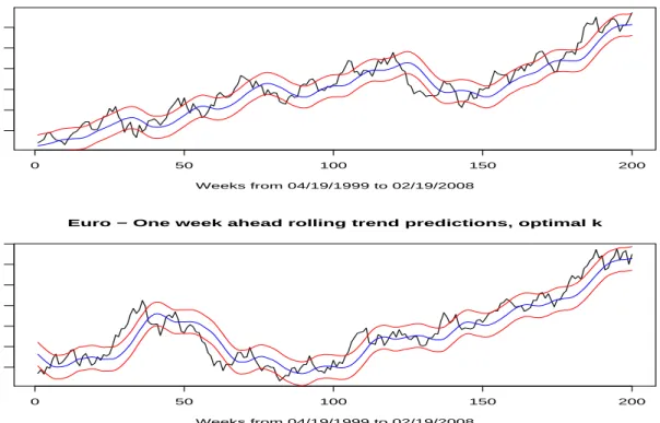
In Figure 12 I present the results from a rolling, one week ahead, out-of-sample trend pre-diction with corresponding one (τ = 1) standard deviation bands. I use a rolling window of
n0 = 277 weeks and an evaluation window of n1 = 200 weeks in the figure. The sk∗’s, the
pre-diction error standard deviations are $5.32 and $0.03, over the 200 weeks evaluation period. The coverage ratio CR(1) of equation (40) was equal to 65% for the Oil and 69% for the Euro/US Dollar series, a proportion quite consistent with the simulation results presented in Table 4. It is interesting to note that for both series their last actual values exceed the predicted trend values; Oil, in particular, is at the upper prediction band. Both series have (as of 02/27/2008) exceeded their trend values.
Finally, I use the methodology of section 3.6 to examine the possibility of extracting a smooth, common stochastic trend component between the two series. After standardizing the data, to express them in a comparable numerical scale, I apply the smoother of equation (46) and present the result in Figure 13. The averaging operation can clearly be seen in the figure as the smooth trend component runs between the two series. It captures quite well the common evolution of these two assets that have moved closely together over time.