NPCirc: An R package for nonparametric circular methods

(1)

October 2014, Volume 61, Issue 9. http://www.jstatsoft.org/

NPCirc

: An

R

Package for Nonparametric Circular

Methods

Mar´ıa Oliveira University of Santiago de Compostela Rosa M. Crujeiras University of Santiago de Compostela Alberto Rodr´ıguez-Casal University of Santiago de Compostela Abstract

Nonparametric density and regression estimation methods for circular data are

in-cluded in theRpackageNPCirc. Specifically, a circular kernel density estimation

proce-dure is provided, jointly with different alternatives for choosing the smoothing parameter. In the regression setting, nonparametric estimation for circular-linear, circular-circular and linear-circular data is also possible via the adaptation of the classical Nadaraya-Watson and local linear estimators. In order to assess the significance of the features observed in the smooth curves, both for density and regression with a circular covariate and a linear response, a SiZer technique is developed for circular data, namely CircSiZer. Some data examples are also included in the package, jointly with a routine that allows generating mixtures of different circular distributions.

Keywords: circular data, CircSiZer, nonparametric methods, mixtures,Rpackage.

1. Introduction

Statistical methods for circular data analysis have turned out to be the appropriate tools in many applied fields, such as biology (Batschelet 1981), ecology (Jammalamadaka and Lund 2006), meteorology (Bowers, Morton, and Mould 2000), sociology (Brunsdon and Corcoran 2005), medicine (Mooney, Helms, and Jollife 2003) or biomechanics (Mann, Gupta, Race, Miller, and Cleary 2003), among others. From a methodological perspective, most of these applied papers make use of circular descriptive techniques, providing graphical displays of the data such as rose diagrams, and in some cases, classical parametric inferential tools are considered, with the von Mises distribution being a cornerstone in this approach.

Modeling circular data distributions by means of parametric families has been covered in most of the papers in the statistical literature. Comprehensive reviews such asMardia(1972),

(2)

Fisher (1993), Jammalamadaka and SenGupta (2001) and Mardia and Jupp (2000) present parametric models such as the aforementioned von Mises, the cardiod, or the wrapped-normal distributions, among others, jointly with testing procedures for assessing uniformity, such as Rayleigh’s, Kuiper’s, Rao’s spacing or Watson’s tests. Although being widely used, the von Mises model is not flexible enough to capture the underlying structure of multimodal, highly peaked or skewed distributions. Some new parametric models for handling these fea-tures have been presented byAbe and Pewsey (2011), who introduced circular models with two diametrically opposed modes, or Jones and Pewsey (2012), who proposed the inverse Batschelet distribution, accounting for skewness and high kurtosis. The consideration of mixtures of parametric models may offer a route to capture complex structures, but at the cost of increasing the number of parameters characterizing the distribution. In this setting parametric estimation can be done by maximum likelihood arguments using the expectation-maximization (EM) framework as inBanerjee, Dhillon, Ghosh, and Sra(2005), and model fit can be approached by means of an information criterion. Nevertheless, the specification of an appropriate parametric family may not be an easy task.

Nonparametric estimation methods have turned up as an alternative approach, both infer-entially and as a descriptive tool. Specifically, a kernel density estimation procedure was proposed byHall, Watson, and Cabrera(1987), for the general case of spherical data, follow-ing the ideas of the classical kernel density estimator for linear data (Parzen 1962;Rosenblatt 1956). Although asymptotic properties of this estimator were further studied by Bai, Rao, and Zhao (1988) and Klemel¨a (2000), these latter works do not provide a solution for the most critical issue from a practical point of view: smoothing parameter selection. The use of cross-validation smoothing parameters is suggested byHall et al. (1987), in the spherical context, and for the particular case of circular data, Taylor (2008) derived a rule of thumb for smoothing parameter selection in circular kernel density estimation. Despite being a simple procedure, the performance of this rule is extremely poor in some distribution set-tings involving multimodality, peakedness or skewness, as shown byOliveira, Crujeiras, and Rodr´ıguez-Casal(2012). Marzio, Panzera, and Taylor(2011) introduced a bootstrap method with the same purpose, but with unsatisfactory results for small data samples. Recently,

Oliveira et al.(2012) devised a new procedure for selecting the smoothing parameter in cir-cular kernel density estimation that performs well in distributional scenarios beyond the von Mises case, and presents better or at least competitive results compared with the previously proposed selectors.

Regression estimation involving circular variables, as a response or as a covariate, is indeed an interesting problem. In the available literature, most efforts have been focused on the development of parametric models. For instance, Presnell, Morrison, and Littel (1998) and the references therein dealt with a circular response and linear covariates; SenGupta and Ugwuowo (2006) proposed some asymmetric models accounting for the circular nature of the covariate and Downs and Mardia (2002) and Kato, Shimizu, and Shieh (2008), among others, addressed the regression with circular response and covariates. Regression estimation avoiding the assumption of a specific parametric shape for the regression curve was studied by Marzio, Panzera, and Taylor (2009) who extended the least squares local polynomial to the case ofd-dimensional circular predictors and real-valued responses;Qin, Zhang, and Yan

(2011a,b) extended nonparametric models to the case when there is one circular predictor and one or more linear predictors and the response is real-valued, and more recently Marzio, Panzera, and Taylor (2012) proposed a nonparametric estimator for the regression function

(3)

when the response is circular and the covariate is circular or linear. In the regression setting, the smoothing parameter can be chosen by cross-validation methods.

Both for density and regression estimation, the smoothing parameter controls the global ap-pearance of the estimator and its dependence on the sample, and it is well-known that an unsuitable choice of this value may provide a misleading estimate of the density or the re-gression curve. Hence, the assessment of the statistical significance of the observed features through the smoothed curve may be seriously compromised if an undersmoothed or an over-smoothed estimator is produced. An alternative to circumvent the choice of the smoothing parameter, and still be able to assess global structure features in the curve, is given by the SiZer (significative zero crossing of the derivative) method developed byChaudhuri and Mar-ron (1999) for the analysis of linear data. The idea behind this technique is to determine the regions of significant gradients (zero crossing of the derivative) over a range of smooth-ing values. The SiZer ideas have been adapted to the circular settsmooth-ing, both for density and circular-linear regression, as proposed by Oliveira, Crujeiras, and Rodr´ıguez-Casal (2014a), by means of the CircSiZer map.

PackageNPCirc (Oliveira, Crujeiras, and Rodr´ıguez-Casal 2014b) described in this paper is intended to provide R (R Core Team 2014) users with a comprehensive set of functions for nonparametric density and regression analysis with circular data. There are other packages for working with circular data, already available inRbut, at the best of our knowledge, none of them is devoted to nonparametric methods. Some useful references to work in R with circular data are:

CircStats(Lund and Agostinelli 2012): This package provides methods for the descrip-tive and inferential statistical analysis of directional data. It is based on the book “Topics in Circular Statistics” by Jammalamadaka and SenGupta (2001). Functions

implemented in this package are also available in thecircular package.

circular (Lund and Agostinelli 2013): An extension of the CircStats package, circular provides functions for the statistical analysis (descriptive statistics, circular models, tests), graphical representation and some circular datasets.

CircNNTSR (Fern´andez-Dur´an and Gregorio-Dom´ınguez 2013): Functions for con-structing circular distributions based on nonnegative trigonometric sums, estimating parameters and plotting the constructed densities, are included herein.

isocir (Barrag´an and Fern´andez 2014): This package provides a set of routines for analyzing angular data subjected to order constraints on a unit circle.

movMF (Hornik and Gr¨un 2014): Focused on mixtures of von Mises distributions, this package allows to draw random samples from these models and to proceed with parameter estimation, by using an EM algorithm.

A specific function for kernel density estimation for circular data, and three functions for smoothing parameter selection, have been already included in package circular. These selec-tors are the cross-validation rules proposed byHallet al.(1987) and the rule of thumb intro-duced byTaylor(2008). Apart from this, there is no other function for nonparametric regres-sion estimation and smoothing parameter selection available. From the parametric perspec-tive, packagescircular,CircStats and movMFallow to compute the density function and do

(4)

random generation of mixtures of von Mises distributions but, it is not possible to do the same with mixtures of different circular distributions. Hence, the functions inNPCircwill comple-ment other implecomple-mentations of circular data analysis in three ways. Firstly, in this package, the circular kernel density estimator with an up-to-date collection of smoothing parameter selection procedures are included; Nadaraya-Watson and local linear estimators for circular-linear, linear-circular and circular-circular data, with the corresponding least squares cross-validations rule for smoothing choice, have been also implemented. Secondly, CircSiZer maps for density and regression for a circular covariate and a linear response can be also obtained. Finally,NPCirccontains functions for generating data and obtaining densities of a variety of circular models, and mixtures of them. Specifically, the collection of circular models presented inOliveira et al. (2012), can be directly generated. The package is available from the Com-prehensiveRArchive Network (CRAN) athttp://CRAN.R-project.org/package=NPCirc. The structure of this paper is as follows. Section2provides a brief overview on kernel density estimation for circular data, and regression estimation involving circular variables, revising different smoothing parameter selection procedures in both settings. The CircSiZer map is also briefly described here. In Section 3, usage of functions and datasets in the package are described and illustrated. Finally, some remarks are given in Section 4, discussing further extensions of the package.

2. Nonparametric circular methods

As mentioned in Section1, classical parametric circular models may not be flexible enough to capture complex data distributions, and it is in this scenario where nonparametric methods play an important role. Nevertheless, before presenting the circular kernel density estimator and, in order to understand its construction, the von Mises distribution and mixtures of circular distributions are introduced.

The von Mises distribution,vM(µ, κ) (von Mises 1918) is a symmetric unimodal distribution characterized by a mean direction µ ∈ [0,2π), and a concentration parameter κ ≥ 0, with probability density function

f(θ;µ, κ) = 1 2πI0(κ)

exp{κcos(θ−µ)}, 0≤θ <2π, (1) where Ir(κ) denotes the modified Bessel function of order r (see Jammalamadaka and Sen-Gupta 2001, Section 2.2.4). The mean direction coincides with the mode, whereas the pa-rameter κ measures the concentration around the mean direction µ in such a way that, as κ increases, the density peaks higher around µ. As commented before, most of the classical parametric models are unimodal and symmetric (e.g., von Mises, cardioid, wrapped normal, wrapped Cauchy, . . . ), except for the wrapped skew-normal (Pewsey 2000) which is asym-metric.

More flexible models, allowing for multimodality and/or asymmetry, can be obtained by mixing a finite numberM of circular distributionsfm,m= 1, . . . , M, with density

f(θ) = M X m=1 pmfm(θ), with M X m=1 pm= 1, (2)

where pm >0 is the proportion of the density fm in the mixture. Although mixture models

(5)

the cost of including a possibly large number of parameters, usually estimated by maximum likelihood arguments. In addition, the selection of the number of density components in the mixture is another problem, that may be approached by considering some kind of information criterion such as the Akaike information criterion (AIC).

Next, the circular kernel density estimator will be briefly described, jointly with an overview of the smoothing parameter selection methods that are included in theNPCircpackage.

2.1. Circular kernel density estimation

Given a random sample of angles Θ1,Θ2, . . . ,Θn∈[0,2π) from some unknown circular density

f, the circular kernel density estimator off is defined as: ˆ f(θ;ν) = 1 n n X i=1 Kν(θ−Θi), 0≤θ <2π,

whereKν is a circular kernel function with concentration ν > 0 (Marzio et al. 2009), being

the smoothness of the estimated curve controlled by this parameter. As a circular kernel, the von Mises distributionvM(0, ν) (see Equation1) can be considered. With this specific kernel, the density estimator is given by:

ˆ f(θ;ν) = 1 2nπI0(ν) n X i=1 exp{νcos(θ−Θi)}, 0≤θ <2π. (3)

Hence, the estimator can be interpreted as a mixture of n random variables with von Mises distribution, centered in the sample points Θi and with common concentration parameter ν.

A critical issue is the choice of the smoothing parameterν for Equation 3, with large values leading to highly variable (undersmoothed) estimators and small values showing an opposite behavior (oversmoothed curve).

The smoothing parameter is usually selected in order to minimize some error criterion, such as the mean integrated squared error (MISE, MISE(ν) =E(R

( ˆf−f)2_{)). The closed expression} for the asymptotic MISE (AMISE) of the circular kernel density estimator has been derived byMarzioet al. (2009). When ν → ∞and √νn−1→0, the AMISE(ν) is given by:

AMISE(ν) = ( 1 16 1−I2(ν) I0(ν) 2Z 2π 0 f00(θ)2 dθ+ I0(2ν) 2nπ(I0(ν))2 ) , (4)

where f00 denotes the second-order derivative of the target density to be estimated, which measures the curvature off.

The proposal presented byTaylor (2008) for selecting the smoothing parameter is based on the assumption that the data follow a von Mises distribution with concentration parameter κ. In this case, the AMISE expression simplifies and the value of the optimal smoothing parameter, that minimizes AMISE, can be estimated by:

ˆ νRT = " 3nˆκ2I2(2ˆκ) 4π1/2_I 0(ˆκ)2 #2/5 , (5)

where ˆκ is obtained by maximum likelihood estimation. This selector performs satisfactorily in fitting unimodal symmetric distributions, without highly peaked modes but its behavior can

(6)

be dramatically misleading in the presence of antipodal modes and/or skewed distributions, as shown by Oliveira et al. (2012). The poor performance is sometimes due to the non-robust estimation by maximum likelihood of the concentration parameterκ, so a modification of Equation 5 described in Oliveira, Crujeiras, and Rodr´ıguez-Casal (2013) consists of the following procedure:

Step 1. Selectα∈(0,1) and find the shortest arc containing α·100% of the sample data. Step 2. Obtain the estimated ˆκ in such way that R

f(θ, µarc,ˆκ)dθ = α where µarc is the

midpoint of the arc computed in Step 1. The integral is computed over the arc selected in Step1.

Also based on the AMISE minimization, an alternative route to get a smoothing parameter value would be to plug-in as reference density a more flexible distribution, instead of the von Mises model taken by Taylor (2008). For that purpose, a mixture of M von Mises distributions, vM(µi, κi) with proportionspm>0, m= 1, . . . , M can be considered:

g(θ) = M X m=1 pm exp{κmcos(θ−µm)} 2πI0(κm) , with M X m=1 pm = 1. (6)

In that case, the proposed plug-in smoothing parameter selector, ˆνP I, is obtained as follows

(seeOliveira et al. 2012, for further details):

Step 1. Based on the sample information, select the number of mixture components M for the reference distribution.

Step 2. Estimate the parameters in the von Mises mixture (Equation 6), (µbm,bκm,pbm), for

m = 1, . . . , M and compute the integral R

(ˆg00(θ))2dθ. plug-in this quantity in the AMISE expression (Equation4) to getAMISE(ν).d

Step 3. Minimize AMISE(ν) and obtain ˆd ν_{P I}.

In Step1, the selection of the number of mixture components in the reference distribution can be done by AIC, considering different numbers of mixture components, namelyM. Maximum likelihood estimation via the EM algorithm (Banerjeeet al.2005) is used in Step2. In Step3, an optimization method can be implemented, in order to minimize the AMISE.d

Cross-validation rules, as the ones proposed by Hall et al. (1987), are also an alternative for smoothing parameter selection in circular data problems. The likelihood cross-validation smoothing parameter ˆνLCV is obtained by maximizing:

LCV(ν) = n Y i=1 ˆ f−i(Θi;ν), (7)

where ˆf−i denotes the circular kernel density estimator (Equation 3) leaving out the ith

observation. The least squares cross-validation smoothing parameter is obtained as the value ˆ νLSCV that minimizes: LSCV(ν) = Z 2π 0 ˆ f2(θ;ν)dθ− 2 n n X i=1 ˆ f−i(Θi;ν). (8)

(7)

Oliveiraet al. (2012) showed that ˆνLCV provides reasonable results except for highly peaked distributions and, in general, it is more stable that ˆνLSCV.

Finally, Marzio et al. (2011) introduced a bootstrap method for choosing the smoothing parameter. The idea is to take the value that minimizes the bootstrap version of MISE, which has a closed expression when the von Mises kernel is used. The main drawback of this method is that the function to minimize has a global minimum atν = 0 leading to a uniform circular estimate, regardless of the true underlying model. In practice, this will lead to a search for a local minimum, which may pose a problem especially for small samples.

2.2. Circular kernel regression estimation

Kernel regression estimation with circular response and/or covariate are revised in this section. Nonparametric regression for a circular covariate and a linear response

Let{(Θi, Yi), i= 1, . . . , n} denote a random sample from (Θ, Y) a circular and a linear

ran-dom variable, respectively. The relation between these variables may be explained by a regression model such as

Yi =f(Θi) +εi, i= 1, . . . , n, (9)

where f denotes now the regression function and εi are real-valued random variables with

zero mean and varianceσ2 and independent of the Θis. The local circular-linear regression

estimates forf(θ) andf0(θ) are given by ˆf(θ;ν) = ˆaand ˆf0(θ;ν) = ˆb, where

(ˆa,ˆb) = arg min (a,b) n X i=1 Kν(θ−Θi) [Yi−(a+bsin(Θi−θ))]2 (10)

(see Marzio et al. 2009, for further details). As for density estimation, in Equation 10, ν >0 is the smoothing parameter andKν is a circular kernel function with concentrationν.

Usually, a von Mises kernel with concentration parameter ν is considered. If the regression function is locally approximated by a constant instead of using a trigonometric polynomial, the Nadaraya-Watson estimator for circular-linear data is obtained:

ˆ fCNW(θ;ν) = Pn i=1YiKν(θ−Θi) Pn i=1Kν(θ−Θi) . (11)

For both Equations10 and11, the smoothing parameterν controls the degree of smoothing. Large values of ν lead to undersmoothed estimations of the regression curve, tending to an interpolation of the data. On the other hand, small values ofν result in a global averaging, oversmoothing the local features in the data. A simple and widely used procedure for smooth-ing parameter selection in the regression settsmooth-ing is least squares cross-validation, choossmooth-ingν as the value minimizing:

CV(ν) = 1 n n X i=1 h Yi−f−ˆ i(Θi) i2 , (12)

where ˆf−i is the leave-one-out estimator for the regression function, fori= 1, . . . , n. This will

be the method implemented in NPCirc for selecting the smoothing parameter in regression fitting, both for local linear and Nadaraya-Watson estimators.

(8)

Nonparametric regression for a circular response

Let{(∆i,Φi), i= 1, . . . , n}denote a random sample from (∆,Φ), where Φ is a circular random

variable and ∆ will denote a linear or circular random variable. FollowingMarzioet al.(2012), the relation between these variables may be explained by a regression model such as

Φi = [f(∆i) +εi] (mod2π), i= 1, . . . , n,

where the random anglesεi have zero mean direction, finite concentration, and are

indepen-dent of the ∆is.

A nonparametric estimator of the regression functionf at a point δ (which may be real or circular) can be written as,

ˆ

f(δ) = atan2 [ˆg1(δ),ˆg2(δ)],

where the function atan2 [y, x] returns the angle between the x-axis and the vector from the origin to (x, y) and ˆ g1(δ) = 1 n n X i=1 sin(Φi)W(∆i−δ) and ˆg2(δ) = 1 n n X i=1 cos(Φi)W(∆i−δ)

withW being a local weight.

FollowingMarzioet al.(2012), both for a circular or a linear covariate, kernel weights and local linear weights can be considered yielding the Nadaraya-Watson and local linear estimators, respectively. For the case of a circular covariate, the kernel weights are given by taking a circular kernel as weight function and the local linear weights are given by

W(∆i−δ) = n−1Kν(∆i−δ)    n X j=1 Kν(∆j−δ) sin2(∆j−δ) −sin(∆i−δ) n X j=1 Kν(∆j−δ) sin(∆j −δ)    ,

whereKν denotes a circular kernel andν is the smoothing parameter. For the case of a linear

covariate, the kernel weights are given by taking a linear kernel as weight function and the local linear weights are given by

W(∆i−δ) =n−1Kh(∆i−δ)    n X j=1 Kh(∆j−δ)(∆j−δ)2−(∆i−δ) n X j=1 Kh(∆j−δ)(∆j−δ)    ,

where Kh denotes a linear kernel and h is the smoothing parameter. By default, kernels

inNPCirc are von Mises distributions vM(0, ν) for the circular case and N(0, h2) for linear variables.

In both cases, circular or linear covariate, a smoothing parameter (ν or h) must be chosen which may be selected by minimizing one of the following cross-validation functions:

CV(τ) =− n X i=1 cosΦi−f−ˆ i(∆i) , (13)

(9)

CV(τ) = 1 n n X i=1 d2Φi,f−ˆ i(∆i) , (14)

whereτ denotes the smoothing parameter (νorhdepending on the case) anddΦi,f−ˆ i(∆i)

= min(|Φi−f−ˆ i(∆i)|,2π− |Φi−f−ˆ i(∆i)|). By default, the first option will be the method

im-plemented in NPCircfor selecting the smoothing parameter.

2.3. CircSiZer map

From a practical perspective, the concerns about the requirement of an appropriate smooth-ing value for constructsmooth-ing a density or regression estimator may discourage the use of the aforementioned kernel techniques. Indeed, exploring the estimators at different smoothing levels, by trying a reasonable range between oversmoothing and undersmoothing, will pro-vide a thorough perception of the data structure. This idea may be seen as directly feasible by constructing such estimators, but significance of the observed features in the smoothed curve, like peaks and valleys, must be statistically assessed. As proposed by Chaudhuri and Marron (1999), this can be done by studying the zero crossings of the derivative, providing the SiZer map for linear data, and this procedure has been adapted to the circular framework by Oliveira et al. (2014a), via the CircSiZer map included in NPCirc, both for density and circular-linear regression.

In order to assess the statistical significance of features such as peaks and valleys, CircSiZer seeks confidence intervals for the scale-space version f0(θ;ν) ≡ E( ˆf0(θ;ν)), where f is the density or the regression function. A possible way to get such intervals is by means of the “bootstrap t” approach, as detailed in Oliveira et al. (2014a). The output of this procedure is a graphical display, the CircSiZer map, which reflects the statistical significance of f0(θ, ν) with θ∈[0,2π) and ν varying along a range of values. The CircSiZer map is a circular color plot where the performance of the estimated curve for each given value of the smoothing parameter ν is represented by a color ring, in such way that the different colors will allow to identify peaks and valleys. The construction is as follow: for each pair (θ, ν), the curve at a smoothing level ν is significantly increasing (decreasing) if the confidence interval is above (below) 0, so that the corresponding map location is colored blue (red). If the confidence interval contains 0, the curve at the smoothing level ν and at the angle θ does not present a statistically significant slope and it is colored in purple. Regions where there are not enough data to make statements about significance are gray colored. Gray locations are determined according to the estimated effective sample size (see Oliveira et al. 2014a, for details in its calculus). The appearance of the CircSiZer map will be clear in the examples presented in the next section.

3. NPCirc

package

In this section, a detailed description ofNPCirc’s capabilities is provided. The complete list of functions and datasets available inNPCirc, with a brief explanation of each of them, can be seen in Table 1. First, some comments will be made about the datasets included in the package. Functions related to mixture circular models generation and circular kernel density estimation will be described later. Finally, usage of functions for linear, circular-circular and linear-circular-circular regression will be commented. Both for density and circular-circular-linear

(10)

Dataset Description

cross.beds1 Cross-beds azimuths (I)

cross.beds2 Cross-beds (II)

cycle.changes Cycle changes

dragonfly Orientation of dragonflies

periwinkles Snail movements data

speed.wind, speed.wind2 Wind speed and wind direction data

temp.wind Temperature and wind direction data

wind Wind direction data

Function Description

circsizer.density CircSiZer for density

circsizer.regression CircSiZer for regression

circsizer.map Plot a CircSiZer map

dwsn Density function of a wrapped skew-normal distribution

rwsn Random generation from a wrapped skew-normal distribution

dcircmix Density function of mixtures of circular distributions

rcircmix Random generation from mixtures of circular

distributions

kern.den.circ Nonparametric circular kernel density estimation

kern.reg.circ.lin Nonparametric circular-linear regression

kern.reg.circ.circ Nonparametric circular-circular regression

kern.reg.lin.circ Nonparametric linear-circular regression

bw.CV Cross-validation for density estimation

bw.boot Bootstrap method

bw.pi Plug-in rule

bw.rt Rule of thumb

bw.reg.circ.lin Cross-validation for circular-linear regression

bw.reg.circ.circ Cross-validation for circular-circular regression

bw.reg.lin.circ Cross-validation for linear-circular regression

S3 plot method for Plot circular regression ‘regression.circular’ objects

S3 linesmethod for Add a plot for circular regression ‘regression.circular’ objects

Table 1: Summary of NPCircpackage contents.

regression estimation, functions for obtaining the CircSiZer maps will be also presented.

3.1. Data description

NPCirc includes some classical datasets, as those ones collecting cross-beds angles or ani-mal orientation data, and some original ones, on temperature and wind data measurements. Specifically, the dataset cross.beds1 corresponds to azimuths of cross-beds in the Kamthi river (India). Originally analyzed by SenGupta and Rao (1966) and included in Table 1.5 in Mardia (1972), the dataset collects 580 azimuths of layers lying oblique to principal ac-cumulation surface along the river, these layers being known as cross-beds. Another dataset

(11)

containing cross-beds measurements iscross.beds2. This dataset, presented inFisher(1993), includes 104 measurements of Chaudan Zam large bedforms from Himalayan molasse in Pak-istan. Animal orientation is another classical example of circular data. Batschelet (1981) presents orientation of 213 dragonflies with respect to the sun’s azimuth. These data are gathered in dragonfly. Finally, the dataset periwinkle contains the distances and direc-tions moved by small blue periwinkles after relocation. These data are given in Table 1 of

Fisher and Lee(1992).

With respect to the original datasets in this package, the dataset cycle.changes includes 350 observations which correspond to the hours where the temperature (in Celsius degrees) at ground level changes from positive to negative and viceversa from February 2008 to December 2009 in periglacial Monte Alvear (Argentina). The speed.wind dataset consists of hourly observations of wind direction and wind speed (in m/s) in winter season (from November to February) from 2003 until 2012 on the Atlantic coast of Galicia (NW-Spain). Data are registered by a buoy located at longitude−0.210E and latitude 43.500N in the Atlantic ocean and have been downloaded from the Spanish Portuary Authority (http://www.puertos.es/). The speed.wind2 dataset, analyzed in Oliveira et al. (2014a), is a subset of speed.wind

which is obtained by taking the observations with a lag period of 95 hours in order to obtain uncorrelated observations. Dataset temp.wind, analyzed in Oliveira et al. (2013), consists of observations of temperature and wind direction during the austral summer season 2008– 2009 (from November 2008 to March 2009) in Vinciguerra (Tierra del Fuego, Argentina). Finally, the wind dataset contains hourly observations of the wind direction, from May 20 to July 31, 2003 inclusive, measured in a weather station in Texas. These data are part of a larger dataset taken from the Codiac data archive (station C28 1), available at http:

//data.eol.ucar.edu/codiac/dss/id=85.034. The full dataset contains hourly resolution

surface meteorological data from the Texas Natural Resources Conservation Commission Air Quality Monitoring Network.

Some of the datasets will be used for illustrating the functions in the package.

3.2. Illustrations for density estimation

Before showing the circular kernel density estimator and the performance of the smoothing parameter selection methods, functions dcircmix and rcircmix will be described. Func-tiondcircmixcomputes the density function of a circular distribution (circular uniform, von Mises, cardioid, wrapped Cauchy, wrapped normal, wrapped skew-normal) or the density of a mixture of these distributions. Functionrcircmixallows for random generation from a circu-lar distribution or from a mixture of circucircu-lar distributions. Both functions have an argument called model which allows to specify a model among the ones considered in Oliveira et al. (2012). Throughout this work, random samples will be generated by fixingset.seed(2013), so the results can be reproduced by the user. For example, the density function of Model 18 defined inOliveiraet al.(2012) on a grid of 500 points between 0 and 2π can be obtained by:

R> t <- circular(seq(0, 2 * pi, length = 500)) R> f18 <- dcircmix(x = t, model = 18)

and 100 random deviates from the same model can be obtained by:

(12)

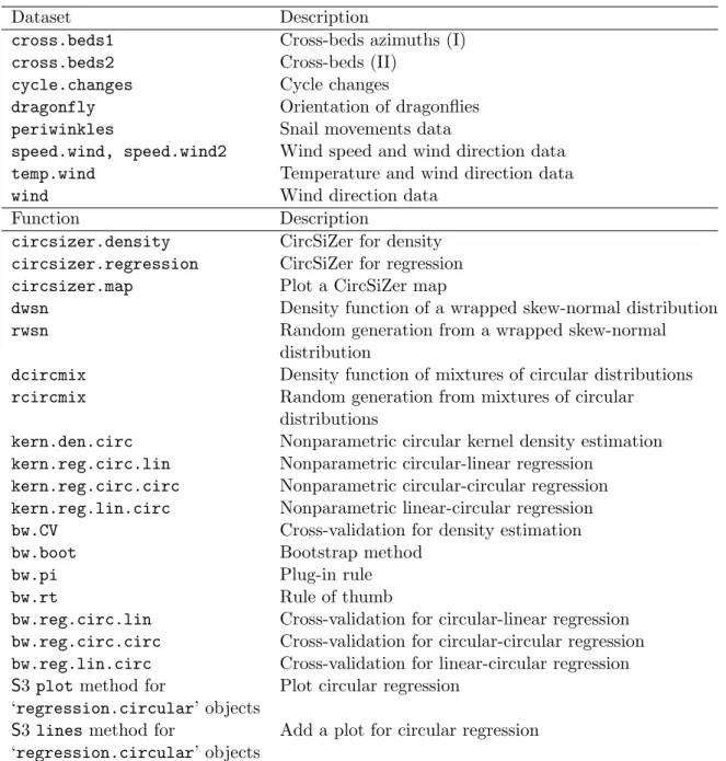
0 π 2 π 3π 2 + ● ● ● ● ● ● ● ● ● ● ● ● ● ● ● ● ● ● ● ● ● ● ● ● ● ● ● ● ● ● ● ● ● ● ● ● ● ● ● ● ● ● ● ● ● ● ● ● ● ● ● ● ● ● ● ● ● ● ● ● ● ●● ● ● ● ●● ● ● ● ● ● ● ● ●● ● ● ● ● ● ● ● ●_● ● ● ● ● ● ● ● ● ● ● ● ● ● ● 0 π 2 π 3π 2 + ● ● ● ● ● ● ● ● ● ● ● ● ● ● ● ● ● ● ● ● ● ● ● ● ● ● ● ● ● ● ● ● ● ● ● ● ● ● ● ● ● ● ● ● ● ● ● ● ● ● ● ● ● ● ● ● ● ● ● ● ● ● ● ● ● ● ● ● ● ● ● ● ● ● ● ● ● ● ● ● ● ● ● ● ● ● ● ● ● ●● ● ● ● ● ● ● ● ● ●

Figure 1: Left panel: density function (solid line) of the Model 18 fromOliveiraet al. (2012) and a random sample of sizen= 100 (dots on the circle). Right panel: density function (solid line) of the mixture model 0.5·vM(0,5) + 0.5·WSN(π,1,10) and a random sample of size n= 100 (dots on the circle).

Note that argumentxmust be an object of class ‘circular’ (seeLund and Agostinelli 2013). Both the model density curve and the random sample are plotted in Figure 1 (left panel). Functions from the circular package allow to plot the sample over a circle and the circular density as shown in the following lines

R> plot(data18, shrink = 1.2)

R> lines(t, f18, shrink = 1.2, lwd = 2)

which provide Figure 1 (left panel).

Apart from the predefined models fromOliveiraet al.(2012), the density function or a random sample from any mixture model can be obtained by using the same functions by specifying the distributions that participate in the mixture through argument dist and the parameters of each distribution by means of argumentparam. For example, a mixture with equal proportions of a von Mises vM(0,5) and a wrapped skew-normal WSN(π,1,10) can be obtained with the code:

R> fmix <- dcircmix(x = t, model = NULL, dist = c("vm", "wsn"), + param = list(p = c(0.5, 0.5), mu = c(0, pi), con = c(5, 1), + sk = c(0, 10)))

and random deviates from the same model can be obtained by:

R> datamix <- rcircmix(100, model = NULL, dist = c("vm","wsn"), + param = list(p = c(0.5, 0.5), mu = c(0, pi), con = c(5, 1), + sk = c(0, 10)))

The corresponding density function and random sample are shown in Figure1 (right panel). Function kern.den.circ

Functionkern.den.circcomputes the circular kernel density estimator with von Mises kernel (Equation 3), for the data sample specified by argument x (the object is coerced to class

(13)

‘circular’) and with a smoothing parameter included in argumentbw. Unless the argument

tis provided, the estimator is computed over a grid of points specified by argumentsfrom,to

andlenwith default values,from = circular(0),to = circular(2 * pi)andlen = 250. If no value of the smoothing parameter is provided by the user the circular kernel estimator is computed with the value of the smoothing parameter selected by the plug-in rule. The output of this function is an object of class ‘density.circular’ (see Lund and Agostinelli 2013) whose underlying structure is a list containing the following components among others:

data, the original dataset; x, the points where the density is estimated; y, the estimated density values;bw, the smoothing parameter used.

For a sample of 200 data from Model 7 fromOliveiraet al.(2012), the circular kernel density estimator can be obtained as follows:

R> data7 <- rcircmix(200, model = 7)

R> est7 <- kern.den.circ(x = data7, t = NULL, bw = 20, from = circular(0), + to = circular(2 * pi), len = 250)

R> est7

Call:

kern.den.circ(x = data7, t = NULL, bw = 20, from = circular(0), to = circular(2 * pi), len = 250)

Data: data7 (200 obs.); Bandwidth 'bw' = 20

x y

n : 2.500e+02 Min. :0.01046

Min. :-3.129e+00 1st Qu.:0.04689 1st Qu.:-1.558e+00 Median :0.12702 Median : 0.000e+00 Mean :0.16015 Mean :-1.959e-14 3rd Qu.:0.26730 3rd Qu.: 1.558e+00 Max. :0.42007 Max. : 3.129e+00

Rho : 4.000e-03

R> names(est7)

[1] "data" "x" "y" "bw" "n" "kernel" [7] "call" "data.name" "has.na"

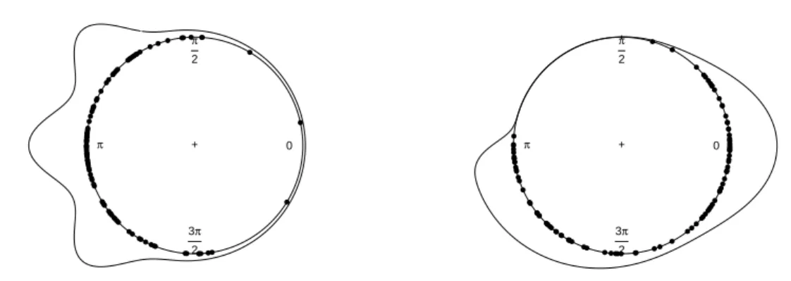
Theprintmethod for ‘density.circular’ objects from packagecircularuses the output of

kern.den.circto provide summaries of the estimation, as can be seen in the example. The graphical display of the estimator is shown in Figure2. Circular and linear representations are displayed in left and right panels, respectively. The solid black line is the true underlying density and the red curve is the circular kernel density estimator. These plots are obtained by using theplot methods for ‘density.circular’ objects from packagecircular. Alines

method for ‘density.circular’ objects from package circular can be also used for adding other estimates to the plot.

(14)

N = 200 Bandwidth = 20 Unit = radians Density circular 0 π 2 π 3π 2 + ● ● ● ● _● ● ● ● ● ● ● ● ● ● ● ● ● ● ● ● ● ● ● ● ● ● ● ● ● ● ● ● ● ● ● ● ● ● ● ● ● ●● ● ● ● ● ● ● ● ● ● ● ● ● ● ● ● ● ● ● ● ● ● ● ● ● ● ● ● _● ● ● ● ● ● ● ● ● ● ● ● ● ● ● ● ● ● ● ● ● ● ● ● ● ● ● ● ● ● ● ● ● ● ● ● ● ● ● ● ● ● ● ● ● ● ● ● ● ● ● ● ● ● ● ● ● ● ● ● ● ● ● ● ● ● ● ● ● ● ● ● ● ● ● ● ● ● ● ● ● ● ● ● ● ● ● ● ● ● ● ● ● ● ● ● ● ● ● ● ● ● ● ● ● ● ● ● ● ● ● ● ● ● ● ● ● ● ● ● ● ● ● ● ● ● ● ● ● ● 0 1 2 3 4 5 6 0.0 0.1 0.2 0.3 0.4

N = 200 Bandwidth = 20 Unit = radians

Density circular ● ● ● ● ● ● ● ●● ●●●●●●● ●● ●●●●●●●●●●● ● ● ●●●●●●●●●●●●● ● ● ● ● ●●●●●●●●●●●●●● ●●●● ● ● ● ●●●●● ●● ● ●●● ●●● ●●●●●●● ●●●●●●●●●●●●● ● ●●●●●●●●●●●●●●●●●●●●●●●●●●●●●●●●●●●●●●●●●●●●●●●●●●●●● ●●●●●●●●● ●● ●●●●●●●●●●●●●●●●●●●●●●●●● ●● ● ● ● ● ●

Figure 2: Circular (left panel) and linear (right panel) representation of the circular kernel density estimator withν = 20 (red line) of a sample of size 200 from Model 7 inOliveiraet al. (2012) and true density (black line).

The value of the parameter bw in function kern.den.circ can also be selected by some of the other rules defined in Section 2.1. The available procedures for choosing the smoothing parameter will be described below. The main argument in all the functions is the data from which the smoothing parameter is to be computed, denoted by x. As before, the object is coerced to class ‘circular’.

Functionbw.bootimplements the bootstrap procedure proposed byMarzioet al.(2011). The minimum of the bootstrap MISE is obtained by using theoptimize function from package stats, which searches the minimum in the interval specified by arguments lower and upper

(default values are 0 and 50, respectively) and with accuracy specified bytol (default: tol = 0.1). The integral is approximated by a sum of np = 500terms.

R> bw.boot(x = data7)

[1] 14.68244

Cross-validation smoothing parameters for density estimation are computed by functionbw.CV. The cross-validation rule to be used, LSCV or LCV, will be specified by argument method, taking LCV as default. When the LSCV smoothing parameter is computed, the integral term in Equation 8 is calculated using the Simpson’s rule (through an internal function) and so, the argumentnpwill be used. As before, the minimum/maximum is searched withoptimize

according to argumentslower,upperand tol.

R> bw.CV(x = data7, method = "LCV")

[1] 16.47961

(15)

[1] 15.91682

Function bw.pi implements the von Mises scale plug-in rule defined by Steps 1–3 in Sec-tion 2.1. Two options are available: fix the number of components in the mixture (denoted byM in Equation 2) by specifying argument M:

R> bw.pi(x = data7, M = 3)

[1] 26.4165

or select the number of components by AIC (default option):

R> bw.pi(x = data7, outM = TRUE)

[1] 25.86334 2.00000

Argument outM = TRUE indicates that the function also returns the number of components in the mixture. Again, the integral term is approximated by the Simpson’s rule and the minimum is searched by using the function optimize.

Finally, the selector proposed byTaylor(2008) for density estimation is computed by function

bw.rt. This selector is based on an estimation of the concentration parameter of a von Mises distribution. The concentration parameter can be estimated by maximum likelihood (robust = FALSE):

R> bw.rt(x = data7, robust = FALSE)

[1] 0.1919247

or by the robustified procedure described before, by setting robust = TRUE. In this case, the argument alphamust be also specified:

R> bw.rt(x = data7, robust = TRUE, alpha = 0.5)

[1] 2.218956

Function circsizer.density

The CircSiZer map for density estimation is provided by circsizer.density. The main arguments in this function are x, the angle data sample (object of class ‘circular’) and

bws, a grid of positive smoothing parameters. Other arguments can be fixed: ngrid, integer indicating the number of equally spaced angles between 0 and 2πwhere the estimator is evalu-ated (default: ngrid = 250);alpha, the significance level for assessing increasing/decreasing patterns (default: alpha = 0.05);B, the number of bootstrap samples to estimate the stan-dard deviation of ˆf0(θ;ν) (default: B = 500); log.scale, logical indicating if the values of the smoothing parameter are transformed to −log₁₀ scale; and display, logical indicating if the CircSiZer map is plotted. This function returns an object of class ‘circsizer’ whose

(16)

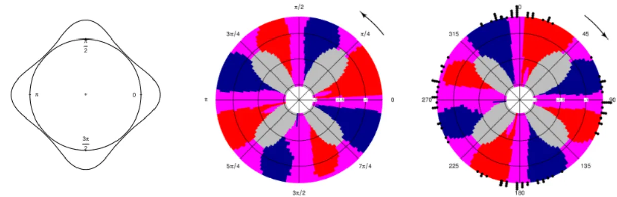
0 π 2 π 3π 2 +

Figure 3: Density for Model 14 from Oliveira et al. (2012) (left panel) and CircSiZer map for kernel density estimator (right panel) based on 100 simulated data (dots over the circle). Peaks and valleys are identified by clockwise blue-red and red-blue patterns, respectively.

underlying structure is a list containing the following components: data, the original dataset;

ngrid, the number of equally spaced angles where the derivative of the circular kernel density estimator is evaluated where the density is estimated,bw, a vector of smoothing parameters (given in −log₁₀ scale if log.scale = TRUE); log.scale, logical indicating if −log₁₀ scale is used for constructing the CircSiZer map; CI, a list containing three matrices where each row corresponds to a value of the smoothing parameter and each column corresponds to an angle: a matrix with lower limits of the confidence intervals, a matrix with the upper limits of the confidence intervals and a matrix with the effective sample size for each pair smoothing parameter-angle; and col, matrix containing the colors for plotting the CircSiZer map. As for the previous matrices, each entry contains the corresponding color for a pair of smoothing parameter-angle.

The CircSiZer map in Figure3is obtained with the following code lines:

R> data14 <- rcircmix(100, model = 14)

R> circsizer14 <- circsizer.density(data14, bws = seq(0, 100, by = 5), + ngrid = 250, alpha = 0.05, B = 500, log.scale = TRUE, display = TRUE) R> names(circsizer14)

[1] "data" "ngrid" "bw" "log.scale" "CI" "col" [7] "call" "data.name"

As noted before, in a CircSiZer map (see Figure 3), blue color indicates locations where the curve is significantly increasing; red color shows where it is significantly decreasing and purple indicates where it is not significantly different from zero. Thus, for a given smoothing parameter, a significant peak can be identified when a region of significant positive gradient is followed by a region of significant negative gradient (i.e., blue-red pattern), and a significant trough by the reverse (red-blue pattern), taking as sense of rotation the direction marked by the arrow. Values of the smoothing parameter are indicated along the radius, transformed to−log₁₀ scale for log.scale = TRUE (default option). Hence, in Figure 3, the multimodal structure of the Model 14 fromOliveira et al. (2012) is clearly brought out by the CircSiZer map.

(17)

Ifdisplay = FALSE, the CircSiZer map is not produced. However, the CircSiZer map can be plotted later by using the functioncircsizer.map whose main argument must be an object of classcircsizer. This function allows to edit the graph by specifying the argumentstype,

zero,clockwise,title,labels,label.pos,rad.posandraw.datawhich allow to indicate the zero of the plot, the sense of rotation, the title, the labels and their position, the position of the radial lines and if the original data is plotted. For the above example, the code

R> circsizer.map(circsizer14, type = 4, zero = pi/2, clockwise = TRUE, + raw.data = TRUE)

provides the CircSiZer map but edited in another way (see Figure3, right panel).

3.3. Illustration for regression estimation

For regression estimation with circular variables, NPCirc includes the following functions:

kern.reg.circ.lin, kern.reg.circ.circ and kern.reg.lin.circ which allow to com-pute the local linear and Nadaraya-Watson estimators for circular-linear, circular-circular and linear-circular data, respectively. NPCircalso includes three functions for computing the cross-validation smoothing parameter in each case: bw.reg.circ.lin, bw.reg.circ.circ

andbw.reg.lin.circ. Finally, circsizer.regressionallows to obtain the CircSiZer map for the regression setting when the covariate is circular and the response is linear.

Functionskern.reg.circ.lin, kern.reg.circ.circ and kern.reg.lin.circ

Functions kern.reg.circ.lin, kern.reg.circ.circ and kern.reg.lin.circ implement the local linear estimator and the Nadaraya-Watson estimator for circular-linear data (circular covariate and linear response), circular-circular data (circular covariate and circular response) and linear-circular data (linear covariate and circular response), respectively. The arguments in these functions are: x, the vector of data for the independent variable; y, the vector of data for the dependent variable;t, the points where to evaluate the estimator; bw, the value of the smoothing parameter to be used; method, a character string giving the estimator to be used. This must be one of "LL" for local linear estimator or"NW" for Nadaraya-Watson estimator. These functions return an object of class ‘regression.circular’ with a list structure containing, among others, the following components: data the original dataset; x, the points where the regression function is estimated; y, the estimated values; and bw, the smoothing parameter used.

For each function, the value of the smoothing parameter can be set manually or can be obtained by calling (default option) the functionsbw.reg.circ.lin,bw.reg.circ.circand

bw.reg.lin.circ, respectively. These functions provide the least squares cross-validation smoothing parameter for the Nadaraya-Watson and local linear estimators. For circular-linear data, the smoothing parameter is selected as the value that minimizes Equation 12. For circular-circular and linear-circular regression, minimization of Equations13or14provide smoothing parameters, the method in Equation13 being the default option. The arguments

x,yand method of this function have the same meaning as before.

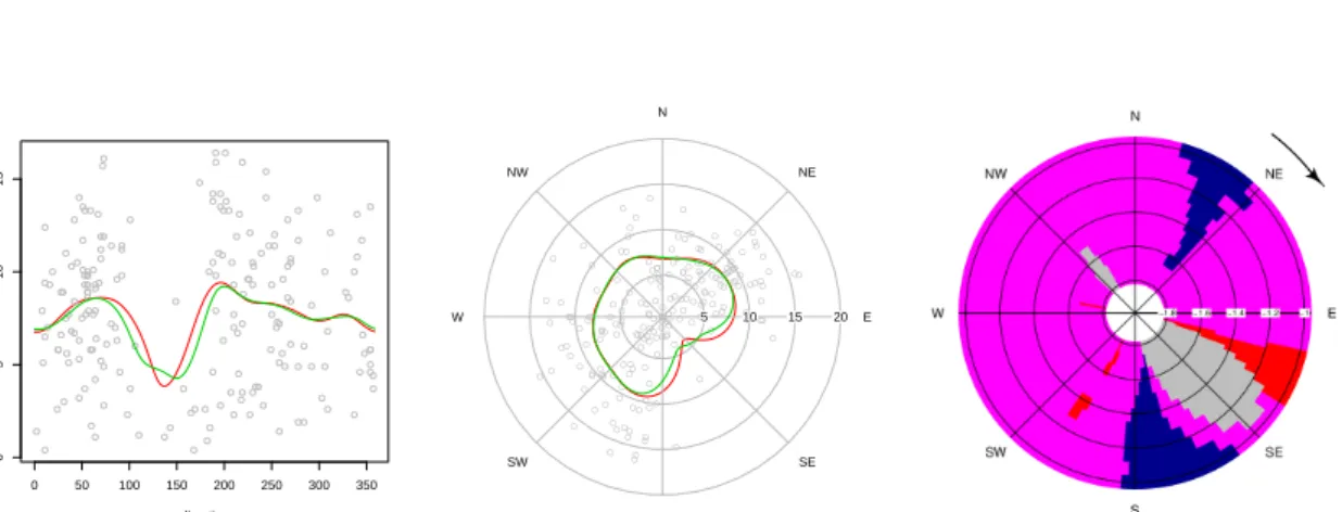
Functions kern.reg.circ.lin and bw.reg.circ.lin are illustrated with the wind.speed

dataset. The Nadaraya-Watson and local linear estimators for a regression model of wind speed over wind direction are shown in Figure4(left panel), in red and green lines respectively. Estimators are obtained with the code:

(18)

R> data("speed.wind2", package = "NPCirc") R> dir <- speed.wind2$Direction

R> vel <- speed.wind2$Speed R> nas <- which(is.na(vel))

R> dir <- circular(dir[-nas], units = "degrees") R> vel <- vel[-nas]

R> bw.reg.circ.lin(dir, vel, method = "LL")

[1] 9.058419

R> bw.reg.circ.lin(dir, vel, method = "NW")

[1] 12.6612

R> estLL <- kern.reg.circ.lin(dir, vel, method = "LL"); estLL

Call:

kern.reg.circ.lin(x = dir, y = vel, method = "LL") Data: dir (199 obs.); Bandwidth 'bw' = 9.058

x y

n : 2.500e+02 Min. :4.265

Rho : 4.000e-03

> estNW <- kern.reg.circ.lin(dir, vel, method = "NW"); estNW

Call:

kern.reg.circ.lin(x = dir, y = vel, method = "NW") Data: dir (199 obs.); Bandwidth 'bw' = 12.66

x y

n : 2.500e+02 Min. :3.836

(19)

0 50 100 150 200 250 300 350 0 5 10 15 direction speed (m/s) ● ● ● ● ● ● ● ● ● ● ● ● ● ● ● ● ● ● ● ● ● ● ● ● ● ● ● ● ● ● ● ● ● ● ● ● ● ● ● ● ● ● ● ● ● ● ● ● ● ● ● ● ● ● ● ● ● ● ● ● ● ● ● ● ● ● ● ● ● ● ● ● ● ● ● ● ● ● ● ● ● ● ● ● ● ● ● ● ● ● ● ● ● ● ● ● ● ● ● ● ● ● ● ● ● ● ● ● ● ● ● ● ● ● ● ● ● ● ● ● ● ● ● ● ● ● ● ● ● ● ● ● ● ● ● ● ● ● ● ● ● ● ● ● ● ● ● ● ● ● ● ● ● ● ● ● ● ● ● ● ● ● ● ● ● ● ● ● ● ● ● ● ● ● ● ● ● ● ● ● ● ● ● ● ● ● ● ● ● ● ● ● ● ● ● ● ● ● ● N NE E SE S SW W NW 5 10 15 20 ● ● ● ● ● ● ● ● ● ● ● ● ● ● ● ● ● ● ● ● ● ● ● ● ● ● ● ● ● ● ● ● ● ● ● ● ● ● ● ● ● ● ● ● ● ● ● ● ● ● ● ● ● ● ● ● ● ● ● ● ● ● ● ● ● ● ● ● ● ● ● ● ● ● ● ● ● ● ● ● ● ● ● ● ● ● ● ● ● ● ● ● ● ● ● ● ● ● ● ● ● ● ● ● ● ● ● ● ● ● ● ● ● ● ● ● ● ● ● ● ● ●● ● ● ● ● ● ● ● ● ● ● ● ● ● ● ● ● ● ● ● ● ● ● ● ● ● ● ● ● ● ● ● ● ● ● ● ● ● ● ● ● ● ● ● ● ● ● ● ● ● ● ● ● ● ● ● ● ● ● ● ● ● ● ● ● ● ● ● ● ● ● ● ● ● ● ● ●

Figure 4: Left and center: linear and circular representations of the Nadaraya-Watson estima-tor (red line) and local linear estimaestima-tor (green line) with cross-validation smoothing parameter for wind speed (m/s) with respect to wind direction. Right: CircSiZer map for circular-linear regression for wind speed (m/s) with respect to wind direction.

The objects (estNW and estLL), of class regression.circular, contain useful information such as the original data, the fitted values or the smoothing parameter. This information is used in the print method for ‘regression.circular’ objects to show summaries of the fitted model and in theplot andlines methods for ‘regression.circular’ objects, which allow to plot the regression estimates. The following code lines produce the plots represented in Figure4 (left and center):

R> plot(estNW, plot.type = "line", points.plot = TRUE, lwd = 2, line.col = 2, + xlab = "direction", ylab = "speed (m/s)")

R> lines(estLL, plot.type = "line", lwd = 2, line.col = 3) R> res <- plot(estNW, plot.type = "circle", points.plot = TRUE, + labels = c("N", "NE", "E", "SE", "S", "SO", "O", "NO"), + label.pos = seq(0, 7 * pi/4, by = pi/4),

+ zero = pi/2, clockwise = TRUE, lwd = 2, line.col = 2, main = "") R> lines(estLL, plot.type = "circle", plot.info = res, lwd = 2,

+ line.col = 3)

Ifplot.type = "line", a linear representation of the estimator is obtained. The periodicity can be appreciated by joining the extremes of the lines. A circular representation can be produced by settingplot.type = "circle".

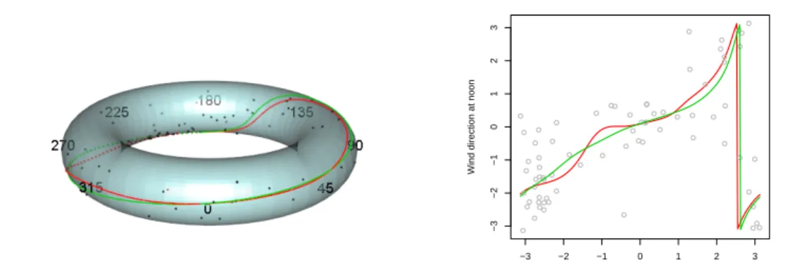
Functionskern.reg.circ.circandbw.reg.circ.circare illustrated with thewinddataset. The circular-circular regression estimator is used to model the wind direction at noon, based on the wind direction at 6 a.m. (see Marzio et al. 2012). The argument option indicates the cross-validation function to be used for selecting the smoothing parameter. Ifoption = 1 (default option), then the criterion in Equation 13 is considered whereas if option = 2, Equation14 is used:

R> data("wind", package = "NPCirc")

R> wind6 <- circular(wind$wind.dir[seq(7, 1752, by = 24)]) R> wind12 <- circular(wind$wind.dir[seq(13, 1752, by = 24)])

(20)

−3 −2 −1 0 1 2 3 −3 −2 −1 0 1 2 3

Wind direction at 6 a.m.

Wind direction at noon

● ● ● ● ● ● ● ● ● ● ● ● ● ● ● ● ● ● ● ● ● ● ●● ● ● ● ● ● ● ● ● ● ● ● ● ● ● ● ● ● ● ● ● ● ● ● ● ● ● ● ● ● ● ● ● ● ● ● ● ●● ● ● ● ● ● ● ● ● ● ● ●

Figure 5: Representation on the torus (left panel) and linear representation (right panel) of Nadaraya-Watson (red line) and local linear (green line) estimators for wind directions at noon with respect to wind directions at 6 a.m.

R> bw.reg.circ.circ(wind6, wind12, method = "LL", option = 1, + lower = 0, upper = 20)

[1] 2.834813

R> bw.reg.circ.circ(wind6, wind12, method = "NW", option = 1, lower = 0, + upper = 20)

[1] 5.482274

R> bw.reg.circ.circ(wind6, wind12, method = "LL", option = 2, lower = 0, + upper = 20)

[1] 2.252278

R> bw.reg.circ.circ(wind6, wind12, method = "NW", option = 2, lower = 0, + upper = 20)

[1] 6.080389

R> estNW <- kern.reg.circ.circ(wind6, wind12, t = NULL, bw = 6.1, + method = "NW")

R> estLL <- kern.reg.circ.circ(wind6, wind12, t = NULL, bw = 2.25, + method = "LL")

For circular-circular regression, the estimates can be plotted on a torus, by settingplot.type = "circle"with the following code:

R> plot(estNW, plot.type = "circle", points.plot = TRUE, line.col = 2, + lwd = 2, points.col = 1, units = "degrees")

(21)

0 20 40 60 80 100 120 50 100 150 200 Distance (cms) Direction (degrees) ● ● ● ●● ● ● ● ● ● ● ● ● ● ● ● ● ● ● ● ● ● ● ● ● ● ● ● ● ● ●

Figure 6: Representation on the cylinder (left panel) and linear representation (right panel) of the Nadaraya-Watson (red line) and local linear (green line) estimators for theperiwinkle

data.

yielding the left plot in Figure5. It should be noted that this is a 3D plot that can be rotated to explore the characteristics of the fitted curve. To produce this graphic, packagesmisc3d(Feng and Tierney 2008) and rgl (Adler, Murdoch et al. 2014) are needed. Nevertheless, a linear representation is also possible (plot.type = "line"). The linear plot of the observations at 6 a.m. and noon, together with the Nadaraya-Watson and local-linear estimators are shown in Figure5 (right) which have been obtained with the following code lines:

R> plot(estNW, plot.type = "line", points.plot = TRUE, line.col = 2, lwd = 2, + xlab = "Wind direction at 6 a.m.", ylab = "Wind direction at noon") R> lines(estLL, plot.type = "line", line.col = 3, lwd = 2)

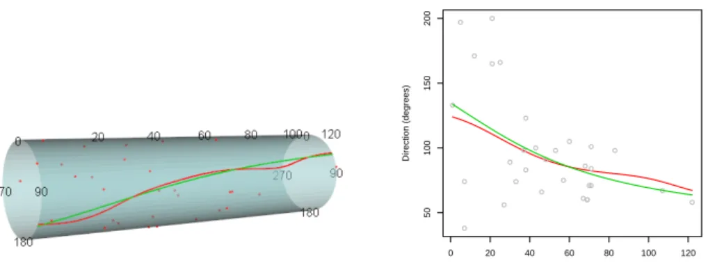
Finally, functionskern.reg.lin.circandbw.reg.lin.circare illustrated with the dataset

periwinkle. In this case, the linear-circular estimators are used to model the angles with regard to the distance moved:

R> data("periwinkles", package = "NPCirc") R> dist <- periwinkles$distance

R> dir <- circular(periwinkles$direction, units = "degrees")

R> bw.reg.lin.circ(dist, dir, method = "NW", option = 1, lower = 0, + upper = 50)

[1] 21.24758

R> bw.reg.lin.circ(dist, dir, method = "NW", option = 2, lower = 0, + upper = 50)

[1] 21.50279

R> estNW <- kern.reg.lin.circ(dist, dir, t = NULL, bw = 21.25, + method = "NW")

(22)

For linear-circular regression, the estimates can be plotted on a cylinder (see Figure 6, left panel), by settingplot.type = "circle"with the following code:

R> plot(estNW, plot.type = "circle", points.plot = TRUE, line.col = 2, + lwd = 2, points.col = 2)

R> lines(estLL, plot.type = "circle", line.col = 3, lwd = 2)

A linear representation of the estimators is shown in Figure6 (right panel). Function circsizer.regression

The functioncircsizer.regressionprovides the CircSiZer map for regression, considering a circular covariate and a linear response. The first arguments for this function are x, the data for the circular covariate and y, the data for the dependent linear variable y. The remaining arguments are the same as for function circsizer.density. If argument bws is not specified (bws = NULL), a CircSiZer map for regression is, by default, computed for two values of the smoothing parameter. These two values are selected according to the value of the smoothing parameter provided by the corresponding least squares cross-validation rule and the parameter adjust(by defaultadjust = 2). Thus, the CircSiZer map is obtained for the values bw/adjust and bw * adjust.

Figure4(right panel) shows the CircSiZer map for exploring the relation between wind speed as a response and wind direction as a covariate, obtained with the code:

R> circsizer <- circsizer.regression(dir, speed, bws = seq(10, 60, by = 5), + display = FALSE)

R> circsizer.map(circsizer, type = 1, zero = pi/2, clockwise = TRUE)

In the CircSiZer map, it can be seen that wind speed increases when wind direction comes from NE and S-SW and winds from SE are not frequent at all, this fact being reflected by the gray colored area.

As for the density setting, the output of the functioncircsizer.regressioncan be provided as the first argument of functioncircsizer.map in order to obtain a new CircSiZer map.

4. Conclusion and extensions

In this paper, theNPCircpackage for performing nonparametric density and regression esti-mation with circular data inRis described, illustrating its performance with simulated and real data examples. Thus, the packageNPCirccontains functions for computing the nonpara-metric kernel circular density estimator and circular-linear, circular-circular and linear-circular regression estimators, which provide several useful tools for analyzing circular data without imposing parametric constraints. Moreover, for choosing a smoothing parameter, different selectors, both for density and regression, have been revised and a graphical tool has been proposed in order to avoid the smoothing parameter selection and explore the estimators at different smoothing levels.

Circular data appear in a variety of disciplines and so, this package can be of interest to nonparametric practitioners of different scientific fields.

(23)

In this current version, package NPCirc includes nonparametric methods based on the von Mises kernel. Different kernels or even, another kind of smoothers such as periodic splines could be considered in order to extend the package.

Acknowledgments

The authors want to acknowledge two anonymous referees for their comments which helped in improving both the paper and the package contents. The authors also acknowledge Prof. A. Pewsey for providing the dragonflies and cross beds data. Data from periglacial, collected within the Project POL2006–09071 from the Spanish Ministry of Education and Science have been provided by Prof. A. P´erez-Alberti. Data stored in the wind dataset are provided by NCAR/EOL under the sponsorship of the National Science Foundation.

This research has been supported by Project MTM2008–03010 from the Spanish Ministry of Science and Innovation, and by the IAP network StUDyS (Developing crucial Statistical methods for Understanding major complex Dynamic Systems in natural, biomedical and social sciences), from Belgian Science Policy.

References

Abe T, Pewsey A (2011). “Symmetric Circular Models Through Duplication and Cosine Perturbation.”Computational Statistics & Data Analysis,55(12), 3271–3282.

Adler D, Murdoch D,et al.(2014).rgl: 3D Visualization Device System (OpenGL).Rpackage version 0.94.1131, URL http://CRAN.R-project.org/package=rgl.

Bai ZD, Rao CR, Zhao LC (1988). “Kernel Estimators of Density Function of Directional Data.”Journal of Multivariate Analysis,27(1), 24–39.

Banerjee A, Dhillon IS, Ghosh J, Sra S (2005). “Clustering on the Unit Hypersphere Using von Mises-Fisher Distributions.” Journal of Machine Learning Research, 6(September), 1345–1382.

Barrag´an S, Fern´andez MA (2014). isocir: Isotonic Inference for Circular Data. R package version 1.1-3, URLhttp://www.CRAN.R-project.org/package=isocir.

Batschelet E (1981). Circular Statistics in Biology. Academic Press, New York.

Bowers JA, Morton ID, Mould GI (2000). “Directional Statistics of the Wind and Waves.” Applied Ocean Research,22(1), 13–30.

Brunsdon C, Corcoran J (2005). “Using Circular Statistics to Analyse Time Patterns in Crime Incidence.” Computers, Environment and Urban Systems,30(3), 300–319.

Chaudhuri P, Marron JS (1999). “SiZer for Exploration of Structures in Curves.”Journal of the American Statistical Association,94(447), 807–823.

(24)

Feng D, Tierney L (2008). “Computing and Displaying Isosurfaces inR.”Journal of Statistical Software,28(1), 1–24. URL http://www.jstatsoft.org/v28/i01/.

Fern´andez-Dur´an JJ, Gregorio-Dom´ınguez MM (2013). CircNNTSR: AnRPackage for the Statistical Analysis of Circular Data Using Nonnegative Trigonometric Sums (NNTS) Mod-els. Rpackage version 2.1, URLhttp://www.CRAN.R-project.org/package=CircNNTSR. Fisher NI (1993). Statistical Analysis of Circular Data. Cambridge University Press,

Cam-bridge.

Fisher NI, Lee AJ (1992). “Regression Models for Angular Responses.” Biometrics, 48(3), 665–677.

Hall P, Watson GP, Cabrera J (1987). “Kernel Density Estimation for Spherical Data.” Biometrika,74(4), 751–762.

Hornik K, Gr¨un B (2014). “movMF: An R Package for Fitting Mixtures of von Mises-Fisher Distributions.”Journal of Statistical Software,58(10), 1–31. URLhttp://www.jstatsoft.

org/v58/i10/.

Jammalamadaka SR, Lund UJ (2006). “The Effect of Wind Direction on Ozone Levels: A Case Study.”Environmental and Ecological Statistics,13(3), 287–298.

Jammalamadaka SR, SenGupta A (2001). Topics in Circular Statistics. World Scientific, Singapore.

Jones MC, Pewsey A (2012). “Inverse Batschelet Distributions for Circular Data.”Biometrics,

68(1), 183–193.

Kato S, Shimizu K, Shieh G (2008). “A Circular-Circular Regression Model.”Statistica Sinica,

18(2), 633–645.

Klemel¨a J (2000). “Estimation of Densities and Derivatives of Densities with Directional Data.”Journal of Multivariate Analysis,73(1), 18–40.

Lund U, Agostinelli C (2012). CircStats: Circular Statistics, from ‘Topics in Circular Statis-tics’ (2001). R package version 0.2-4, URL http://www.CRAN.R-project.org/package=

CircStats.

Lund U, Agostinelli C (2013). circular: Circular Statistics. R package version 0.4-7, URL

http://www.CRAN.R-project.org/package=circular.

Mann KA, Gupta S, Race A, Miller MA, Cleary RJ (2003). “Application of Circular Statistics in the Study of Crack Distribution Around Cemented Femoral Components.” Journal of Biomechanics,36(8), 1231–1234.

Mardia KV (1972). Statistics of Directional Data. Academic Press, New York. Mardia KV, Jupp PE (2000). Directional Statistics. John Wiley & Sons, New York.

Marzio MD, Panzera A, Taylor CC (2009). “Local Polynomial Regression for Circular Pre-dictors.”Statistics & Probability Letters,79(19), 2066–2075.

(25)

Marzio MD, Panzera A, Taylor CC (2011). “Kernel Density Estimation on the Torus.”Journal of Statistical Planning & Inference,141(6), 2156–2173.

Marzio MD, Panzera A, Taylor CC (2012). “Non-Parametric Regression for Circular Re-sponses.”Scandinavian Journal of Statistics,40(2), 238–255.

Mooney JA, Helms PJ, Jollife IT (2003). “Fitting Mixtures of von Mises Distributions: A Case Study Involving Sudden Infant Death Syndrome.” Computational Statistics & Data Analysis,41(3–4), 505–513.

Oliveira M, Crujeiras RM, Rodr´ıguez-Casal A (2012). “A Plug-in Rule for Bandwidth Selection in Circular Density Estimation.”Computational Statistics & Data Analysis,56(12), 3898– 3908.

Oliveira M, Crujeiras RM, Rodr´ıguez-Casal A (2013). “Nonparametric Circular Methods for Exploring Environmental Data.”Environmental and Ecological Statistics,20(1), 1–17. Oliveira M, Crujeiras RM, Rodr´ıguez-Casal A (2014a). “CircSiZer: An Exploratory Tool for

Circular Data.”Environmental and Ecological Statistics,21(1), 143–159.

Oliveira M, Crujeiras RM, Rodr´ıguez-Casal A (2014b). NPCirc: Nonparametric Circu-lar Methods. R package version 2.0.1, URL http://www.CRAN.R-project.org/package=

NPCirc.

Parzen E (1962). “On Estimation of a Probability Density Function and Mode.”The Annals of Mathematical Statistics,33(3), 1065–1076.

Pewsey A (2000). “The Wrapped Skew-Normal Distribution on the Circle.”Communications in Statistics – Theory and Methods,29(11), 2459–2472.

Presnell B, Morrison SP, Littel RC (1998). “Projected Multivariate Linear Models for Direc-tional Data.”Journal of the American Statistical Association,93(443), 1068–1077.

RCore Team (2014). R: A Language and Environment for Statistical Computing. R Founda-tion for Statistical Computing, Vienna, Austria. URLhttp://www.R-project.org/. Qin X, Zhang JS, Yan XD (2011a). “Local Linear Least Squares Kernel Regression for Linear

and Circular Predictors.” Communications in Statistics – Theory and Methods, 40(21), 3812–3823.

Qin X, Zhang JS, Yan XD (2011b). “A Nonparametric Circular-Linear Multivariate Regres-sion Model with a Rule-of-Thumb Bandwidth Selector.” Computers & Mathematics with Applications,62(8), 3048–3055.

Rosenblatt M (1956). “Remarks on Some Nonparametric Estimate of a Density Function.” The Annals of Mathematical Statistics,27(3), 832–837.

SenGupta A, Ugwuowo FI (2006). “Asymmetric Circular-Linear Multivariate Regression Mod-els with Applications to Environmental Data.” Environmental and Ecological Statistics,

(26)

SenGupta S, Rao JS (1966). “Statistical Analysis of Cross-Bedding Azimuths from the Kamthi Formation around Bheemaram, Pranhita: Godavari Valley.”Sankhy¯a: The Indian Journal of Statistics B,28(1/2), 165–174.

Taylor CC (2008). “Automatic Bandwidth Selection for Circular Density Estimation.” Com-putational Statistics & Data Analysis,52(7), 3493–3500.

von Mises R (1918). “ ¨Uber die “Ganzzahligkeit” der Atomgewichte und verwandte Fragen.” Physikalische Zeitschrift,19, 490–500.

Affiliation:

Mar´ıa Oliveira, Rosa M. Crujeiras, Alberto Rodr´ıguez-Casal Department of Statistics and Operations Research

Faculty of Mathematics

University of Santiago de Compostela Spain

E-mail: [email protected],[email protected],

[email protected]