Testing goodness of fit for the distribution of errors in multivariate linear models

(1)

Testing goodness of ﬁt for the distribution of errors

in multivariate linear models

M.D. Jiménez Gamero

a,∗

, J. Muñoz García

a

, R. Pino Mejías

a,b a_{Dpto. Estadística e Investigación Operativa, Facultad de Matematicas C/Tarﬁa s.n. Universidad de Sevilla,}

Spain

b_{Centro Andaluz de Prospectiva, Spain}

Received 21 October 2002 Available online 28 September 2004

Abstract

In this paper, to test goodness of ﬁt to any ﬁxed distribution of errors in multivariate linear models, we consider a weighted integral of the squared modulus of the difference between the empirical characteristic function of the residuals and the characteristic function under the null hypothesis. We study the limiting behaviour of this test statistic under the null hypothesis and under alternatives. In the asymptotics, the rank of the design matrix is allowed to grow with the sample size.

Keywords: Linear models; Distribution of errors; Goodness-of-ﬁt; Residuals; Characteristic function

1. Introduction

Classical theory on linear models assume the errors are normally distributed. Some proce-dures derived under this assumption are valid asymptotically in the presence of nonnormal errors, under fairly general conditions, but others do not (see, for example[1]). So, for the methods used to be valid, the distributional assumption on the errors must be checked. In this article we give a test for testing goodness of ﬁt to any ﬁxed distribution of errors in multivariate linear models.

∗_{Corresponding author.}

E-mail address:[email protected](M.D. Jiménez Gamero).

(2)

Lety1, y2, . . . , ynbe n independent (column) observations inRd, for some ﬁxedd1, following the model

y_j =x_j+ε_j1/2_{, j} ₌₁_,₂_{, . . . , n,} ₍₁₎

where the prime denotes transpose, the design variablesx_j ∈Rpare assumed to be nonran-dom,is an unknownp×d-matrix,1/2is the unique symmetric positive deﬁnite squared root of, which is a nonsingular symmetric positive deﬁnite unknownd×d-matrix, and the εj are the d-vectors of errors, with meanE(ε_j)=0 and covariance matrixvar(ε_j)=I_d, 1jn, beingI_dthe identityd×d-matrix. Without loss of generality, we assume that rank(X)=p, withX=(x1x2. . . xn).

Let F be the unknown distribution function of the errors. The problem considered here is testing whether theε_jare from a speciﬁed distribution, that is, testing the hypothesis

H0:F =F0

for some ﬁxed distribution functionF0onRd.

There is a huge literature on testing goodness of ﬁt for independent and identically distributed (i.i.d.) observations. Although we are assuming the errors are i.i.d., they are not observable. To overcome this difﬁculty, one can “estimate” them by the Studentized residuals,

e

j =(yj −xj)ˆ ˆ− 1/2

,

whereˆ andˆ are adequate estimators ofand, respectively, and then apply some of the above-mentioned goodness of ﬁt tests for testingH0toe1, e2, . . . , en. The problem is that thee_jare not i.i.d., and hence the statistical properties of the tests, when applied to the residuals, must be revised.

A wide class of goodness of ﬁt statistics for i.i.d. observations measure the discrepancy between the distribution function in the null hypothesis and the empirical distribution func-tion of the data, that is, they are funcfunc-tions of the empirical process. Some properties of the empirical process of residuals can be found in the book by Koul[22], ford =1, p ﬁxed andF0continuous. Under some conditions, this process has the same asymptotic null dis-tribution as in ordinary location-scale models (see also Pierce and Kopecky [28]). Portnoy [29] and Mammen [26] have also studied this process for p increasing with n. In general, the asymptotic null distribution of this process depends on the unknown true parameter value, its estimator andF0. Bai [2] has used a transformation of this process to get an asymptotically distribution free test statistic.

Another well-known class of goodness of ﬁt statistics for i.i.d. observations are the chi-squared statistics, which are quadratic functions of the difference between the observed and the null expected frequencies in each cell of a partition ofRd. Jiang [20] has studied some properties of a test statistic in this class for testingH0when data follows model (1),d =1,

p is ﬁxed andF0is a continuous distribution function.

Other class of goodness of ﬁt tests for i.i.d. observations from a continuous population, with density functionf (x), consider as test statistic the integrated squared difference be-tween a kernel estimator of the unknown density function and a parametric estimator of f, obtained under the null hypothesis. To our knowledge, the ﬁrst paper proposing a test in

(3)

this class is the one by Bickel and Rosenblatt[5], whose results have been successively extended by Hall [16] and Fan [10,11,13]. Baltagi and Li [3] have extended Fan’s [10] test to the case of a univariate regression model.

Some goodness of fit statistics for i.i.d. observations measure deviations between the empirical characteristic function (e.c.f.) and the characteristic function (c.f.) in the null hypothesis. Examples are the tests proposed by Koutrouvelis [23], Koutrouvelis and Keller-meier [24] and Fan [12] for testing fit to any distribution; for testing normality, the tests in Murota and Takeuchi [27], Hall and Welsh [17], Welsh [32], Csörg˝o [6] make use of some specific properties of the c.f. of the normal law. Another test based on the e.c.f. for testing univariate normality is the proposed by Epps and Pulley [9], that has been extended to the multivariate case by Baringhaus and Henze [4] and to test fit to any multivariate distribution by Jiménez-Gamero et al. [21]. Although the approach followed in [4,9,21] seems to be quite different from that in the above paragraph, the paper by Fan [13] shows that if instead of making the smoothing parameter of the kernel density estimator of f to shrinks to zero as the sample size grows to infinity, we fix its value, then, under some conditions on the kernel function, the bias-corrected statistic proposed by Fan [10] becomes a weighted integrated squared difference between the e.c.f. and a parametric estimator of the population c.f. under the null hypothesis. This fact was also observed by Henze and Wagner [18] for the test statistic considered in Baringhaus and Henze [4].

The aim of this paper is to study the statistical properties of the test in Baringhaus and Henze [4] and Fan [13] for testingH0when observations obey model (1), but unlike these papers and the tests in Jiang [20], Bai [2], Baltagi and Li [3] and Pierce and Kopecky [28] for testingH0, we will not assume thatF0is a continuous population. We will also allow

p to grow with the sample size n. This feature is important because in many applications,

models are used where p is not small compared with n. Allowing p to increase with n is a way of allowing the model to become more complicated as the sample size increases. The restrictions that will be imposed on the rate at which p can increase, suggest restrictions on the complexity of the model for each finite n. As it will be obvious from these restrictions, the obtained results are also valid for p fixed. Another advantage of our approach is that the dimension of the data, d, although fixed, can be arbitrary, that is, we will assume that

d is ﬁxed for some d1. In addition, the assumptions used to derive the properties of the test in this paper are less restrictive than those considered in the above mentioned articles.

Lety1, y2, . . . , ynbe i.i.d. d-vectors with unknown meanand unknown ﬁnite covariance matrix. This situation is a particular case of model (1) withp=1,x_j =1, 1jnand =_{. For testing multivariate normality, Baringhaus and Henze [4] consider the following} test statistic:

n

|cn(t; ˆ,)ˆ −(t)|2dG(t), (2)

withc_n(t; ˆ,)ˆ the e.c.f. of the Studentized residuals,(t)the c.f. of the d-variate normal law with mean 0 and covariance matrixI_d,N_d(0, I_d), dG(t)proportional to|(t)|2dtand for any complex number,z=a+ib, with i=√−1,|z|2=a2+b2. These authors have obtained the limiting null distribution of statistic (2) and have shown that the test that rejects

(4)

[18] and Epps [8] have also analyzed the limiting behaviour of this test under contiguous alternatives.

In this paper we consider statistic (2) withreplaced by the c.f. of the law inH0and

G a general weight function, and study some properties of the test that rejectH0for large values of this statistic, when the observed data follow model (1).

For the i.i.d. case, when the null hypothesis is true and the smoothing parameter converges to zero at certain rate, the bias-corrected statistic in Fan [10] is asymptotically distribution free. Although this is a quite desirable property, the simulations in Fan [10,11] show that the asymptotic null distribution does not provide an accurate approximation to the small and moderate sample distribution of the test statistic. By contrast, if we fix the smoothing pa-rameter the bias-corrected statistic is not asymptotically distribution free, but its asymptotic null distribution gives a good approximation to its finite sample null distribution. Something similar occurs when data obey model (1): the test in Baltagi and Li [3] is asymptotically distribution free but the asymptotic null distribution does not approximate well the finite sample distribution of the test statistic; we will see that the opposite is true for the test pro-posed here which, following Fan [13], can be considered as a fixed smoothing parameter version of the one in Baltagi and Li [3].

The paper is organized as follows. In Section 2 we introduce the test statistic and study some asymptotic properties whenH0is true. Here we derive its asymptotic null distribution and see that, under some conditions, it is the same as in the i.i.d. case. Next section is devoted to the study of the asymptotic nonnull behaviour of the test statistic. We show that, for adequate choices of the weight function G, the test that rejects the null hypothesis for large values of the test statistic is consistent. We also study its behaviour under contiguous alternatives. The results in Sections 2 and 3 assume that the estimators of parameters in model (1) satisfy some conditions. In Section 4, we discuss such assumptions and see that they are not too restrictive, since commonly used estimators satisfy them. In Section 5, we present the results of a simulation experiment to empirically investigate the convergence of null quantiles to the null quantiles in the i.i.d. case. In this section we also present the result of a simulation study to investigate the ﬁnite sample performance of the proposed test and to compare it with the tests in Pierce and Kopecky [28], Bai [2], Baltagi and Li [3] and Jiang [20]. Next section concludes and indicates a possible extension of the obtained results. All proofs are deferred to Section 7.

Before ending this section we introduce some notation and general assumptions: along this article we assume thaty1, y2, . . . , ynare n independent (column) d-vectors, for some ﬁxedd1, following model (1). Let=(,).hasp×d+d(d+1)/2 linear independent components. We denote them by_k, 1kp×d+d(d+1)/2. Byˆ=(ˆ,ˆ)we denote an estimator of. We assume n large enough to ensure that ˆ is positive deﬁnite with probability 1. In the results in next sections, we let n and p→ ∞, soˆ and X should have subindices n and p,ˆ_n,p andX_n,p. To simplify notation we omit these subindices. The hat matrix is denoted byH = (h_jk) = X(XX)−1X,h_j. = h_.j = n_k₌₁h_jk and

h..=nj,k=1hjk.E{(ε)}denotes the expectation of(ε)with respect to F, the unknown distribution function of the errors, that is,E{(ε)} = (ε)dF (ε), where an unspeciﬁed integral denotes integration over the whole spaceRdand:Rd →Rkis any measurable function, for somek ∈ N. For any distribution function onRd different from F, say G,

(5)

EG{(T )}denotes the expectation of(T )with respect to G,E_G{(T )} = (t)dG(t), whereis as before andT =(T1, T2, . . . ., Td)represents a d-dimensional random vector with distribution function G. For any vector a,a_k denotes its kth coordinate, andaits Euclidean norm. 1_nis the vector ofRnwith all its components equal to 1.

2. The test statistic and its asymptotic null distribution

Letc(t)=R(t)+iI (t),c0(t)=R0(t)+iI0(t)andcn(t; ˆ)=Rn(t; ˆ)+iIn(t; ˆ)with

R(t)=cos(tε)dF (ε), I (t)=sin(tε)dF (ε), R0(t)= cos(tε)dF0(ε), I0(t)= sin(tε)dF0(ε), Rn(t; ˆ)= 1_nnj=1cos(tej), In(t; ˆ)= 1_n _n j=1sin(tej).

Let G be a distribution function onRdand(F )=|c(t)−c0(t)|2dG(t). To testH0we consider the test statistic

Vn = |cn(t; ˆ)−c0(t)|2dG(t) = Rn(t; ˆ)−R0(t) 2 dG(t)+ I_n(t; ˆ)−I0(t) 2 dG(t).

In general, the null distribution ofV_nis difﬁcult to obtain. Clearly, it depends on n, p,F0,

G,ˆ and the design matrix X. The dependence on X is the worst drawback, because the use ofV_nas a test statistic would require to tabulate its percentage points for each possible conﬁguration of X. A way to approximate the null distribution ofV_nis by considering its limiting null distribution. Next we derive it and see that, under some conditions onˆ, if H1_n=1_nthen the asymptotic null distribution ofV_ndoes not depend on X. A big number of linear models fulﬁllH1_n =1_n, examples are analysis of variance models, analysis of covariance models, regression models with intercept, etc.

To obtain the asymptotic null distribution ofV_n we proceed in several steps. First and for a general F, we calculate the ﬁrst order Taylor expansion ofc_n(t; ˆ)−c0(t)and obtain the order of the rest (Proposition2.1). Next, we study the consequences of replacing the derivatives in the Taylor expansion ofc_n(t; ˆ)−c0(t)by their expected values (Proposition 2.2) and see that, under some conditions onˆ, the resultant statistic looks like a degree-2

V-statistic (Proposition 2.3). Second, forF =F0, that is, whenH0is true, we show that

nVn = OP(1)(Corollary 2.1) and that ifH1_n =1_n andˆ has an asymptotic expansion that does not depend on X, then the asymptotic null distribution ofnV_nis identical to the one obtained in the i.i.d. case, where by i.i.d. case we meanX = 1_n and = , being the common mean of all observationsy1, y2, . . . , yn(Corollary 2.2). Consequently, the percentage points of the null distribution ofnV_n can be approximated, at least for large samples, by the percentage points in the i.i.d. case.

By Taylor expansion

Rn(t; ˆ) = Rn(t)+*Rn(t; ˆ)+ZR,n(t; ˆ),

(6)

where Rn(t)= 1_nnj=1cos(tεj), In(t)= 1_n _n j=1sin(tεj), *Rn(t; ˆ)=kRn,k(t;)(ˆk−k), *In(t; ˆ)=kIn,k(t;)(ˆk−k), ZR,n(t; ˆ)=k Rn,k(t; ˜)−Rn,k(t;) (ˆk−k), ZI,n(t; ˆ)=k In,k(t; ˜)−In,k(t;) (ˆk−k), withR_n,k(t;)= * *kRn(t;),In,k(t;)= *

*kIn(t;)and˜ =+(1−)ˆ, for some ∈(0,1). Next result gives the order of the difference betweenV_nand the resultant statistic whenZ_R,n(t; ˆ)andZ_I,n(t; ˆ)are omitted. To do this we assume some conditions onˆ. Condition C.1. ˆ =+o_P(n−1/4).

Condition C.2. √1_nn_j₌₁−1/2₍ˆ₋₎_x

j2=oP(1).

Proposition 2.1. If conditions C.1 and C.2 hold andE_G(T4) <∞, then n{Vn−(F )} =nVn,1−(F ) +oP(n1/2Vn,1/12), (3) whereV_n,1= {Rn(t)+*Rn(t; ˆ)−R0(t)}2dG(t)+ {In(t)+*In(t; ˆ)−I0(t)}2dG(t). Let*ER(t; ˆ)=_kE{R_n,k(t;)}(ˆ_k−_k)and*EI (t; ˆ)=_kE{I_n,k(t;)}(ˆ_k− k). Next proposition gives the effect of replacing*R_n(t; ˆ)and*I_n(t; ˆ)by*ER(t; ˆ) and*EI (t; ˆ), respectively, in the expression ofV_n,1. To derive this result we will assume thatˆ can be expressed as follows.

Condition C.3. ˆ =+(XX)−1n_j₌₁x_j{ (ε_j;)+1_nn_k₌₁h_k.(εk;)+_n1n_k₌₁

(εk;)} +B, for some functions ,, : Rd −→ Rd satisfyingE{ _k(ε;)} = 0, E{ 2

k(ε;)}<∞,E{k(ε;)} =0,E{2_k(ε;)}<∞,E{_k(ε;)} =0,E{2_k(ε;)}< ∞, 1kd, for all ﬁnite positive deﬁniteand the randomp×d-matrix B is such that

_n

j=1Bxj2=oP(1).

We will also assume that the hat matrix satisﬁes Huber’s condition and that p can increase at certain rate, as it is expressed in next conditions.

Condition C.4. hmax= sup 1jn

hjj =o(1). Condition C.5. p2/n=o(1).

(7)

Proposition 2.2. If conditions C.3–C.5 hold,E_G(T2) <∞andˆ =+o_P(1), then nVn,1−(F ) =nVn,2−(F ) +oP(n1/2Vn,1/22), (4) whereV_n,2={R_n(t)+*ER(t; ˆ)−R0(t)}2dG(t)+ {In(t)+*EI (t; ˆ)−I0(t)}2dG(t). Next we show that, under some additional conditions onˆ,V_n,2 resembles a degree-2 V-statistic. In addition of condition C.3, we will assume thatˆsatisﬁes the following: Condition C.6. 1/2ˆ−1/2−I_d =1_nn_j₌₁L_j(ε_j;)+S, withL_j(ε;)=(L_j(ε;)_rs), E{Lj(ε;)rs} =0,E{L2_j(ε;)_rs}<∞, 1r, sd, 1jn, andS=o_P(n−1/2).

Proposition 2.3. If conditions C.3 and C.6 hold andE_G(T2) <∞, then nVn,2−(F ) =nVn,3−(F ) +oP(n1/2Vn,1/32), where Vn,3= 1 n2 n j,k=1 q1j(εj;t)q1k(εk;t)dG(t)+ q2j(εj;t)q2k(εk;t)dG(t) , withq1j(ε;t)=cos(tε)+I (t){hj. (ε;)+h_n..hj.(ε;)+h_n..(ε;)}−1/2t+∇R(t) Lj(ε;)t−R0(t),q2j(ε;t)=sin(tε)−R(t){hj. (ε;)+h_n..hj.(ε;)+h_n..(ε;)} −1/2_t_+∇_{I (t)}_L j(ε;)t−I0(t),∇R(t)=(_*t* 1R(t), * *t2R (t), . . . , * *tdR(t))and∇I (t) ₌ (_*t* 1I (t), * *t2I (t), . . . , * *tdI (t))

Next lemma says that, whenH0is true,nVn,3is bounded in probability.

Lemma 2.1. If assumptions in Proposition2.3 hold andH0is true, thennVn,3=OP(1). Since(F0)=0, from Propositions 2.1–2.3 and Lemma 2.1, we have the following result relating the asymptotic null behaviour ofnV_nandnV_n,3.

Theorem 2.1. If conditions C.3–C.6 hold,E_G(T4) < ∞andH0is true, thennVn =

nVn,3+oP(1).

The following corollary is an immediate consequence of Theorem2.1 and Lemma 2.1. Corollary 2.1. If assumptions in Theorem2.1 hold, thennV_n=O_P(1).

Another important consequence of Theorem 2.1 is that ifH1_n =1_nand the functions

Lj in condition C.6 do not depend on j, then the limiting null distribution ofnV_ndoes not depend on the design matrix X and hence, it is identical to that in the i.i.d. case.

(8)

Corollary 2.2. If assumptions in Theorem2.1 hold withL_j(ε;)= L(ε;), 1jn,

and H1_n = 1_n, thennV_n −→ _k₁_k2₁_k in distribution, where 2₁_k (k = 1,2, . . .)

are independent chi-square variates with one degree of freedom and the set {_k} are the eigenvalues of the operatorA = A(F0) deﬁned onL2(Rd, F0) =

w:Rd→R, w2_(x)_d_F 0(x) <∞ by Aw(x)= K(x, y)w(y)dF0(y), (5) where K(x, y)= q1(x;t)q1(y;t)dG(t)+ q2(x;t)q2(y;t)dG(t), (6) withq1(x;t)=cos(tx)+I0(t){ (x;)+(x;)+(x;)}−1/2t+∇R0(t)L(x;)t− R0(t)andq2(x;t)=sin(tx)−R0(t){ (x;)+(x;)+(x;)}−1/2t+∇I0(t)L(x; )t−I0(t).

3. Asymptotic nonnull properties

In this section we ﬁrst show that, for adequate choices of G, the test that rejectsH0for large values ofnV_n is consistent against any ﬁxed alternative. With this aim, we give the following lemma, that gives an expression for statistics similar toV_n.

Lemma 3.1. LetW1, W2, . . . , Wnbe n observations inRd,c(t)ˆ its e.c.f. andVn=

|ˆc(t)− c0(t)|2dG(t), then Vn=_n12 n j,k=1 h(Wj, Wk), (7)

whereh(x, y) = u(x−y)−u0(x)−u0(y)+u00,u(t) =

cos(xt)dG(x),u0(x) =

u(x−y)dF0(y)andu00=

u(x−y)dF0(x)dF0(y).

Next theorem shows that, under some mild conditions, the e.c.f. of the residuals,c_n(t; ˆ), can be replaced in the expression ofV_nby the e.c.f. of the unobservable errors.

Theorem 3.1. If condition C.3 holds,p/n = o(1),E_G(|T_j|) < ∞, 1jd, andˆ = +oP(1), thenV_n =V_n,0+oP(1), whereVn,0 =

|cn(t)−c0(t)|2dG(t)andcn(t)=

Rn(t)+iI_n(t).

Now, applying Lemma3.1 toV_n,0we obtainVn,0=_n12

j,kh(εj, εk), which is a

degree-2 V-statistic. This fact and Theorem 3.1 yield the following result:

(9)

As an immediate consequence of Corollaries2.1 and 3.1, next result tell us how to choose

G for the test

= 1 if_{0 otherwise,}nVnvn,, (8)

withv_n,such thatP_H₀(nV_nv_n,)=, for some 0<<1, to be consistent.

Corollary 3.2. If assumptions in Theorem3.1 hold and G is such that(F ) >0 for any

F =F0then test (8) is consistent against any ﬁxed alternative.

Since two distinct characteristic functions can be equal in a ﬁnite interval (see [14, p. 506]), a general way to ensure(F ) >0 for anyF =F0, is to take G having a positive density, with respect to the Lebesgue measure, for almost all points inRd. Ifc0(t)is uniquely determined in a neighborhood oft =0, to get a consistent test it sufﬁces to take G having a positive density around the origin.

Another immediate consequence of Corollaries 2.1 and 3.1 is that, when certain infor-mation about the direction of departure from the null hypothesis is available,G(t)should assign high weight where|c1(t)−c0(t)|is large, for the resulting test to detect these alter-natives, beingc1(t)the characteristic function of a distribution belonging to the alternative hypothesis. The test this way obtained is a directional test.

Therefore, for adequate choices of G, test (8) has a good behaviour against ﬁxed alter-natives. Next Theorem gives its behaviour under contiguous alteralter-natives. It shows that test (8) is able to detect alternatives which converge toF0at the raten−1/2, irrespective of the underlying dimension d.

Remember that under conditions in Corollary 2.2,nV_nhas as weak limit a linear combi-nation of independent chi-square variates, where the weights are the eigenvalues of operator

A deﬁned in (5). Let{f_k}be the set of orthonormal eigenfunctions corresponding to{_k}, that is,K(x, y)f_k(y)dF0(y) =kfk(x)and

fj(y)fk(y)dF0(y)= jk, wherejk is Kronecker delta.

Theorem 3.2. If conditions C.3–C.6 hold withL_j(ε;)=L(ε;), 1jn,E_G(T4) < ∞,H1_n =1_n and the probability measure induced by F is dominated by the probability measure induced byF0, with Radon-Nikodym derivative*F/*F0=1+n−1/2an, for some

sequence{a_n}inL2(Rd, F0)converging toa ∈L2(Rd, F0), say, then

lim n→∞P (nVnx)=P    k1 k(Zk+ck)2x   ,

where c_k=a(x)f_k(x)dF0(x) and Z1, Z2, . . . are i.i.d. standard normal variates,

(10)

4. Conditions onˆ

To derive the asymptotic properties of statisticV_n, we have assumed thatˆsatisﬁes certain conditions. Here we see that these conditions are not restrictive, since usual estimators of satisfy them.

A well-known estimator ofisˆ =(,ˆ )ˆ , whereˆ is the least-squares estimator of andˆ is the unbiased estimator ofbased on the residual sum of squares,

ˆ =(XX)−1_X_Y, ˆ = 1 n−p n j=1 (yj− ˆxj)(yj−xj)ˆ = 1 n−p 1/2_(I n−H )1/2, (9)

withY = (y1y2. . . yn)and = (ε1ε2. . . εn). Ifnd +p, thenˆ is positive definite with probability one (see[7]). The least-squares estimator ofsatisfies condition C.3 and, if condition C.5 holds andE(ε4_k) <∞, 1kd, thenˆ satisfies condition C.6.

Note that ifˆis as in (9), then

e_j = ε_j − n k=1 hjkεk 1/2ˆ−1/2

which does not depend on, but only on H and. If in addition G is such that

EG{cos(tT )} =u(t) (10)

then, by Lemma3.1, the distribution ofV_ndoes not depend on, but only on H and F, and hence, in this case we can assume=0 and=I_d.

Another possible choice forˆis a maximum likelihood estimator ofunderH0, or more general, a solution of the equations

n j=1 xjk −1/2_(y j−xj) =0, 1kd, n j=1 Υr −1/2_(y j−xj) =0, 1rd(d+1)/2 (11) for some functions_k,Υ_r :Rd→R, 1kd, 1rd(d+1)/2. Proceeding as in Huber [19, Section 3], it can be shown that, under some conditions on_kandΥ_r, ifhmaxp2=o(1) then there is a solution of (11) satisfying conditions C.3 and C.6, withL_j =LifH1_n=1_n.

For the cased = 1, Theorem 2 in Mammen [25] shows that, under some stronger conditions on_kandΥ_r, the conditionhmaxp2=o(1)can be relaxed, namely, ifhmaxn1/3

(logn)2/3=o(1)andhmaxp=o(1)then there is a solution of (11) satisfying conditions C.3 and C.6, withL_j =LifH1_n=1_n. This result can easily be extended to thed-dimensional case.

(11)

5. Simulations

We have carried out two simulation studies to investigate empirically the convergence of the null distribution ofnV_nto its limit, the power of the proposed test for ﬁnite sample size and to compare it with other tests. The obtained results show a rapid convergence of the null quantiles to the quantiles of the limit distribution, in contrast to the tests proposed by Baltagi and Li[3] and Bai [2], that are asymptotically distribution-free, for which the asymptotic distribution does not approximate well the ﬁnite sample distribution of the test statistic. Next we describe in detail both studies.

5.1. Study 1: null distribution ofnV_n

As it was proved in Section 2, under some conditions on ˆ, if H1_n = 1_n then the asymptotic null distribution ofnV_nis identical to that of the i.i.d. case. To study empirically this convergence we have conducted a Monte Carlo experiment to approximate the 1− percentage points (=0.10, 0.05, 0.025, 0.01) of the null distribution ofnV_nwhenF0 =

Nd(0, I_d). The reason for this choice ofF0is that, as we noted in the introduction, normality is the most commonly used distributional hypothesis on the errors.

We have chosen the same weight function as the one chosen by Baringhaus and Henze [4] for the i.i.d. case,

dG(t)= √1 2exp −t2 2 dt,

because, following the guidelines given by Epps and Pulley[9], it seems reasonable to choose G(t)giving high weight where the e.c.f. of the residuals is a relatively precise estimator ofc0(t). Since from Theorem 3.1,Vnis equal to

|cn(t)−c0(t)|2dG(t)plus a negligible term and

EF0 |cn(t)−c0(t)|2 =_n11− |c0(t)|2 ,

G(t)should assign a high weight to|c_n(t)−c0(t)|2if|c0(t)|is near 1 and a low weight if|c0(t)|is near 0, that is, we could take dG(t)={|c0(t)|}dt, for some, a nonnegative increasing function satisfying{|c0(t)|}dt = 1. In particular, if |c0(t)| ∈ Lr(Rd) =

w:Rd→R, |w(t)|r_d_{t <}_∞_{, for some}_{r >}_{0, one could choose d}_G(t)_{∝ |}_c 0(t)|rdt. For our choice of G, by Lemma3.1,nV_nhas the following expression:

nVn=_n1 n j,k=1 exp −1 2Rjk −21−d/2 n j=1 exp −1 4Rj +n3−d/2, withR_jk = e_j−ek2andR_j = e_j2, 1j, kn.

(12)

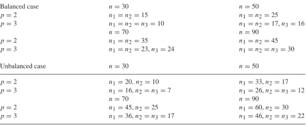
Table 1 Group sizes Balanced case n=30 n=50 p=2 n1=n2=15 n1=n2=25 p=3 n1=n2=n3=10 n1=n2=17,n3=16 n=70 n=90 p=2 n1=n2=35 n1=n2=45 p=3 n1=n2=23,n3=24 n1=n2=n3=30 Unbalanced case n=30 n=50 p=2 n1=20, n2=10 n1=33,n2=17 p=3 n1=16,n2=n3=7 n1=26,n2=n3=12 n=70 n=90 p=2 n1=45,n2=25 n1=60,n2=30 p=3 n1=36,n2=n3=17 n1=46,n2=n3=22

We have takenˆas in (9), that in this case is the minimum variance unbiased estimator ofunder the null hypothesis [1, Chapter 19]. As noted in Section 4, for our choice of G andˆ, we can assume that=0 and=I_d.

Ford =1(1)5 andn=30(20)90 we have considered a one-way ANOVA model with

p groups,p=1(i.i.d. case),2,3, and several group sizes,n_g, 1gp. For each value of

p2 and n we have studied two cases: the balanced case, where the group sizes are equal or quite similar, and the unbalanced case, where the size of one of the groups is much bigger than the rest (approximately double). The considered group sizes are displayed in Table 1.

For each value of p and n and for each case, we generated 10 000 null replications of

nVn. Tables 2–6, one for each considered dimension, display the empirical 1−percentage points of the null distribution ofnV_nbased on the above-mentioned replications. In these tables, forp2 and each value of, the cells are split into two subcells: the left subcell displays the corresponding percentage point for the balanced case, and the right subcell contains the corresponding percentage point for the unbalanced case. Looking at these tables we see that in all cases the quantiles ofnV_nfor p = 2,3 are quite close to those forp =1. The closeness is similar for both, the balanced and the unbalanced cases. As it was observed in [4,18] forp=1, we also observe rapid convergence of these quantiles to their limiting value, specially forn50, in the sense that the tabulated percentage points forn=50,70,90 are quite close for each p and quite close to the percentage points for

p=1.

5.2. Study 2: power and comparison with other tests

In Section 3 we showed that, for adequate choices of the weight function G, the test that rejectsH0for large values ofnVnis consistent. To study the ﬁnite sample performance of the proposed test and to compare it with other existing tests, we have carried out another simulation study. We have considered a one-way ANOVA model withp =3 groups,n=

(13)

Table 2

Simulated percentage points of the null distribution ofnV_nford=1

1− 0.90 0.95 0.975 0.99 0.28 0.36 0.45 0.55 p=1 n=30 0.27 0.27 0.36 0.36 0.44 0.44 0.56 0.56 p=2 0.27 0.28 0.35 0.36 0.44 0.45 0.54 0.59 p=3 0.29 0.37 0.44 0.55 p=1 n=50 0.29 0.29 0.38 0.37 0.46 0.45 0.58 0.57 p=2 0.29 0.28 0.38 0.37 0.47 0.46 0.59 0.57 p=3 0.28 0.37 0.46 0.57 p=1 n=70 0.29 0.29 0.37 0.37 0.46 0.47 0.60 0.58 p=2 0.28 0.29 0.36 0.37 0.45 0.45 0.55 0.58 p=3 0.29 0.37 0.46 0.58 p=1 n=90 0.28 0.28 0.37 0.36 0.46 0.46 0.58 0.57 p=2 0.29 0.29 0.37 0.37 0.47 0.46 0.59 0.56 p=3 Table 3

Simulated percentage points of the null distribution ofnVnford=2

1− 0.90 0.95 0.975 0.99 0.45 0.54 0.61 0.71 p=1 n=30 0.45 0.45 0.53 0.53 0.60 0.60 0.71 0.70 p=2 0.46 0.46 0.54 0.54 0.62 0.61 0.72 0.72 p=3 0.46 0.54 0.61 0.72 p=1 n=50 0.45 0.46 0.53 0.54 0.60 0.62 0.70 0.71 p=2 0.46 0.47 0.55 0.55 0.63 0.63 0.75 0.74 p=3 0.46 0.55 0.63 0.73 p=1 n=70 0.46 0.47 0.54 0.55 0.61 0.63 0.72 0.73 p=2 0.46 0.46 0.55 0.55 0.62 0.63 0.71 0.72 p=3 0.47 0.55 0.63 0.73 p=1 n=90 0.47 0.46 0.54 0.54 0.62 0.62 0.71 0.70 p=2 0.47 0.47 0.54 0.55 0.62 0.62 0.71 0.72 p=3

30(20)90, group sizes as in Table1 for the balanced case andd =1, because as we noted in the introduction, the existing tests for testingH0have been designed for univariate data. For testing the null hypothesis of univariate normality,F0=N(0,1), we have employed: the test proposed here (P), the Cramér–von Mises test (CvM) applied to the Studentized residuals, the test proposed by Bai [2](B), the test in Jiang [20] (J) and the test in Baltagi

(14)

Table 4

1− 0.90 0.95 0.975 0.99 0.60 0.66 0.71 0.79 p=1 n=30 0.58 0.58 0.65 0.64 0.71 0.70 0.78 0.79 p=2 0.58 0.60 0.65 0.66 0.70 0.74 0.78 0.83 p=3 0.60 0.66 0.72 0.80 p=1 n=50 0.60 0.60 0.67 0.66 0.73 0.72 0.81 0.78 p=2 0.60 0.60 0.66 0.67 0.72 0.74 0.80 0.82 p=3 0.61 0.67 0.73 0.81 p=1 n=70 0.60 0.61 0.67 0.67 0.73 0.73 0.81 0.81 p=2 0.60 0.61 0.67 0.68 0.73 0.73 0.81 0.82 p=3 0.61 0.68 0.74 0.82 p=1 n=90 0.61 0.61 0.67 0.67 0.73 0.73 0.80 0.81 p=2 0.61 0.61 0.67 0.68 0.73 0.74 0.81 0.82 p=3 Table 5

Simulated percentage points of the null distribution ofnVnford=4

and Li[3]. We have considered two nominal levels:=0.10, 0.05. For each sample size and for the proposed test here we have taken the corresponding critical points in Table 2 forp=1 andn=90 (we have considered them as the asymptotic critical points). For the CvM test we have taken the asymptotic critical points in Stephens [31] for testing univariate normality in the i.i.d. case, since as Pierce and Kopecky [28] have shown, the CvM test statistic has the same asymptotic null distribution as in the i.i.d. case. For the B test we

(15)

Table 6

have also taken the asymptotic critical points, that can be found in Bai[2]. To apply the test in Jiang [20] we have followed the author recommendation to choose the number of cells:[n1/5], where[x]means the largest integer x. With this rule, we have considered the following two cells for each sample size:(−∞,0]and(0,∞)(although forn = 30 this rule only gives one cell, we have also taken two cells, since with one cell the Jiang test statistic always takes the value 0). As in the simulations in Baltagi and Li [3], to calculate the test statistic proposed by these authors the smoothing parameter isa = ˆn−1/4. We have considered: the asymptotic critical points (B&L) and the bootstrap critical points (B&L∗), that have been approximated with 500 replications.

To study the power of the tests we have considered the following alternatives:

H1: F =√1

3t3, wheretr represents a t-Student distribution with r degrees of freedom.

H2: F = √1

3U(−3,3), where U(a, b) represents a uniform distribution on the interval(a, b).

H3: F = E(1)−1, where E(1) represents a negative exponential distribution with mean 1.

From the population in each hypothesis, includingH0, and for each sample size, we have generated 1000 samples. Table7 gives the relative frequency of the samples for whichH0 is rejected, that is, the simulated size (H0) and the simulated power (H1,H2,H3).

From among the considered tests, only two of them are asymptotically distribution free: the test in Bai [2] and the test in Baltagi and Li [3]. In both cases we have taken the asymptotic critical points (B, B&L). The simulation results reveal large differences between the true size and the nominal size of these tests, that is, the asymptotic null distribution does not provide an accurate approximation to the ﬁnite sample distribution of the test statistic. We also observe large differences for the J test. This prevents us from comparing their powers with the power of the other tests.

(16)

Table 7

Simulated size and power

n=30 n=50 n=70 n=90 0.10 0.05 0.10 0.05 0.10 0.05 0.10 0.05 H0 P 0.095 0.046 0.083 0.054 0.109 0.059 0.095 0.050 CvM 0.108 0.049 0.084 0.039 0.113 0.064 0.100 0.052 B 0.373 0.316 0.338 0.288 0.299 0.247 0.309 0.250 J 0.003 0.003 0.000 0.000 0.000 0.000 0.000 0.000 B&L 0.577 0.423 0.731 0.590 0.849 0.739 0.896 0.813 B&L∗ 0.106 0.050 0.094 0.040 0.121 0.062 0.113 0.061 H1 P 0.505 0.422 0.679 0.606 0.814 0.764 0.873 0.829 CvM 0.452 0.369 0.628 0.552 0.769 0.696 0.839 0.776 B 0.606 0.556 0.711 0.668 0.777 0.742 0.753 0.675 J 0.033 0.026 0.011 0.009 0.007 0.003 0.004 0.001 B&L 0.629 0.539 0.850 0.780 0.777 0.742 0.985 0.966 B&L∗ 0.249 0.186 0.396 0.332 0.563 0.458 0.642 0.556 H2 P 0.122 0.058 0.388 0.208 0.715 0.535 0.856 0.736 CvM 0.197 0.109 0.400 0.267 0.638 0.486 0.774 0.645 B 0.197 0.157 0.117 0.089 0.198 0.103 0.332 0.200 J 0.000 0.000 0.000 0.000 0.000 0.000 0.000 0.000 B&L 0.928 0.856 0.995 0.990 1.000 1.000 1.000 1.000 B&L∗ 0.525 0.379 0.787 0.655 0.903 0.826 0.954 0.912 H3 P 0.871 0.801 0.983 0.967 1.000 0.999 1.000 1.000 CvM 0.843 0.758 0.974 0.961 0.999 0.998 1.000 1.000 B 0.918 0.893 0.983 0.974 0.998 0.996 1.000 0.999 J 0.000 0.000 0.000 0.000 0.000 0.000 0.000 0.000 B&L 0.975 0.949 0.999 0.999 1.000 1.000 1.000 1.000 B&L∗ 0.769 0.663 0.960 0.929 0.996 0.993 1.000 1.000

For the rest of the tests (P, CvM, B&L∗) we see that all they are quite powerful for large n, but none of them is uniformly more powerful. Excepting for the alternativeH2when

n50, the test proposed here seems to be a bit more powerful than the CvM test for the considered alternatives. A deeper theoretical study is need in order to try to explain the observed differences in power of these tests.

6. Concludingremarks

This paper proposes a consistent test for testing if the errors in a linear model are from a speciﬁed distribution. The proposed test extends the ones in Baringhaus and Henze[4] and Fan [13]. Under some mild conditions, the asymptotic null distribution of the test statistic is that of a weighted sum of independent chi-square variates with one degree of freedom and it does not depend on the design matrix. Unlike some asymptotically distribution free test

(17)

statistics, Monte Carlo results show rapid convergence of the ﬁnite sample null distribution of the proposed test statistic to its limit. The test detects local alternatives approaching the null at the rateO(n−1/2).

The results in this paper can be extended to testing a composite null hypothesis, where the null distribution depends on a ﬁnite number of unknown parameters. In contrast to the caseF0known, the asymptotic null distribution of the corresponding test statistic de-pends on unknowns for any choice ofˆ,ˆ and G. Therefore, it has to be suitably approx-imated. We are studying this case and the obtained results will be the topic of a future paper.

7. Proofs

Proof of Proposition 2.1. We have that

Vn−(F ) =Vn,1−(F )+ Z2 R,n(t; ˆ)dG(t)+ Z2 I,n(t; ˆ)dG(t) +2 ZR,n(t; ˆ){Rn(t)+*Rn(t; ˆ)−R0(t)}dG(t) +2 ZI,n(t; ˆ){In(t)+*In(t; ˆ)−I0(t)}dG(t).

By applying the Cauchy–Schwarz inequality, to prove (3) it sufﬁces to show thatnZ_R,n2

(t; ˆ)dG(t)=o_P(1)andnZ2_I,n(t; ˆ)dG(t)=o_P(1). To prove this, we expressZ_R,n(t; ˆ) =6 k=1ZR,n,k(t; ˆ), where nZR,n,1(t; ˆ)= n j=1 sin(tε˜_j)w_jMt,˜ nZR,n,2(t; ˆ)= n j=1 sin{(y_j −x_j˜)˜−1/2t} −sin{(y_j −x_j)˜−1/2t} w_jt, nZR,n,3(t; ˆ)= n j=1 sin(ε_j1/2˜−1/2t)−sin(ε_jt) w jt, nZR,n,4(t; ˆ)= (1−) n j=1 sin(tε˜_j)w_jMt, nZR,n,5(t; ˆ)= n j=1 sin{(y_j −x_j˜)˜−1/2t} −sin{(y_j −x_j)˜−1/2t} ε_jMt, nZR,n,6(t; ˆ)= n j=1 sin(ε_j1/2˜−1/2t)−sin(ε_jt) ε_jMt,

(18)

withε˜_j =(y_j −x_j)˜ ˜−1/2,w_j =x_j(ˆ−)−1/2, 1jn,M =1/2ˆ−1/2−I_dand ˜ M=1/2˜−1/2₋_I d. From nZ2 R,n,1 n 1/4_Mt˜ 2 1 √ n n j=1w jwj , nZ2 R,n,2 t2(M˜ +Id)t2 1 √ n n j=1w jwj 2 , nZ2 R,n,3 t 2_n1/4_Mt˜ 2 1 √ n n j=1w jwj _n1 n j=1 ε jεj , nZ2 R,n,4 n1/4Mt2 1 √ n _n j=1w jwj , nZ2 R,n,5 (M˜ +Id)t 2_n1/4_Mt˜ 2 1 √ n n j=1w jwj 1_n n j=1ε jεj , nZ2 R,n,6 n1/4Mt˜ 2n1/4Mt2 1 n n j=1ε jεj 2 ,

we getn Z_R,n2 (t; ˆ)dG(t)=o_P(1). Analogously,nZ_I,n2 (t; ˆ)dG(t)=o_P(1).

Proof of Proposition 2.2. We have that

Vn,1−(F ) = Vn,2−(F )+ {*Rn(t; ˆ)−*ER(t; ˆ)}2dG(t) + {*In(t; ˆ)−*EI (t; ˆ)}2dG(t) +2 {*Rn(t; ˆ)−*ER(t; ˆ)}{Rn(t)+*ER(t; ˆ)−R0(t)}dG(t) +2 {*In(t; ˆ)−*EI (t; ˆ)}{In(t)+*EI (t; ˆ)−I0(t)}dG(t).

Applying the Cauchy–Schwarz inequality in the right-handside of the above equality, to prove (4) it sufﬁces to show that n{*R_n(t; ˆ)−*ER(t; ˆ)}2dG(t) = o_P(1) and

n{*In(t; ˆ)−*EI (t; ˆ)}2dG(t)=o_P(1). Letw₁_j=n_k₌₁h_jk (ε_k;),w₂_j=h_j.1_nn_k₌₁

hk.(εk;),w₃_j =h_j._n1n_k₌₁(ε_k;)andw₄_j =x_jB, 1jn. We have that*R_n(t; ˆ) −*ER(t; ˆ)=A1+A2+A3+A4−A5, with Ak = _n1 _n j=1 sin(tε_j)−I (t)w_kj −1/2t, 1k4, A5 = 1 n _n j=1 sin(tε_j)ε_j+ ∇R(t)(1/2ˆ−1/2−I_d)t and ∇R(t) ₌ * *t1 R(t), * *t2 R (t), . . . , * *tdR(t) .

(19)

To prove thatn{*R_n(t; ˆ)−*ER(t; ˆ)}2dG(t)=o_P(1)we will show thatnA2_kdG(t)= oP(1), 1k5.A1satisﬁes 0E n A2 1dG(t) C1hmax p n +C2 p n +C3 _p n + p2 n , whereC1–C3 are ﬁnite constants, and hence n

A2

1dG(t) = oP(1). Similarly we get

nA2

kdG(t)=oP(1),k=2,3. ForA4, we have that

n A2 4dG(t)4 n j=1 w2j2 t−1_t_d_G(t)₌_o P(1).

LetM=(m_rs)=1/2ˆ−1/2−I_d anda(ε;t)= {sin(tε)ε+ ∇R(t)}. With this notation nA2

5dG(t)can be expressed as follows

n A2 5dG(t)= d r,s,u,v=1 mrsmuv(Vrsuv,1+Vrsuv,2), where Vrsuv,1= 1 n n j=1 ar(εj;t)au(εj;t)tstvdG(t), Vrsuv,2= 1 n 1j<kn ar(εj;t)au(εk;t)+ar(εk;t)au(εj;t)tstvdG(t). By SLLN we have thatV_rsuv,1=ϑrsuv+o(1), withϑrsuv=E(Vrsuv,1) <∞, 1r, s, u,

vd, and from Theorem 5.5.2 in[30] we have that V_rsuv,2 = OP(1), 1r, s, u, vd. ThereforenA2₅dG(t)=o_P(1).

Proceeding analogously, it can be shown that n{*I_n(t; ˆ) − *EI (t; ˆ)}2dG(t) =oP(1).

Proof of Proposition 2.3. The result follows from

n  1 n n j=1 A(t)w_j−1/2_t   2 dG(t) n j=1 wj2 t−1_t_d_G(t)₌_o P(1),

withw_j =x_jB, 1jn,n{∇A(t)St}2dG(t)=o_P(1),whereA(t)=I (t)orA(t)= R(t), and the Cauchy–Schwarz inequality.

(20)

Proof of Lemma 2.1. UnderH0we have that 0E(nV_n,3)= C1+C2 1 n n j=1 h2 j.+C3h 2 .. n3 n j=1 h2 j.+C4h 2 .. n2 +C5 1 n n j=1 hj.+C6h.. n2 n j=1 hj.+C7h.. n,

whereC_k, 1k7 are ﬁnite constants. Since _n1n_j₌₁h_j.= 1_nn_j₌₁h2_j. = _n1H1n2 1

n1n2=1,by Markov inequality we getVn,3=OP(1).

Proof of Theorem 2.1. Since conditions C.3 and C.5 imply condition C.2, and C.6 implies condition C.1, the result follows from Propositions2.1–2.3 and Lemma 2.1.

Proof of Corollary 2.2. We have thatV_n,3 = _n12

_n

j,k=1K(εj, εk), whereK(x, y)is as deﬁned in (6). Since (F0) = 0, Theorem 6.4.1.B in [30] and Theorem 2.1 imply the result.

Proof of Lemma 3.1. Eq. (7) is obtained by applying elementary formulas for the sine and the cosine of a sum.

Proof of Theorem 3.1. Since|u(x)−u(y)|Cx−yand|u0(x)−u0(y)|Cx−y, for some positive ﬁnite constant C, by Lemma 3.1 we have that

|Vn−Vn,0|4C1 n n j=1 ej−εj.

Letw_kj be as in the proof of Proposition2.2, 1k4, 1jn,M =−1/2ˆ−1/2−I_d andA=(a_uv)=MM. With this notation, we have the following inequality:

ej−εj 4 k=1 −1/2_w kj + Mεj + 4 k=1 M−1/2_w kj. (12)

To show the result, we will see that_n1n_j₌₁T_j =o_P(1)for every term,T_j, in the right-hand side of (12). For the ﬁrst term in the right-hand side of (12) we have

0E    1 n n j=1 −1/2_w 1j   C1 _p n 1/2 =o(1),

(21)

whereC1 is a positive ﬁnite constant, and hence _n1

_n

j=1−1/2w1j = oP(1). Analo-gously we get1_nn_j₌₁−1/2w_kj =o_P(1),k=2,3. We also have that

1 n n j=1 −1/2_w 4j11/2(− 1₎  1 n n j=1 w4j2   1/2 =oP(n−1/2),

where1(−1)is the greatest eigenvalue of−1. For the ﬁfth term in the right-hand side of (12) we have 1 n n j=1 Mεj  1 n n j=1 ε_jAεj   1/2 =  d u,v=1 auv1_n n j=1 εjuεjv   1/2 =oP(1). Analogously we get1_nn_j₌₁M−1/2w_kj =o_P(1), 1k4.

Proof of Corollary 3.1. From Lemma3.1, we have that

Vn,0= 1 n2 n j=1 h(εj, εj)+_n12 n j=k h(εj, εk)=(F )+oP(1), (13) where the last equality follows from SLLN, Theorem 5.4.A in [30] and the fact that |h(εj, εk)|4, 1j, kn. Finally, the result follows from (13) and Theorem 3.1. Proof of Theorem 3.2. From Theorem 2.3 in [15] we have that

lim n→∞P (nVn,3x)=P    k1 k(Zk+ck)2x   . (14)

The result follows from (14) and Propositions 2.1–2.3.

Acknowledgments

The authors thank the anonymous referees and an Associate Editor for their constructive comments and suggestions which helped to improve the presentation. This research was supported in part by MEC (Spain), grant MTM2004-01433.

References

[1]S.F. Arnold, The Theory of Linear Models and Multivariate Analysis, Wiley, New York, 1981.

[2]J. Bai, Testing parametric conditional distributions of dynamic models, Rev. Econ. Statist. 85 (2003) 531–549.

(22)

[3]B.H. Baltagi, Q. Li, A consistent test for the parametric distribution of regression disturbances, Adv. Econometrics 14 (2000) 3–24.

[4]L. Baringhaus, N. Henze, A consistent test for multivariate normality based on the empirical characteristic function, Metrika 35 (1988) 339–348.

[5]P.J. Bickel, M. Rosenblatt, On some global measures of the deviations of density function estimates, Ann. Statist. 1 (1973) 1071–1095.

[6]S. Csörg˝o, Testing for normality in arbitrary dimension, Ann. Statist. 14 (1986) 708–723.

[7]M.L. Eaton, M.D. Perlman, The non-singularity of generalized sample covariance matrices, Ann. Statist. 4 (1973) 710–717.

[8]T.W. Epps, Limiting behavior of the ICF test for normality under Gram-Charlier alternatives, Statist. Probab. Lett. 42 (1999) 175–184.

[9]T.W. Epps, L.B. Pulley, A test for normality based on the empirical characteristic function, Biometrika 70 (1983) 723–726.

[10]Y. Fan, Testing the goodness-of-ﬁt of a parametric density function by kernel method, Econometric Theory 10 (1994) 316–356.

[11]Y. Fan, Bootstrapping a consistent nonparametric goodness-of-ﬁt test, Econometric Rev. 14 (1995) 367–382. [12]Y. Fan, Goodness-of-ﬁt tests for a multivariate distribution by the empirical characteristic function, J.

Multivariate Anal., doi:10.1006/jmva.1997.1672.

[13]Y. Fan, Goodness-of-ﬁt tests based on kernel density estimators with ﬁxed smoothing parameters, Econometric Theory 14 (1998) 604–621.

[14]W. Feller, An Introduction to Probability Theory and its Applications, vol. 2, Wiley, New York, 1971. [15]G.G. Gregory, Large sample theory forU-statistics and test of ﬁt, Ann. Statist. 5 (1977) 110–123. [16]P. Hall, Central limit theorem for integrated square error of multivariate nonparametric density estimators, J.

Multivariate Anal. 14 (1984) 1–16.

[17]P. Hall, A.H. Welsh, A test for normality based on the empirical characteristic function, Biometrika 70 (1983) 485–489.

[18]N. Henze, T. Wagner, A new approach to the BHEP tests for multivariate normality, J. Multivariate Anal., doi:10.1006/jmva.1997.1684.

[19]P.J. Huber, Robust regression: asymptotics, conjectures and Monte Carlo, Ann. Statist. 1 (1973) 799–821. [20]J. Jiang, Goodness-of-ﬁt tests for mixed model diagnostics, Ann. Statist. 29 (2001) 1137–1164.

[21]M.D. Jiménez-Gamero, J. Muñoz-García, M.V. Alba-Fernández, Goodness-of-ﬁt tests based on the empirical characteristic function, submitted for publication.

[22]H. Koul, Weighed Empiricals and Linear Models, IMS, Hayward, CA, 1992.

[23]I.A. Koutrouvelis, A goodness-of-ﬁt test of simple hypothesis based on the empirical characteristic function, Biometrika 67 (1980) 238–240.

[24]I.A. Koutrouvelis, J. Kellermeier, A goodness-of-ﬁt test based on the empirical characteristic function when parameters must be estimated, J. R. Statist. Soc. B 43 (1981) 173–176.

[25]E. Mammen, Asymptotics with increasing dimension for robust regression with applications to the bootstrap, Ann. Statist. 17 (1989) 382–400.

[26]E. Mammen, Empirical process of residuals for high-dimensional linear models, Ann. Statist. 24 (1996) 307–335.

[27]K. Murota, K. Takeuchi, The studentized empirical characteristic function and its application to test the shape of distribution, Biometrika 68 (1981) 55–65.

[28]D.A. Pierce, K.J. Kopecky, Testing goodness of ﬁt for the distribution of errors in regression models, Biometrika 66 (1979) 1–5.

[29]S. Portnoy, Asymptotic behaviour of the empiric distribution ofM-estimated residuals from a regression model with many parameters, Ann. Statist. 14 (1986) 1152–1170.

[30]R.J. Serﬂing, Approximation Theorems of Mathematical Statistics, Wiley, New York, 1980.

[31]M.A. Stephens, Asymptotic results for goodness-of-ﬁt statistics with unknown parameters, Ann. Statist. 4 (1976) 357–369.

[32]A.H. Welsh, A note on scale estimates based on the empirical characteristic function and their application to test for normality, Statist. Probab. Lett. 2 (1984) 345–348.