Multivariate mixtures of
Erlangs for density
estimation under censoring
Verbelen R, Antonio K, Claeskens, G.
Multivariate mixtures of Erlangs for density
estimation under censoring
Roel Verbelen∗1, Katrien Antonio1,2, and Gerda Claeskens1
1LStat, Faculty of Economics and Business, KU Leuven, Belgium.
2Faculty of Economics and Business, University of Amsterdam, The Netherlands.
August 20, 2015
Abstract
Multivariate mixtures of Erlang distributions form a versatile, yet analytically tractable, class of distributions making them suitable for multivariate density estimation. We present a flexible and effective fitting procedure for multivariate mixtures of Erlangs, which itera-tively uses the EM algorithm, by introducing a computationally efficient initialization and adjustment strategy for the shape parameter vectors. We furthermore extend the EM al-gorithm for multivariate mixtures of Erlangs to be able to deal with randomly censored and fixed truncated data. The effectiveness of the proposed algorithm is demonstrated on simulated as well as real data sets.
Keywords: Multivariate mixtures of Erlangs with a common scale parameter; Density estima-tion; Censored data; Expectation-maximization algorithm; Maximum likelihood.
1
Introduction
We present an estimation technique for fitting multivariate mixtures of Erlang distributions (MME). We suggest an efficient initialization method and adjustment strategy for the values of the shape parameter vectors of an MME, which has been underexposed in the literature. The fitting procedure is also extended to take random censoring and fixed truncation into account.
∗
The proposed algorithm has been implemented in R and is available online at www.http:// feb.kuleuven.be/roel.verbelen. Data are censored in case you only observe an interval in which a data point is lying without knowing its exact value. Truncation entails that it is only possible to observe the data of which the values lie in a certain range. Censoring and/or truncation is often the case in applications such as loss modeling (finance and actuarial science), clinical experiments (survival/failure time analysis), veterinary studies (e.g. mastitis studies), and duration data (econometric studies).
The class of MME is introduced by Lee and Lin (2012). MME form a highly flexible class of distributions as they are dense in the space of positive continuous multivariate distributions in the sense of weak convergence, extending this property of the univariate class (Tijms, 1994). An overview of the analytical and distributional properties of mixtures of Erlangs can be found in Klugman et al. (2013), Willmot and Lin (2011) and Willmot and Woo (2007). Parameter estimation in the univariate case is treated in Lee and Lin (2010) and extended to be able to deal with randomly censored and fixed truncated data in Verbelen et al. (2015).
Mixtures of Erlangs have received most attention in the field of actuarial science. Cossette et al.
(2013a) model the joint distribution of a portfolio of dependent risks using univariate mixtures of Erlangs as marginals along with the Farlie-Gumbel-Morgenstern (FGM) copula. Cossette et al. (2013b) and Mailhot (2012) study the bivariate lower and upper orthant Value-at-Risk and use MME as an illustration. Willmot and Woo (2015) study the analytical properties of the MME class. They motivate the use of MME in actuarial science and illustrate how their tractability leads to closed-form expressions.
The use of MME should be regarded as a multivariate density estimation technique, not as as a type of model-based clustering. The MME model can be seen as semiparametric, since the mixture components have a specific parametric form, whereas the mixing weights can have a nonparametric nature, and is an interesting alternative to the use of copulas, which is the dominant choice to model multivariate data in a two stage procedure, separating the dependence structure from the marginal distributions (see e.g. Joe, 1997;Nelsen,2006). In contrast, MME are able to model the multivariate data directly on the original scale. The MME model enjoys many desirable properties of a multivariate model as listed byJoe(1997, p. 84), seeLee and Lin
(2012), with regard to interpretability, closure, flexibility and wide range of dependence, and closed-form representation, often not satisfied for the commonly used copula structures.
Peel, 2001). Lee and Scott (2012) discuss the estimation of multivariate Gaussian mixtures in case the data can be randomly censored and fixed truncated. Due to the limitations of Gaussian mixtures, such as the difficulty in modeling skewed data, non-Gaussian approaches have received an increasing interest over the last years. Important examples include mixtures of multivariate t-distributions (see e.g. Peel and McLachlan, 2000), mixtures of multivariate skew-normal distributions (see e.g.Lin,2009), and mixtures of multivariate skew-t distributions (see e.g. Lee and McLachlan, 2014). All of these mixture models involve modeling real-valued multivariate random variables, whereas in this paper we consider multivariate positive-valued random variables.
Lee and Lin(2012) show in Theorem 2.3 that a finite multivariate Erlang mixture is a multivari-ate phase-type distribution, a generalization of the class of univarimultivari-ate phase-type distributions introduced by Assaf et al. (1984). Parameter estimation for phase-type distributions in the bivariate case (Eisele, 2005; Zadeh and Bilodeau, 2013), as in the univariate case (Asmussen et al.,1996;Olsson,1996), uses the expectation-maximization (EM) algorithm, first introduced by Dempster et al.(1977)
The EM algorithm forms the key to fit an MME to multivariate positive data. Taking censoring and truncation into account when calibrating data using copulas is cumbersome, especially in more than two dimensions, due to complicated forms of the likelihood (see e.g. Georges et al.,
2001) which are hard to optimize numerically. This is, as we will show, not the case for the MME class due to the EM algorithm. As opposed to the traditional way of dealing with grouped and truncated data using the EM algorithm (Dempster et al.,1977;McLachlan and Krishnan,2007, p. 66; McLachlan and Peel, 2001, p. 257; McLachlan and Jones,1988), we follow the approach of Lee and Scott (2012), as was done in the univariate setting (Verbelen et al.,2015).
We demonstrate the effectiveness of our proposed algorithm and the practical use of MME on a simulated dataset, the old faithful geyser data and a four-dimensional dataset of interval and right censored udder quarter infection times, each time highlighting one of the analytical aspects of MME.
2
Multivariate Erlang mixtures with a common scale parameter
In this section, we briefly revise the definition of a multivariate mixture of Erlang distributions with a common scale parameter and the denseness property of this distributional class. These
formulas are extended in Section 3.1and 3.2 towards censoring and truncation. The Erlang distribution is a positive continuous distribution with density function
f(x;r, θ) = x
r−1e−x/θ
θr(r−1)! forx >0, (1)
where r, a positive integer, is the shape parameter and θ > 0 the scale parameter (the inverse λ = 1/θ is called the rate parameter). The cumulative distribution function is obtained by integrating (1) by parts r times
F(x;r, θ) = 1− r−1 X n=0 e−x/θ(x/θ) n n! = γ(r, x/θ) (r−1)! , (2)
using the lower incomplete gamma function defined as γ(s, x) =R0xzs−1e−zdz.
A univariate Erlang distribution is in fact a gamma distribution of which the shape parameter is a positive integer and can therefore be seen as the distribution of a sum of i.i.d. exponential random variables. Lee and Lin(2012) define ad-variate Erlang mixture as a mixture such that each mixture component is the joint distribution of d independent Erlang distributions with a common scale parameter θ > 0. The dependence structure is captured by the combination of the positive integer shape parameters of the Erlangs in each dimension. We denote the positive integer shape parameters of the jointly independent Erlang distributions in a mixture component by the vector r= (r1, . . . , rd) and the set of all shape vectors with non-zero weight
by R. The mixture weights are denoted by α = {αr|r∈ R} and must satisfy αr > 0 and
P
r∈Rαr = 1. The density of a d-variate Erlang mixture evaluated in x = (x1, . . . , xd) with
xj >0 for j= 1, . . . , d can then be written as
f(x;α,r, θ) = X r∈R αrf(x;r, θ) = X r∈R αr d Y j=1 f(xj;rj, θ) = X r∈R αr d Y j=1 xrj−1 j e−xj/θ θrj(rj −1)!. (3)
The following property states that for any positive multivariate distribution there exists a se-quence of multivariate Erlang distributions that weakly converges to the target distribution. The proof is given in the appendix of Lee and Lin(2012).
Property 1 (Lee and Lin 2012). The class of multivariate Erlang mixtures of form (3) is dense in the space of positive continuous multivariate distributions in the sense of weak convergence.
cumulative distribution function F(x). For any given θ > 0, define the following d-variate Erlang mixture f(x;θ) = ∞ X r1=1 · · · ∞ X rd=1 αr(θ) d Y j=1 f(xj;rj, θ), (4)
with mixing weights
αr(θ) = Z r1θ (r1−1)θ · · · Z rdθ (rd−1)θ f(x)dx. (5) Then lim
θ→0F(x;θ) =F(x) for each point x at whichF is continuous.
In Property 1, for any given common scale θ > 0, an infinite multivariate mixture of Erlangs in (4) is considered using combinations of shapes from 1 to infinity in each marginal dimension. The weights in (5) of the components in the mixture are defined by integrating the density over the corresponding d-dimensional rectangle of the d-dimensional grid formed by the shape parameters multiplied with the common scale. When the value of the common scaleθdecreases, this grid becomes more refined and the sequence of Erlang mixtures converges to the underlying cumulative distribution function.
Next to its flexibility, Lee and Lin (2012) show that it is easy to work analytically with this class of distributions due to the independence structure of the Erlang distributions within each mixture component. This leads to explicit expressions of many distributional quantities such as the characteristic function, the joint moments and bivariate measures of association (Kendall’s tau and Spearman’s rho). The authors further reveal interesting closure properties, such as the fact that eachp-variate marginal or conditional distribution with p6dcan again be written as a p-variate Erlang distribution. The same property holds for the distribution of the multivari-ate excess losses (actuarial science context) or multivarimultivari-ate residual lifetimes (survival analysis context). Furthermore, the distribution of the sum of the component random variables of an MME distributed random variable is a univariate Erlang mixture distribution.
Willmot and Woo (2015) consider an extension of the MME class, allowing different scale pa-rameters in each dimension. However, in Proposition 1 they show how a multivariate mixture of Erlangs distribution with different scale parameters can be rewritten as a multivariate mixture of Erlangs distribution with a common scale parameter, which is smaller than all original scales. We thus concentrate on models with a common scale parameter.
3
Parameter estimation
The parameters of an MME to be estimated are the common scale parameter θ, the mixture weights α = {αr|r∈ R} and the set of corresponding shape parameter vectors R. Lee and
Lin (2012) propose an EM algorithm in order to find the maximum likelihood estimators for Θ= (α, θ), given a fixed set of shape parameter vectorsR. Model selection for the number of mixture components and the corresponding values of the shape parameter vectors is based on an information criterion, similar to the univariate strategy of Lee and Lin(2010) and Verbelen et al. (2015).
The two main novelties we present in this paper are (i) an extension of the EM algorithm to be able to deal with randomly censored and fixed truncated data and (ii) a computationally more efficient initialization and adjustment strategy for the shape parameter vectors in order to make the estimation procedure more flexible and effective. The improvements (i) and (ii) allow us to analyze realistic data with diverse forms of dependence in contrast to the simulated example in
Lee and Lin (2012) with a simple structure.
First we discuss how we represent a censored and truncated sample and evaluate the expression of the likelihood. The form of the complete data log-likelihood is given next, followed by the adjusted EM algorithm and a discussion on some asymptotic properties. In Section4, we present the initialization and selection of the shape parameter vectors.
3.1 Randomly censored and fixed truncated data
We represent a censored sample, truncated to the fixed range [tl,tu], byX ={(li,ui)|i= 1, . . . , n}.
The lower and upper truncation points aretl= (tl1, . . . , tld) andtu = (tu1, . . . , tud), which are com-mon to each observationi= 1, . . . , n. The lower and upper censoring points areli= (li1, . . . , lid)
andui= (ui1, . . . , uid). It holds thattl6li6ui 6tufori= 1, . . . , n. tlj = 0 andtuj =∞mean
no truncation from below and above for the jth dimension, respectively. The censoring status for the jth dimension of observation iis determined as follows:
Uncensored: tlj 6lij =uij =:xij 6tuj
Left Censored: tlj =lij < uij < tuj
Right Censored: tlj < lij < uij =tuj
Interval Censored: tlj < lij < uij < tuj.
contains the jth element of observationi. A missing value in dimension j for observationican also be dealt with by settinglij =tlj anduij =tuj, i.e. treating the missing value as a data point
being interval censored between the lower and upper truncation points.
The likelihood of a censored and truncated sample of a multivariate Erlang distribution is given by L(Θ;X) = n Y i=1 P r∈RαrQdj=1f(lij, uij;rj, θ) P(tl6Xi 6tu;Θ) with f(lij, uij;rj, θ) = f(xij;rj, θ) iflij =uij =xij F(uij;rj, θ)−F(lij;rj, θ) iflij < uij, and P(tl6Xi 6tu;Θ) = X r∈R αr d Y j=1 h F(tuj;rj, θ)−F(tlj;rj, θ) i .
The corresponding log-likelihood is
l(Θ;X) = n X i=1 ln X r∈R αr d Y j=1 f(lij, uij;rj, θ) −nln X r∈R αr d Y j=1 h F(tuj;rj, θ)−F(tlj;rj, θ) i . (6) This expression is however not workable as it involves the logarithm of a sum and cannot be used to easily find the maximum likelihood estimators for Θfor a fixed set of positive integer shape parameters R.
3.2 Construction of the complete data likelihood
For an uncensored observation xi, truncated to [tl,tu], the probability density function can be
rewritten as a mixture f(xi;tl,tu,Θ) = f(xi;Θ) P(tl6Xi6tu;Θ) = P r∈RαrQdj=1f(xij;rj, θ) P(tl6Xi6tu;Θ) =X r∈R αr·P (tl6Xi6tu;r, θ) P(tl6Xi 6tu;Θ) · Qd j=1f(xij;rj, θ) P(tl6Xi 6tu;r, θ) =X r∈R βr·f(xi;tl,tu,r, θ),
for tl 6xi 6tu and zero otherwise. The mixing weights βr and component density functions
are given by, respectively,
βr =αr·P (tl 6Xi6tu;r, θ) P(tl 6Xi6tu;Θ) =αr· Qd j=1 h F(tuj;rj, θ)−F(tlj;rj, θ) i P m∈Rαm Qd j=1 h F(tuj;mj, θ)−F(tlj;mj, θ) i (7) and f(xi;tl,tu,r, θ) = Qd j=1f(xij;rj, θ) P(tl6Xi 6tu;r, θ) = d Y j=1 f(xij;rj, θ) F(tu j;rj, θ)−F(tlj;rj, θ) . (8)
The weightsβrare re-weighted versions of the original weightsαr by means of the probabilities
of the corresponding mixture component to lie in the d-dimensional truncation interval. The component density functions f(xi;tl,tu,r, θ) are truncated versions of the original component
density functionsf(xi;r, θ).
The EM algorithm forms the solution to fit this finite mixture to the censored and truncated data. The idea is to regard the censored sample X as being incomplete since the uncensored observations xi = (xi1, . . . , xid) and their associated component-indicators zi = {zir|r∈ R}
with zir=
1 if observationxi comes from the mixture component (8)
corresponding to the shape parameter vector r
0 otherwise
(9)
for i = 1, . . . , n and r ∈ R, are not available. The complete data vector, Y = {(xi,zi)|i =
1, . . . , n}, contains all uncensored observations xi and their corresponding mixing component
indicatorzi. The log-likelihood of the complete sample Y can then be written as
l(Θ;Y) = n X i=1 X r∈R zirln βrf(xi;tl,tu,r, θ) . (10)
3.3 The EM algorithm for censored and truncated data
The EM algorithm finds the maximum likelihood estimators for Θ= (α, θ), given a fixed set
R of positive integer shape parameter vectors, based on a (possibly) censored and truncated sample by iteratively repeating the following two steps.
E-step Conditional on the incomplete dataX and using the current estimateΘ(k−1)forΘ, we compute the expectation of the complete log-likelihood (10) in thekth iteration of the E-step:
Q(Θ;Θ(k−1)) =E(l(Θ;Y)| X;Θ(k−1)) = n X i=1 E " X r∈R Zirln βrf(Xi;tl,tu,r, θ) li,ui,tl,tu;Θ(k−1) # = n X i=1 X r∈R z(irk)Ehlnβrf(Xi;tl,tu,r, θ) Zir = 1,li,ui,t l,tu;θ(k−1)i = n X i=1 X r∈R z(irk) ln(βr) + d X j=1 (rj −1)E ln(Xij) Zir= 1, lij, uij, t l j, tuj;θ(k−1) − 1 θ d X j=1 E Xij Zir = 1, lij, uij, t l j, tuj;θ(k −1)− d X j=1 rjln(θ)− d X j=1 ln((rj −1)!) − d X j=1 ln F(tuj;rj, θ)−F(tlj;rj, θ) . (11)
In the fourth equality, we apply the law of total expectation and denote the posterior probability that observation ibelongs to the mixture component corresponding to the shape parametersr
aszi(rk). These posterior probabilities can be computed using Bayes’ rule,
z(irk) =P(Zir = 1|li,ui,tl,tu;Θ(k−1)) = βr(k−1)Qdj=1 h f(lij, uij;rj, θ(k−1)) . F(tuj;rj, θ(k−1))−F(tlj;rj, θ(k−1)) i P m∈Rβ (k−1) m Qdj=1 h f(lij, uij;mj, θ(k−1)) . F(tuj;mj, θ(k−1))−F(tlj;mj, θ(k−1)) i = α (k−1) r Qdj=1f(lij, uij;rj, θ(k−1)) P m∈Rα (k−1) m Qdj=1f(lij, uij;mj, θ(k−1)) . (12)
using (7), fori= 1, . . . , nand r∈ R.
Since the terms in (11) forQ(Θ;Θ(k−1)) containingE ln(Xij) Zir= 1, lij, uij, t l j, tuj;θ(k−1) do not depend on the unknown parameter vectorΘ, they will not play a role in the EM algorithm. In the E-step, we need to compute the expected value of Xij conditional on the censoring and
truncation points and the mixing component Zir for the current valueΘ(k−1) of the parameter
vector. For i= 1, . . . , nand r∈ R, we have
E Xij Zir = 1, lij, uij, t l j, tuj;θ(k −1)
= Z uij lij x f(x;rj, θ (k−1)) F(uij;rj, θ(k−1))−F(lij;rj, θ(k−1)) dx = rjθ (k−1) F(uij;rj, θ(k−1))−F(lij;rj, θ(k−1)) Z uij lij xrje−x/θ(k−1) θ(k−1)rj+1 rj! dx = rjθ (k−1) F(u ij;rj+ 1, θ(k−1))−F(lij;rj+ 1, θ(k−1)) F(uij;rj, θ(k−1))−F(lij;rj, θ(k−1)) , (13)
in case lij < uij and in case lij =uij =xij, the observation is uncensored and the expression is
equal toxij.
M-step In thekth iteration of the M-step, we maximize the expected value (11) of the complete data log-likelihood obtained in the E-step with respect to the parameter vectorΘover all (β, θ) withβr>0,
P
r∈Rβr = 1 andθ >0. The maximization with respect to the mixing weights β,
requires the maximization of
n X i=1 X r∈R zi(rk)ln(βr),
which can be done analogously as in the univariate case, yielding
βr(k)=n−1
n
X
i=1
z(irk) forr∈ R. (14)
The average over the posterior probabilities of belonging to the jth component in the mixture forms the new estimator for the prior probability βj in the truncated mixture.
We set the first order partial derivative with respect to θ equal to zero in order to maximize Q(Θ;Θ(k−1)) over θ(see Appendix A), leading to the following M-step equation:
θ(k)= n−1Pn i=1 P r∈Rz (k) ir Pd j=1E Xij Zir = 1, lij, uij, t l j, tuj;θ(k−1) −T(k) P r∈Rβ (k) r Pdj=1rj , (15) with T(k)= X r∈R βr(k) d X j=1 tljrje−tlj/θ− tujrje−tuj/θ θrj−1(r j−1)! F(tu j;rj, θ)−F(tlj;rj, θ) θ=θ(k) .
Similar to the univariate case (Verbelen et al.,2015), the new estimatorθ(k)in (15) for the com-mon scale parameterθhas the interpretation of the expected total mean divided by the weighted total shape parameter in the mixture minus a correction termT(k)due to the truncation. Since
T(k) in (15) depends onθ(k) and has a complicated form, it is not possible to find an analytical solution. Therefore, we use a Newton-type algorithm, with the previous value of θ, i.e.θ(k−1), as starting value, to solve the equation.
We iterate the E- and M-step until the difference in log-likelihood l(Θ(k);X)−l(Θ(k−1);X) between two iterations becomes sufficiently small. By inverting expression (7), we retrieve the maximum likelihood estimator of the original mixing weightsα(rk) forr∈ R. We first compute
e αr= c βr Qd j=1 h F(tuj;rj,bθ)−F(tlj;rj,θb) i forr∈ R, (16)
where cβr and θbdenote the values in the final EM step, and then normalize the weights such
that they sum to 1.
Using the EM algorithm, the log likelihood (6) increases with each iteration (McLachlan and Krishnan,2007). The estimator for Θ= (α, θ) obtained from the EM algorithm has the same limit as the maximum likelihood estimator, whenever the starting value is adequately chosen. Hence, the maximum likelihood asymptotic theory in terms of consistency, asymptotic normality and asymptotic efficiency applies. Within the EM framework, the asymptotic covariance matrix of the maximum likelihood estimator can be assessed (McLachlan and Krishnan,2007).
These asymptotic results can only be applied with respect to Θ, given a fixed shape set R. However, the number of mixture components and the corresponding values of the shape pa-rameter vectors also have to be estimated for which we discuss a strategy in the next section. The asymptotic results stated here do not take this form of model selection into account. In Section5.3we apply a bootstrap approach to obtain bootstrap confidence intervals for the value of Kendall’s τ and Spearman’s ρ.
4
Computational details
An efficient multivariate extension of the univariate EM estimation procedure for Erlang mix-tures is not straightforward. Indeed, initialization of the parameter values and model selection are the main difficulties when estimating a multivariate Erlang mixture to a data sample and are crucial for its practical use in data analysis. We fill this gap and suggest an effective method to initialize the parameters of a multivariate Erlang mixture and a strategy to select the best set of shape parameter vectors using a model selection criterion.
4.1 Initialization and first run of the EM algorithm
Property1ensures that any positive continuous distribution can be approximated by an MME. The formulation of the property also shows how this approximation can be achieved in case the density to be approximated is available. Therefore, it serves as a starting point on how to come up with initial values in case of a sample of observations. A priori, it is however not clear how to translate the property to a finite sample setting.
Initializing data In a finite sample setting, we do not have the underlying density function at our disposal and initialize the parameters making use of an initializing data matrix y of dimension n×dwhich contains xij if the jth element of observation i is uncensored,lij in the
case of right censoring, uij in the case of left censoring, and (lij +uij)/2 in case of interval
censoring. Hence, we use popular simple imputation techniques (see e.g. Leung et al.,1997) to deal with the censoring in the initial step. If the jth element of observationiis missing or right censored at 0, we set yij equal to missing.
Shapes For any given initial common scale θ(0), instead of using an infinite set of positive integer shape parameters in each dimension (cfr. Property 1), we restrict this to a maximum numberM of shape parameters in each dimension. We select these shape parameters in a sensible way by using M quantiles ranging from the minimum to the maximum in each dimension in order to make a data-driven decision on the locations of the shape parameters. Denoting the p-percent quantile of the initializing data in dimension j by Q(p;yj), and taking into account that the expected value of a univariate Erlang distribution with shape r and scaleθ equals rθ, the set of positive integer shapes in dimension j is chosen as
{r1,j, . . . , rMj,j}= Q(p;yj) θ(0) p= 0, 1 M−1, 2 M−1, . . . ,1 . (17)
whered edenotes upwards rounding, due to the fact that the shapes have to be positive integers. Consequently, several shapes might coincide which results in Mj 6 M shape parameters in
dimension j. The initial shape set is then constructed as the Cartesian product of the dsets of positive integer shape parameters in each dimension:
Weights The shape parameters in each dimension, multiplied with the common scale param-eter θ(0), form a grid that covers the sample range. As an empirical version of Property1, the weights αr, for each shape parameter vector r = (rm1,1, . . . , rmd,d) in R, with 1 6 mj 6 Mj
for all j = 1, . . . , d, are initialized by the relative frequency of data points in thed-dimensional rectangle (rm1−1,1θ(0), rm1,1θ(0)]× · · · ×(rmd−1,dθ
(0), r
md,dθ
(0)] defined by the grid:
α(0)r=(r m1,1,...,rmd,d)=n −1 n X i=1 d Y j=1 I rmj−1,jθ (0)< y ij 6rmj,jθ (0), (19)
with r0,j = 0 for notational convenience and the indicator equal to 1/Mj in case yij is missing.
If this hyperrectangle does not contain any data points, the initial weight corresponding to the multivariate Erlang in the mixture with that shape vector will be set equal to zero. Consequently, the weight will remain zero at each subsequent iteration of the EM algorithm (see formulas (12) and (14)). Therefore, these shape vectors can immediately be removed from the set R. At initialization, the truncation is only taken into account to transform the initial values for αinto the initial values for βvia (7).
The maximal number of shape vectors is limited to Md at the initial step. However, due to the fact that Mj 6M and many shape parameter vectors will receive an initial weight equal to
zero, the actual number of shape vectors at the initial step will be lower.
Common scale The initial value of the common scaleθis the most influential for the perfor-mance of the initial multivariate Erlang mixture, as is the case in the univariate setting (Verbelen et al., 2015). A value which is too large will result in a multivariate mixture which is too flat
(‘underfit’); a value which is too small will lead to a mixture which is too peaky (‘overfit’). A
priori, it is not evident how one can make an insightful decision onθ. Similar to Verbelen et al.
(2015), we therefore introduce an additional tuning parameter: an integer spread factor s. We propose to initialize the common scale as
θ(0)= minj(maxi(yij))
Due to the use of marginal quantiles in (17) , the range of the shape parameters varies according to the sample ranges in each dimensionj = 1, . . . , dwith a maximum shape parameter equal to
rMj,j = maxi(yij) θ(0) = maxi(yij) minj(maxi(yij)) s . (21)
Hence, the spread factorsdetermines the maximum shape parameter in the dimension with the smallest maximum. The fact that the common scale parameter is equal across all dimensions is compensated by the different choice of the shape parameters in each dimension based on marginal quantiles. This ensures that the initialization works well when the ranges in each dimension are different and also gives reasonable initial approximations in case the data are skewed.
Algorithm 1 EM algorithm for a multivariate Erlang mixture.
{Initial step}
Choose M and s Compute:
θas in (20)
shape parameters in each dimension as in (17) and shape setRas in (18) mixture weights αas in (19)
R ← {r∈ R |αr6= 0}
Transform weightsα toβ as in (7)
{EM algorithm}
whilelog-likelihood (6) improvesdo
{E-step}
Compute: posterior probabilities (12) conditional expectations (13)
{M-step}
Update: weightsβ as in (14)
scaleθby numerically solving (15) end while
Transform weightsβ toα using (16) return MMEinit= (R,α,β, θ)
Apply EM algorithm Given an initial choice for the setRof shape parameter vectors, the initial common scale estimate θ(0) and the initial weights β(0) = {βr(0)|r∈ R}, we find the
maximum likelihood estimators for (β, θ) corresponding to this initial multivariate mixtures of Erlangs, denoted by MMEinit, via the EM algorithm as explained in section 3.3. An overview
4.2 Reduction of the shape vectors
The initial shape set R might not be optimal. After application of the EM algorithm, we reduce the number of mixture components of the fitted multivariate Erlang mixture. We use a backward stepwise search based on an information criterion. Information criteria, such as Akaike’s information criterion (AIC,Akaike,1974) and Schwartz’s Bayesian information criterion (BIC,Schwarz,1978), measure the quality of the model as a trade-off between the goodness-of-fit, via the log-likelihood, and the model complexity, via the number of parameters in the model. Models with a smaller value of the information criterion are preferred. Based on numerical experiments, we prefer the use of BIC over AIC since it has a stronger penalty term for the number of parameters in the model and hence leads to more parsimonious models. BIC is computed as
BIC =−2·l(Θ;X) + ln(n)· |R| ·(d+ 1), (22) where |R|indicates the number of shape parameter vectors in the shape setR.
We reduce the number of mixture components by removing all redundant shape vectors from the initial mixture based on BIC. In the backward selection strategy, depicted in pseudo code in Algorithm2, we delete the shape parameter vectorrfrom the setRfor which the corresponding mixture component has the smallest weightβr. The remaining weights are standardized to sum
to one. Along with the previous maximum likelihood estimate for the common scale, they serve as initial estimates to find the maximum likelihood estimators for (β, θ) corresponding to the reduced set Rred of shape parameter vectors by again applying the EM algorithm. In case
this maximum likelihood estimate achieves a lower BIC value, the reduced set Rred of shape parameters is accepted and we reduce the number of components further in the same manner. If not, we keep the previous set. This backward approach provides efficient initial parameter estimates for the reduced set of shape parameter vectors and ensures a fast convergence of the EM algorithm.
4.3 Adjustment of the shape vectors
In a next step we improve the shape parameter vectors of the remaining Erlang components in the mixture. Each time we adjust one of the components of a shape parameter vector by shifting its value by one (increase or decrease) and use the maximum likelihood estimates (βb,θb)
Algorithm 2 Reduction of the shape vectors inputMMEinit= (R,α,β, θ)
whileBIC (22) improvesand |R|> 1do
Rred← {r∈ R |βr 6= minr∈Rβr}
(β(0), θ(0))red←({βr/Pr∈Rredβr|r∈ Rred}, θ)
Compute MLE for (β, θ)red using the EM algorithm with initial values (β(0), θ(0))red
if BIC (22) improvesthen
R ← Rred
(β, θ)←(β, θ)red
end if end while
return MMEred= (R,α,β, θ)
of Erlang distributions with slightly adjusted shape parameter vector set Radj. These initial values are close to the maximum likelihood estimates which guarantees fast convergence. In case the maximum likelihood estimate corresponding to the adjusted set Radj achieves a lower log-likelihood value (6), the adjusted set Radj is accepted and we continue adjusting the value of the shape parameter in the same direction. If not, we keep the previous set of shape parameter combinations.
The gradual adjustment strategy of the shape parameter combinations is described in detail in Algorithm 3. While the log-likelihood improves, we continue to consecutively increase or decrease the value of a component of a shape parameter vector if it leads to a better fit. The algorithm converges when no single addition or subtraction of the value of any of the components of any of the shape parameter vectors leads to an improvement in the log-likelihood.
After adjusting the shape parameters, we apply the reduction step in combination with the adjustment step. Based on BIC we further reduce the number of shape parameter vectors by deleting the shape vector with the smallest mixture weight and adjusting the values of the remaining ones. The outline of this adjustment and further reduction of the shape parameter vectors, which results in the final MME, is given in Algorithm 4.
Algorithm 3 Adjustment of the shape combinations inputMMEred= (R,α,β, θ)
whilelog-likelihood (6) improvesdo forj ∈ {1, . . . , d} do
for re∈ R do repeat
if (er1, . . . ,erj+ 1, . . . ,erd)∈ R/ then
Radj ← {r∈ R |r6=re} ∪ {(re1, . . . ,rej+ 1, . . . ,erd)}
Compute MLE for (β, θ)adj using the EM algorithm with initial values (β, θ)
if log-likelihood (6) improves then
R ← Radj
(β, θ)←(β, θ)adj
end if end if
until(er1, . . . ,erj+ 1, . . . ,erd)∈ Ror log-likelihood (6) no longer improves end for
for re∈ R do repeat
if (er1, . . . ,erj−1, . . . ,red)∈ R/ and erj−1>1then
Radj ← {r∈ R |r6=re} ∪ {(re1, . . . ,rej−1, . . . ,erd)}
Compute MLE for (β, θ)adj using the EM algorithm with initial values (β, θ)
if log-likelihood (6) improves then
R ← Radj
(β, θ)←(β, θ)adj
end if end if
until(er1, . . . ,erj−1, . . . ,red)∈ Rorerj−1 = 0 orlog-likelihood (6) no longer improves end for
end for end while
return MMEadj = (R,α,β, θ)
Algorithm 4 Adjustment and further reduction of the shape vectors inputMMEadj = (R,α,β, θ)
whileBIC (22) improvesand |R|> 1do
Rred← {r∈ R |βr 6= minr∈Rβr}
(β(0), θ(0))red←({βr/Pr∈Rredβr|r∈ Rred}, θ)
Compute MLE for (β, θ)red using the EM algorithm with initial values (β(0), θ(0))red
Apply adjustment algorithm3
if BIC (22) improvesthen
R ← Radj
(β, θ)←(β, θ)adj
end if end while
5
Examples
We demonstrate the proposed fitting procedure on three datasets, each time highlighting a dif-ferent aspect of multivariate mixtures of Erlangs. In a first simulated two-dimensional example, we explicitly illustrate the different steps of the estimation procedure. Second, we model the waiting time between eruptions and the duration of the eruptions of the old faithful geyser dataset. Based on the fitted two-dimensional MME, we immediately obtain the distribution of the sum of the waiting time and the duration, representing the total cycle time. In the third example, we use multivariate mixtures of Erlangs to model the udder infection times of dairy cows observed in a mastitis study, and use the fitted MME to analytically quantify the posi-tive correlation between the udder infection times using the explicit expression of the bivariate measures of association Kendall’s tau and Spearman’s rho in the MME setting.
The resulting MME after applying the different steps in choosing the shape vectors depends heavily on the starting values. Therefore it is crucial to sufficiently explore the effect of changing the value of the tuning parameters M and sand compare the results of several different initial starting points for the shape set. In addition to the value of BIC, graphs aid the assessment of the fitted model.
5.1 Simulated data
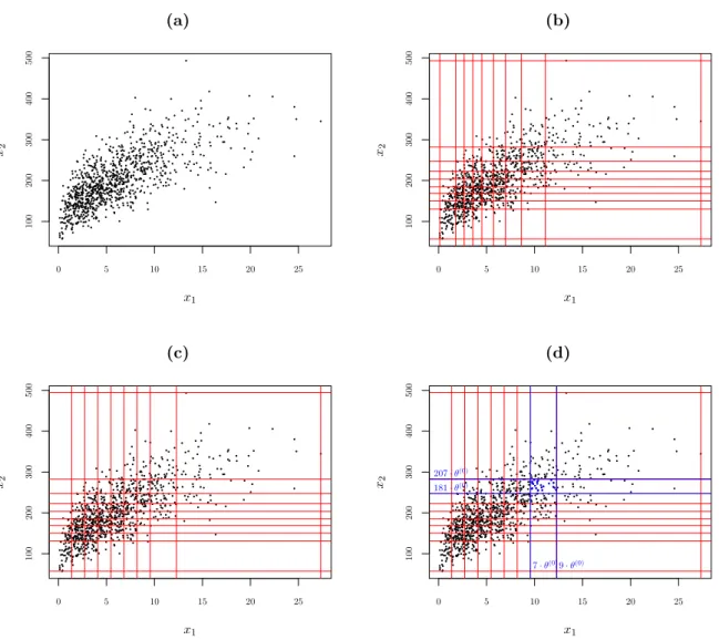
As a first example, we generate 1000 uncensored and untruncated observations from a bivari-ate normal copula with correlation coefficient 0.75 and Erlang distributed margins with shape parameter equal to 2 and 10, respectively, and scale parameter equal to 3 and 20, resp. A scatterplot of this simulated dataset is shown in Figure 1a. Due to the parameter choice, the ranges in each dimension are quite different.
We now apply the different steps of the estimation procedure on this dataset and graphically illustrate the interpretations and effects of these steps. First we consider the initialization strategy for the shape set R, the scale parameter θ and the mixture weights β, based on the denseness property of MME in Property1, as explained in Section4.1. This strategy is controlled by two tuning parameters, a maximum number M of shape parameters in each dimension and a spread factors. In this illustration, we useM = 10 ands= 20. For this choice, the scale θ is initialized as
θ(0)= minj(maxi(xij))
s =
27.32452
(a) 0 5 10 15 20 25 100 200 300 400 500 x1 x2 (b) 0 5 10 15 20 25 100 200 300 400 500 x1 x2 (c) 0 5 10 15 20 25 100 200 300 400 500 x1 x2 (d) 0 5 10 15 20 25 100 200 300 400 500 x1 x2 9·θ(0) 207·θ(0) 7·θ(0) 181·θ(0)
Figure 1: Simulated example: (a) scatterplot, (b) marginal quantile grid, (c) grid formed by multiplying the shapes (17) by the common scale (20) and (d) initial weightα(0)r=(9,207)= 0.024.
In order to make a data driven choice for the initial positions of the shape parameters, we compute M marginal quantiles in each dimension, which are depicted in Figure 1b and form a grid that covers the data range. These marginal quantiles are then divided by the initial scale θ(0) and rounded upwards to initialize the shape parameters in each dimension:
{r1,j, . . . , rMj,j}= Q(p;xj) θ(0) p= 0,1 9, 2 9, . . . ,1 forj= 1,2.
dimension:
R={r1,1, . . . , rM1,1} × {r1,2, . . . , rM2,2}
={1,2,3,4,5,6,7,9,20} × {42,96,110,124,136,149,163,181,207,362}.
Due to the rounding, shape 2 appears twice in the first dimension and only 9 instead of 10 shapes remain in that dimension. Due to the choice of θ(0), s= 20 is the maximal shape parameter in the first dimension, the dimension with the smallest maximum. The maximal shape in the second dimension is stimes the ratio of the maximum in the second dimension and the lowest maximum, rounded upwards (see (21)). If we multiply this shape set R with the initial scale θ(0), we obtain a grid that covers the entire sample range which is depicted in Figure 1c. This grid differs from the marginal quantile grid due to the rounding and is used to initialize the weights as the relative frequency of data points in the 2-dimensional rectangle corresponding to each shape vector:
α(0)r=(r m1,1,rm2,2)= 0.001 1000 X i=1 2 Y j=1 I rmj−1,jθ (0)< y ij 6rmj,jθ (0).
For example, for the shape vector r = (rm1,1, rm2,2) = (9,207), we consider the 2-dimensional
rectangle (rm1−1,1θ(0), rm1,1θ(0)]×(rm2−1,2θ(0), rm2,2θ(0)] = (7·θ(0),9·θ(0)]×(181·θ(0),207·θ(0)]
shown in Figure 1d, leading to an initial weight of
α(0)r=(9,207) = 0.001 1000 X i=1 I 7·θ(0) < yi1 69·θ(0) I 181·θ(0) < yi2 6207·θ(0) = 0.024,
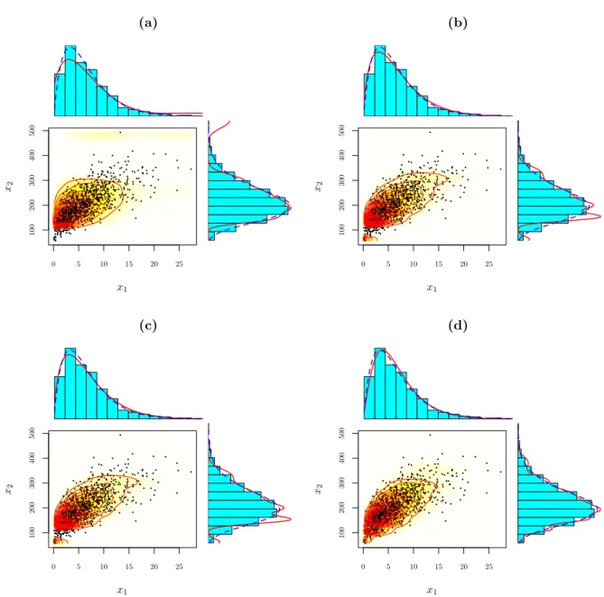
since 24 of the 1000 observations lie in this rectangle. The resulting initial MME contains 71 shape vectors with a nonzero weight and already forms a reasonable approximation for the main portion of the data. In Figure 2a, we show the scatterplot of the data with an overlay of the density of the initial MME using a contour plot and heat map. In the margins, we plot the marginal histograms with an overlay of the true densities in blue and the fitted densities in red. In the second dimension, there is too much weight in the tail and too little near the origin. After applying the EM algorithm a first time with these initial estimates, we obtain the maximum likelihood estimates of the weights and scale corresponding to this choice of the shape set (Section 4). In Figure 2b, we observe that the fit is better in the tail, but there is still too
little weight in the second dimension near the origin, due to a bad positioning of the first shape in second dimension.
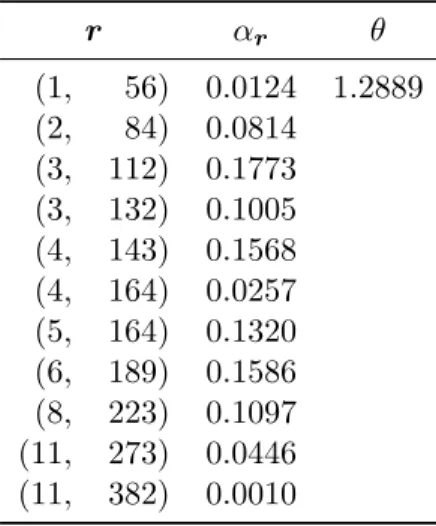
Table 1: Parameter estimates of the MME with 11 mixture components fitted to the simulated data.
r αr θ (1, 56) 0.0124 1.2889 (2, 84) 0.0814 (3, 112) 0.1773 (3, 132) 0.1005 (4, 143) 0.1568 (4, 164) 0.0257 (5, 164) 0.1320 (6, 189) 0.1586 (8, 223) 0.1097 (11, 273) 0.0446 (11, 382) 0.0010
Hence, the initial set of shape parameter vectors is not ideal and additional steps are required to improve the shape set. First, we reduce the number of mixture components from 71 to 17 by subsequently removing the mixture component having the smallest weight if it is found to be redundant based on BIC (Section 4.2). The fit of this reduced mixture in Figure 2c nearly coincides with the one in Figure 2b. Second, we adjust the values of the shape parameter vectors and further reduce the number of mixture components based on BIC (Section4.3) until we obtain a close-fitting MME with 11 shape parameter vectors (Figure 2d). The parameter estimates of this final MME are given in Table 1.
5.2 Old faithful geyser data
We consider the waiting time between eruptions and the duration of the eruption for the Old faithful geyser in Yellowstone National Park, Wyoming, USA. We use the version of Azzalini and Bowman (1990) which contains 299 observations. This dataset is popular in the field of nonparametric density estimation (see e.g.Silverman,1986;H¨ardle,1991). We stress that we use MME as a multivariate density estimation technique, and not as a mixture modeling technique to identify subgroups in this data.
We fit a two-dimensional MME to the data using the fitting strategy explained in Section4. We perform a grid search to identify good values for the tuning parametersM and s. We letsvary between 10 and 90 by 10 and between 100 and 1000 by 100 and set M equal to 5, 10 and 20.
(a) 0 5 10 15 20 25 100 200 300 400 500 x1 x2 (b) 0 5 10 15 20 25 100 200 300 400 500 x1 x2 (c) 0 5 10 15 20 25 100 200 300 400 500 x1 x2 (d) 0 5 10 15 20 25 100 200 300 400 500 x1 x2
Figure 2: Scatterplot of the simulated data with an overlay of the fitted density of the MME using a contour plot and heat map. In the margins, we plot the marginal histograms with an overlay of the true densities in blue and the fitted densities in red. In (a), we display the fit after initialization, in (b) after applying the EM algorithm a first time, in (c) after applying the reduction step and in (d) after applying the adjustment and further reduction step.
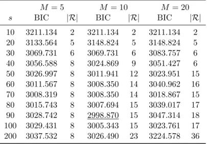
To illustrate the importance and effect of the tuning parameters, we report part of the results of the search grid, up to s= 200, in Figure 3 and Table 2. Values ofs beyond 200 resulted in MME which were overfitting the data.
Table 2: BIC values and number of mixture components when fitting an MME to the Old Faithful geyser data, starting from different values of the tuning parameters. The minimum BIC value is underlined and obtained forM = 10 ands= 90.
M = 5 M = 10 M = 20
s BIC |R| BIC |R| BIC |R|
10 3211.134 2 3211.134 2 3211.134 2 20 3133.564 5 3148.824 5 3148.824 5 30 3069.731 6 3069.731 6 3083.757 6 40 3056.588 8 3024.869 9 3051.427 6 50 3026.997 8 3011.941 12 3023.951 15 60 3011.567 8 3008.350 14 3040.962 16 70 3008.319 8 3008.350 14 3018.867 15 80 3015.743 8 3007.694 15 3039.017 17 90 3028.742 8 2998.870 15 3047.314 18 100 3029.431 8 3005.343 15 3023.761 17 200 3037.532 8 3026.490 23 3224.578 36
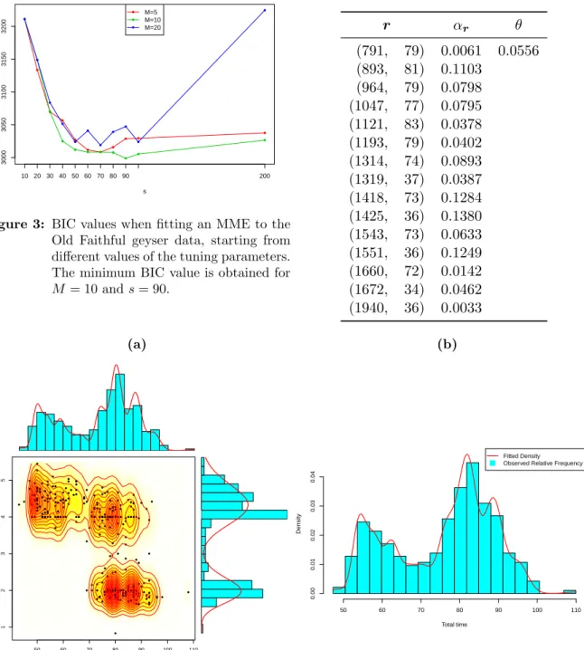
The resulting MME depends on the value of the tuning parameters. However, multiple MME can result in a satisfactory fit of the data. BIC indicates that the best-fitting MME is obtained for M = 10 ands= 90. The parameter estimates of this MME are reported in Table 3. Both the marginals as well as the dependence structure are adequately represented by this MME as is confirmed graphically in Figure 4a. Since the maximum of the waiting times is about 20 times as big as the maximum of the duration times whereas the scale parameter of the MME is the same across dimensions, the fitted marginal density is more capricious in the dimension of the waiting times and smoother in the dimension of the duration times.
We are interested in the distribution of the duration of the total cycle, i.e. the sum of the waiting time until the eruption and the duration of the eruption. Based on the fitted two-dimensional MME and due to the analytical properties of MME, we immediately obtain the distribution of this sum, which is a univariate mixture of Erlang distributions with the same scale, the sum of the shape parameters across the dimensions as shape parameters and the same corresponding weights in (Lee and Lin,2012, Theorem 5.1). Hence, the parameters of this univariate mixture of Erlang distributions are readily available from Table 3. Comparing the histogram of the observed total times to the fitted density in Figure 4breveals a close approximation.
3000 3050 3100 3150 3200 s BIC 10 20 30 40 50 60 70 80 90 200 ● ● ● ● ● ● ● ● ● ● ● ● ● ● ● ● ● ● ● ● ● ● ● ● ● ● ● ● ● ● ● ● ● ● ● ● M=5 M=10 M=20
Figure 3: BIC values when fitting an MME to the Old Faithful geyser data, starting from different values of the tuning parameters. The minimum BIC value is obtained for
M = 10 ands= 90.
Table 3: Parameter estimates of the best-fitting MME with 15 mixture components fitted to the Old Faithful geyser data.
r αr θ (791, 79) 0.0061 0.0556 (893, 81) 0.1103 (964, 79) 0.0798 (1047, 77) 0.0795 (1121, 83) 0.0378 (1193, 79) 0.0402 (1314, 74) 0.0893 (1319, 37) 0.0387 (1418, 73) 0.1284 (1425, 36) 0.1380 (1543, 73) 0.0633 (1551, 36) 0.1249 (1660, 72) 0.0142 (1672, 34) 0.0462 (1940, 36) 0.0033 (a) ● ● ● ● ● ● ● ● ● ● ● ● ● ● ● ● ● ● ● ● ● ● ● ● ● ● ● ● ● ● ● ● ● ● ● ● ● ● ● ● ● ● ● ● ● ● ● ● ● ● ● ● ● ● ● ● ● ● ● ● ● ● ● ● ● ● ● ● ● ● ● ● ● ● ● ● ● ● ● ● ● ● ● ● ● ● ● ● ● ● ● ● ● ● ● ● ● ● ● ● ● ● ● ● ● ● ● ● ● ● ● ● ● ● ● ● ● ● ● ● ● ● ● ● ● ● ● ● ● ● ● ● ● ● ● ● ● ● ● ● ● ● ● ●● ● ● ● ● ● ● ● ● ● ● ● ● ● ● ● ● ● ● ● ● ● ● ● ● ● ● ● ● ● ● ● ● ● ● ● ● ● ● ● ● ● ● ● ● ● ● ● ● ● ● ● ● ● ● ● ● ● ● ● ● ● ● ● ● ● ● ● ● ● ● ● ● ● ● ● ● ● ● ● ● ● ● ● ● ● ● ● ● ● ● ● ● ● ● ● ● ● ● ● ● ● ● ● ● ● ● ● ● ● ● ● ● ● ● ● ● ● ● ● ● ● ● ● ● ● ● ● ● ● ● ● ● ● ● ● ● ● ● ● ● ● ● ● ● ● ● ● ● ● ● ● ● ● ● 50 60 70 80 90 100 110 1 2 3 4 5 Waiting time Dur ation time ● ● ● ● ● ● ● ● ● ● ● ● ● ● ● ● ● ● ● ● ● ● ● ● ● ● ● ● ● ● ● ● ● ● ● ● ● ● ● ● ● ● ● ● ● ● ● ● ● ● ● ● ● ● ● ● ● ● ● ● ● ● ● ● ● ● ● ● ● ● ● ● ● ● ● ● ● ● ● ● ● ● ● ● ● ● ● ● ● ● ● ● ● ● ● ● ● ● ● ● ● ● ● ● ● ● ● ● ● ● ● ● ● ● ● ● ● ● ● ● ● ● ● ● ● ● ● ● ● ● ● ● ● ● ● ● ● ● ● ● ● ● ● ●● ● ● ● ● ● ● ● ● ● ● ● ● ● ● ● ● ● ● ● ● ● ● ● ● ● ● ● ● ● ● ● ● ● ● ● ● ● ● ● ● ● ● ● ● ● ● ● ● ● ● ● ● ● ● ● ● ● ● ● ● ● ● ● ● ● ● ● ● ● ● ● ● ● ● ● ● ● ● ● ● ● ● ● ● ● ● ● ● ● ● ● ● ● ● ● ● ● ● ● ● ● ● ● ● ● ● ● ● ● ● ● ● ● ● ● ● ● ● ● ● ● ● ● ● ● ● ● ● ● ● ● ● ● ● ● ● ● ● ● ● ● ● ● ● ● ● ● ● ● ● ● ● ● ● (b) Total time Density 50 60 70 80 90 100 110 0.00 0.01 0.02 0.03 0.04 Fitted Density Observed Relative Frequency
Figure 4: Graphical evaluation of the best-fitting MME to the Old Faithful geyser data. In (a), we display the scatterplot of the data with an overlay of the fitted density using a contour plot and heat map. The margins show the marginal histograms with an overlay of the fitted densities in red. In (b), we compare the fitted density of the sum of the components and the histogram of the observed total cycle times.
5.3 Mastitis study
Mastitis is economically one of the most important diseases in the dairy sector since it leads to reduced milk yield and milk quality. In this example, we consider infectious disease data from a mastitis study by Laevens et al. (1997). This dataset has also been used in Goethals et al.
(2009) and Ampe et al.(2012).
We focus on the infection times of individual cow udder quarters with a bacterium. As each udder quarter is separated from the three other quarters, one quarter might be infected while the other quarters remain infection-free. However, the dependence must be modeled since the data are hierarchical, with individual observations at the udder quarter level being correlated within the cow. Additionally, the infection times are not known exactly due to a period follow-up, which is often the case in observational studies since a daily checkup would not be feasible. Roughly each month, the udder quarters are sampled and the infection status is assessed, from the time of parturition, at which the cow was included in the cohort and assumed to be infection-free, until the end of the lactation period. This generates interval-censored data since for udder quarters that experience an event it is only known that the udder quarter got infected between the last visit at which it was infection-free and the first visit at which it was infected. Observations can also be right censored if no infection occurred before the end of the lactation period, which is roughly 300-350 days but different for every cow, before the end of the study or if the cow is lost to follow-up during the study, for example due to culling.
The data we consider contains information on 100 dairy cows on the time to infection of the four udder quarters by different types of bacteria. This dataset is used inGoethals et al.(2009), who model the data using an extended shared gamma frailty model that is able to handle the interval censoring and clustering simultaneously. We treat the infection times at the udder quarter level of the cow as four-dimensional interval and right censored data of which we estimate the underlying density using MME. The udder quarters are denoted as RL (rear left), FL (front left), RR (rear right) and FR (front right).
In search for the best values of the tuning parameters in the MME estimation procedure, we first fixed M = 20 and let s vary between 10 and 100 by 10 and between 100 and 1000 by 100. As the best final fit was obtained fors= 10, we variedM between 10 and 100 by 10 for sfixed at 10. The resulting fits did, however, not depend onM whensis as low as 10 since the starting values were identical. Varyingsfrom 5 tot 15 forM = 20 confirmed that the best fit is obtained
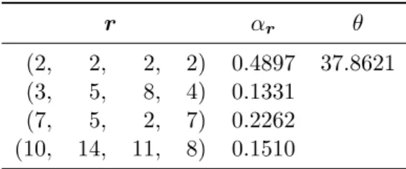
forM = 20 ands= 10. For this setting, the initial number of shape vectors was 73, which got reduced to 6 after the reduction step and to 4 after the adjustment step. The final parameter estimates of the best-fitting mixture are given in Table 4.
Table 4: Parameter estimates of the best-fitting MME with four mixture components fitted to the mastitis data (infections by all bacteria).
r αr θ
(2, 2, 2, 2) 0.4897 37.8621 (3, 5, 8, 4) 0.1331
(7, 5, 2, 7) 0.2262 (10, 14, 11, 8) 0.1510
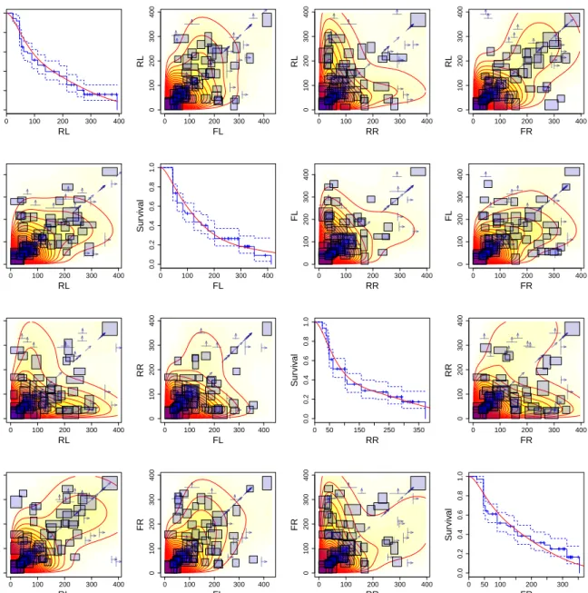
In order to graphically examine the goodness-of-fit of the fitted MME, we construct in Figure
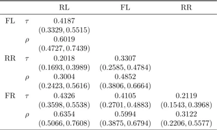
5 a generalization of the scatterplot matrix. On the diagonal we compare the Turnbull non-parametric estimate of the survival curve for right and interval censored data (Turnbull,1976), along with the log-transformed equal precision simultaneous confidence intervals (Nair,1984), to the univariate marginal survival function of the fitted MME. On the off-diagonal, we construct bivariate scatterplots of interval and right censored data points, represented using the effective visualization of Li et al.(2015). Interval censored observation are depicted as segments or rect-angles ranging from the lower to the upper censoring points and right censored observations are depicted as arrows starting from the lower censoring point and pointing to the censoring direc-tion. On top, we display the contour plot and heat map representing the density of the bivarite marginal of the fitted MME. Based on this graph, we observe that in four dimensions, with 100 interval and right censored observations, we are able to fit an MME with four shape parameter vectors which appropriately captures the marginals as well as the dependence structure. As a measure of the infectivity of the agent causing the disease, we are interested in the corre-lation between udder infection times. Due to the fact that the bivariate marginals again belong to the MME class and the analytical qualities of MME, we have closed-form expressions for Kendall’s τ and Spearman’s ρ (Lee and Lin, 2012, Theorem 3.2 and 3.3). Note that these do not depend on the common scale parameter. For the interval and right censored sample, we can hence estimate these measures based on the fitted MME to analytically quantify the positive correlation between each pair of udder quarter infection times (Table 5).
Inference is not straightforward due to the model selection as pointed out in Section3.3. In order to quantify the uncertainty and construct an approximate confidence interval for the bivariate
0 100 200 300 400 0.0 0.2 0.4 0.6 0.8 1.0 RL Sur viv al 0 100 200 300 400 0 100 200 300 400 RL FL FL missing RL missing 0 100 200 300 400 0 100 200 300 400 RL RR RR missing RL missing 0 100 200 300 400 0 100 200 300 400 RL FR FR missing RL missing 0 100 200 300 400 0 100 200 300 400 FL RL RL missing FL missing 0 100 200 300 400 0.0 0.2 0.4 0.6 0.8 1.0 FL Sur viv al 0 100 200 300 400 0 100 200 300 400 FL RR RR missing FL missing 0 100 200 300 400 0 100 200 300 400 FL FR FR missing FL missing 0 100 200 300 400 0 100 200 300 400 RR RL RL missing RR missing 0 100 200 300 400 0 100 200 300 400 RR FL FL missing RR missing 0 50 150 250 350 0.0 0.2 0.4 0.6 0.8 1.0 RR Sur viv al 0 100 200 300 400 0 100 200 300 400 RR FR FR missing RR missing 0 100 200 300 400 0 100 200 300 400 FR RL RL missing FR missing 0 100 200 300 400 0 100 200 300 400 FR FL FL missing FR missing 0 100 200 300 400 0 100 200 300 400 FR RR RR missing FR missing 0 50 100 200 300 0.0 0.2 0.4 0.6 0.8 1.0 FR Sur viv al
Figure 5: Scatterplot matrix comparing the fitted four-dimensional MME to the observed interval and right censored observations of the mastitis data (infections by all bacteria). For more expla-nation, see Section5.3
measures of association, we resort to a bootstrapping procedure (Efron and Tibshirani, 1994). By sampling with replacement from the original four-dimensional dataset of size 100, we generate 1000 bootstrap samples of the same size 100. For each of these bootstrap samples, we fit an MME where we set the tuning parameter M equal to 20 and let s vary between 5 and 25. We choose this fixed grid for each bootstrap sample since the optimal tuning parameters for the full sample wereM = 20 and s= 10 and the starting values are not that sensitive with respect
to M for low values of s. We thereby obtain 1000 estimates for each measure of association. The 5% and 95% quantiles of these estimates are used to construct a 90% bootstrap percentile confidence interval for each Kendall’sτ and Spearman’sρ in Table5.
Table 5: Estimates and 90% bootstrap confidence intervals for the bivariate measures of association Kendall’sτ and Spearman’sρbased on the fitted MME for the mastitis data (infections by all bacteria). RL FL RR FL τ 0.4187 (0.3329,0.5515) ρ 0.6019 (0.4727,0.7439) RR τ 0.2018 0.3307 (0.1693,0.3989) (0.2585,0.4784) ρ 0.3004 0.4852 (0.2423,0.5616) (0.3806,0.6664) FR τ 0.4326 0.4105 0.2119 (0.3598,0.5538) (0.2701,0.4883) (0.1543,0.3968) ρ 0.6354 0.5994 0.3122 (0.5066,0.7608) (0.3875,0.6794) (0.2206,0.5577)
6
Discussion
MME form a highly flexible class of distributions which are at the same time mathematically tractable. From Property1, we know that any positive continuous multivariate distribution can be approximated up to any accuracy by an infinite multivariate mixture of Erlang distributions. Our contribution presents a computationally efficient initialization and adjustment strategy for the shape parameter vectors, translating this theoretical aspect in a strong point in practice as well. In the examples, we demonstrate how the fitting procedure is able to estimate an MME that adequately represents both the marginals and the dependence structure. By extending the EM algorithm, we are now also able to deal with left, interval or right censored and truncated data. MME therefore form a valuable multivariate density estimation technique to analyze realistic data, even in incomplete data settings, and to model the dependence directly in a low dimensional setting.
Their tractability allows to derive explicit expression of properties of interest. Willmot and Woo(2015) have paved the way for applying MME in insurance loss modeling, survival analysis and ruin theory. When modeling insurance losses or dependent risks from different portfolios
or lines of buniness using MME, the aggregate and excess losses have again a univariate and multivariate mixture of Erlangs distribution. Stop-loss moments, several types of premiums, risk capital allocation based on the Tail-Value-at-Risk (TVaR) or covariance rule for regulatory risk capital requirements (see e.g. Dhaene et al.,2012) have analytical expressions. When modeling bivariate lifetimes and pricing joint-life and last-survivor insurance (see e.g. Frees et al., 1996) using MME, the distribution of the minimum and maximum is again a univariate mixture of Erlangs. Such kind of data are always left truncated and right censored. The extension of the fitting procedure for MME presented in this paper, allows to take the right censoring into account. Left truncation can only be properly handled when the left truncation points are fixed for each observation. This is however not the case when pricing joint-life and last-survivor insurance since the ages at which policyholders enter a contract vary.
The reduction and adjustment steps of the shape parameters in the fitting procedure iteratively make use of the EM algorithm and can be time consuming. Further adjustment is needed to estimate parameters in high dimensional settings. As also acknowledged in the univariate case (Verbelen et al., 2015), the modeling of heavy-tailed distributions using MME is challenging since MME are not able to extrapolate the heaviness in the tail.
Acknowledgements
The authors wish to thank Dr. H. Laevens (Catholic University College Sint-Lieven, Sint-Niklaas, Belgium), for permission to use the mastitis data, and the referees for their comments. This work was supported by the agency for Innovation by Science and Technology IWT, IAP Re-search Network P6/03 of the Belgian State (Belgian ReRe-search Policy) and by KU Leuven grant GOA/12/14.
Appendix A
Partial derivative of
Q
In order to maximizeQ(Θ;Θ(k−1)) with respect toθ, we set the first order partial derivative at θ(k) equal to zero. In the second equation, expression (2) of the cumulative distribution of an
∂Q(Θ;Θ(k−1)) ∂θ θ=θ(k) = n X i=1 X r∈R zi(rk) Pd j=1E Xij Zir= 1, lij, uij, t l j, tuj;θ(k −1) θ2 − Pd j=1rj θ − d X j=1 ∂ ∂θ h F(tuj;rj, θ)−F(tlj;rj, θ) i F(tuj;rj, θ)−F(tlj;rj, θ) θ=θ(k) = 1 θ2 n X i=1 X r∈R zi(rk) d X j=1 E Xij Zir= 1, lij, uij, t l j, tuj;θ(k −1)−n θ X r∈R Pn i=1z (k) ir n ! d X j=1 rj − n X i=1 X r∈R z(irk) d X j=1 ∂ ∂θ γ(rj, tuj/θ)−γ(rj, tlj/θ) (rj −1)! F(tuj;rj, θ)−F(tlj;rj, θ) θ=θ(k) = 1 θ2 n X i=1 X r∈R zi(rk) d X j=1 E Xij Zir= 1, lij, uij, t l j, tuj;θ(k −1)−n θ X r∈R βr(k) d X j=1 rj −n θ2 X r∈R βr(k) d X j=1 tljrje−tlj/θ− tujrje−tuj/θ θrj−1(r j −1)! F(tu j;rj, θ)−F(tlj;rj, θ) θ=θ(k) = 0,
where we used expression (2) of the cumulative distribution of an Erlang in the second equality and (14) in the third.
References
Akaike, H. (1974). A new look at the statistical model identification. IEEE Transactions on
Automatic Control, 19(6):716–723.
Ampe, B., Goethals, K., Laevens, H., and Duchateau, L. (2012). Investigating clustering in interval-censored udder quarter infection times in dairy cows using a gamma frailty model.
Preventive veterinary medicine, 106(3):251–257.
Asmussen, S., Nerman, O., and Olsson, M. (1996). Fitting phase-type distributions via the EM algorithm. Scandinavian Journal of Statistics, pages 419–441.
Assaf, D., Langberg, N. A., Savits, T. H., and Shaked, M. (1984). Multivariate phase-type distributions. Operations Research, 32(3):688–702.
Azzalini, A. and Bowman, A. (1990). A look at some data on the old faithful geyser. Applied
Statistics, pages 357–365.
Cossette, H., Cˆot´e, M.-P., Marceau, E., and Moutanabbir, K. (2013a). Multivariate distribution defined with Farlie–Gumbel–Morgenstern copula and mixed Erlang marginals: Aggregation and capital allocation. Insurance: Mathematics and Economics, 52(3):560–572.
Cossette, H., Mailhot, M., Marceau, E., and Mesfioui, M. (2013b). Bivariate lower and upper orthant Value-at-Risk. European Actuarial Journal, 3(2):321–357.
Dempster, A. P., Laird, N. M., and Rubin, D. B. (1977). Maximum likelihood from incomplete data via the EM algorithm.Journal of the Royal Statistical Society. Series B (Methodological), 39(1):1–38.
Dhaene, J., Tsanakas, A., Valdez, E. A., and Vanduffel, S. (2012). Optimal capital allocation principles. Journal of Risk and Insurance, 79(1):1–28.
Efron, B. and Tibshirani, R. (1994). An Introduction to the Bootstrap. Chapman & Hall/CRC Monographs on Statistics & Applied Probability. Taylor & Francis.
Eisele, K.-T. (2005). EM algorithm for bivariate phase distributions. In ASTIN Colloquium,
Zurich, Switzerland. http://www. actuaries. org/ASTIN/Colloquia/Zurich/Eisele. pdf.
Frees, E. W., Carriere, J., and Valdez, E. (1996). Annuity valuation with dependent mortality.
Journal of Risk and Insurance, pages 229–261.
Georges, P., Lamy, A.-G., Nicolas, E., Quibel, G., and Roncalli, T. (2001). Multivariate sur-vival modelling: A unified approach with copulas. Unpublished paper, Groupe de Recherche
Operationnelle, Credit Lyonnais, France.
Goethals, K., Ampe, B., Berkvens, D., Laevens, H., Janssen, P., and Duchateau, L. (2009). Mod-eling interval-censored, clustered cow udder quarter infection times through the shared gamma frailty model. Journal of agricultural, biological, and environmental statistics, 14(1):1–14. H¨ardle, W. (1991). Smoothing techniques: with implementation in S. Springer.
Joe, H. (1997). Multivariate models and multivariate dependence concepts, volume 73. CRC Press.
Klugman, S. A., Panjer, H. H., and Willmot, G. E. (2013). Loss models: Further topics. John Wiley & Sons.
Laevens, H., Deluyker, H., Schukken, Y., De Meulemeester, L., Vandermeersch, R., De Muele-naere, E., and De Kruif, A. (1997). Influence of parity and stage of lactation on the somatic cell count in bacteriologically negative dairy cows. Journal of Dairy Science, 80(12):3219–3226. Lee, G. and Scott, C. (2012). EM algorithms for multivariate Gaussian mixture models with
truncated and censored data. Computational Statistics & Data Analysis, 56(9):2816 – 2829. Lee, S. and McLachlan, G. J. (2014). Finite mixtures of multivariate skewt-distributions: some
recent and new results. Statistics and Computing, 24(2):181–202.
Lee, S. C. and Lin, X. S. (2010). Modeling and evaluating insurance losses via mixtures of Erlang distributions. North American Actuarial Journal, 14(1):107–130.
Lee, S. C. and Lin, X. S. (2012). Modeling dependent risks with multivariate Erlang mixtures.
ASTIN Bulletin, 42(1):153–180.
Leung, K.-M., Elashoff, R. M., and Afifi, A. A. (1997). Censoring issues in survival analysis.
Annual review of public health, 18(1):83–104.
Li, Y., Gillespie, B. W., Shedden, K., and Gillespie, J. A. (2015). Calculating profile likelihood estimates of the correlation coefficient in the presence of left, right or interval censoring and missing data. Working paper.
Lin, T. I. (2009). Maximum likelihood estimation for multivariate skew normal mixture models.
Journal of Multivariate Analysis, 100(2):257 – 265.
Mailhot, M. (2012). Mesures de risque et d´ependance. PhD thesis, Universit´e Laval.
McLachlan, G. and Jones, P. (1988). Fitting mixture models to grouped and truncated data via the EM algorithm. Biometrics, pages 571–578.
McLachlan, G. and Peel, D. (2001). Finite mixture models. Wiley.
McLachlan, G. J. and Krishnan, T. (2007). The EM algorithm and extensions, volume 382. Wiley-Interscience.
Nair, V. N. (1984). Confidence bands for survival functions with censored data: a comparative study. Technometrics, 26(3):265–275.
Nelsen, R. B. (2006). An Introduction to Copulas. Springer, 2nd edition.
Olsson, M. (1996). Estimation of phase-type distributions from censored data. Scandinavian
journal of statistics, pages 443–460.
Peel, D. and McLachlan, G. (2000). Robust mixture modelling using the t distribution. Statistics
and Computing, 10(4):339–348.
Schwarz, G. (1978). Estimating the dimension of a model.The Annals of Statistics, 6(2):461–464. Silverman, B. W. (1986). Density estimation for statistics and data analysis, volume 26.
Chap-man & Hall.
Tijms, H. C. (1994). Stochastic models: an algorithmic approach. Wiley.
Turnbull, B. W. (1976). The empirical distribution function with arbitrarily grouped, censored and truncated data. Journal of the Royal Statistical Society. Series B (Methodological), pages 290–295.
Verbelen, R., Gong, L., Antonio, K., Badescu, A., and Lin, X. S. (2015). Fitting mixtures of Erlangs to censored and truncated data using the EM algorithm. ASTIN Bulletin. To appear. Willmot, G. E. and Lin, X. S. (2011). Risk modelling with the mixed Erlang distribution.
Applied Stochastic Models in Business and Industry, 27(1):2–16.
Willmot, G. E. and Woo, J.-K. (2007). On the class of Erlang mixtures with risk theoretic applications. North American Actuarial Journal, 11(2):99–115.
Willmot, G. E. and Woo, J.-K. (2015). On some properties of a class of multivariate Erlang mixtures with insurance applications. ASTIN Bulletin, 45(01):151–173.
Zadeh, A. H. and Bilodeau, M. (2013). Fitting bivariate losses with phase-type distributions.
FACULTY OF ECONOMICS AND BUSINESS Naamsestraat 69 bus 3500 3000 LEUVEN, BELGIË tel. + 32 16 32 66 12 fax + 32 16 32 67 91 [email protected] www.econ.kuleuven.be