Analysis of the stability and convergence of a finite difference
ap-proximation for stochastic partial differential equations
Mehran Namjoo∗
Department of Mathematics, Vali-e-Asr University of Rafsanjan, Rafsanjan, Iran.
E-mail: [email protected]
Ali Mohebbian
Department of Mathematics, Vali-e-Asr University of Rafsanjan, Rafsanjan, Iran.
E-mail: [email protected]
Abstract In this paper, an implicit finite difference scheme is proposed for the numerical solu-tion of stochastic partial differential equasolu-tions (SPDEs) of Itˆotype. The consistency, stability, and convergence of the scheme are analyzed. Numerical experiments are included to show the efficiency of the scheme.
Keywords. Stochastic partial differential equations, Stochastic finite difference scheme, Stability, Consis-tency, Convergence.
2010 Mathematics Subject Classification. 60H15, 65M12. 1. Introduction
Stochastic partial differential equations play a prominent role in a range of applica-tions, including biology, chemistry, epidemiology, mechanics, microelectronics and, of course, finance. In general, obtaining analytical solutions for SPDEs is either difficult or impossible, therefore researchers are very interested in effective numerical methods for studying the behavior of these equations. In the literature, several methods have been proposed to solve the SPDEs from either numerically or analytically points of view. An analytical solution can be obtained in [3,4,8] for very few SPDEs. Allen [1] has constructed finite element and difference approximation of some SPDEs. Walsh [12] used the finite element methods for parabolic SPDEs and Roth [9] approximated the solution of some stochastic hyperbolic equations by finite difference methods. Kamrani and Hosseini [5] have studied explicit and implicit finite difference method for general SPDEs. Soheiliet al.[10] presented two methods for solving SPDEs based on Saul’yev method and a high order finite difference scheme. Compact finite differ-ence scheme for stochastic advection-diffusion equation has proposed by Soheili and Bishehniasar in [2].
This paper is organized as follows. In section 2, a review of the Crank-Nicolson
Received: 11 June 2017 ; Accepted: 22 September 2018.
∗Corresponding author.
method for deterministic advection-diffusion equations and stability of the scheme is analyzed. Afterward, we extend this finite difference scheme for an approximation of stochastic advection-diffusion equations. In section 3, consistency, stability and convergence of the proposed stochastic scheme have been discussed. Finally, in the last section, some numerical simulations to demonstrate the validity of the theoretical results are given.
2. Finite difference approximation for advection-diffusion equations
Consider the following stochastic advection-diffusion equation
ut(x, t) +νux(x, t) =γuxx(x, t) +σu(x, t) ˙W(t), x∈[0,1], t∈[0,1],
(2.1)
with initial conditionu(x,0) =u0(x), 0≤x≤1 and boundary conditions
u(0, t) =f1(t), u(1, t) =f2(t), t∈[0,1],
whereν and γare the positive parameters which are called the phase speed and the viscosity coefficient, respectively, andW(t) is an one-dimensional Wiener process such that the white noise ˙W(t) is a Gaussian distribution with zero mean [6]. Numerically, finite difference methods have vast applications for approximating the solution of SPDEs. These schemes discretize continuous space and time evenly into a distributed grid system, and the values of the state variables are evaluated at every node of the grid. By considering a uniform space ∆xand time ∆tgrids in the time-space lattice, we can estimate the solution of the equation at the points of this lattice. The value of the approximate solution at the point (k∆x, n∆t) will be denoted byun
k wheren,
kare integers.
2.1. The Crank-Nicolson finite difference scheme for deterministic advection-diffusion equations. In this technique, the time and space derivatives in the partial differential equation (PDE) are approximated by finite difference replacements as the following
ut(k∆x, n∆t)≈u
n+1
k −u
n k ∆t ,
ux(k∆x, n∆t)≈u
n k+1−u
n k−1 4∆x +
un+1k+1−un+1k−1
4∆x ,
uxx(k∆x, n∆t)≈1
2 (
unk+1−2unk +unk−1
∆x2 +
un+1k+1−2un+1k +un+1k−1
∆x2
)
. (2.2)
This implicit finite difference scheme simplifies the solution SPDE (2.1) in the absence of the noise term takes the following form
− (
νλ
4 +
γρ
2 )
un+1k−1+ (1 +γρ)un+1k + (
νλ
4 −
γρ
2 )
un+1k+1
= (
νλ
4 +
γρ
2 )
unk−1+ (1−γρ)unk +
(
γρ
2 −
νλ
4 )
where λ = ∆x∆t and ρ = ∆x∆t2. The Crank-Nicolson scheme can be shown to be
unconditionally stable by use of the Von Neumann method of stability analysis [11] as follows. Assume that ˆun+1 is the Fourier-transformation ofun+1, then the Fourier inversion formula gives us
un+1m =√1
2π
∫ π
∆x
− π
∆x
eim∆xξuˆn+1(ξ)dξ, (2.4)
where
ˆ
un+1=√1
2π
∞
∑
m=−∞
e−im∆xξun+1m ∆x, (2.5)
andξis a real variable. Substituting in equation (2.3), we get
ˆ
un+1(ξ) =g(∆xξ,∆t,∆x)ˆun(ξ),
whereg(∆xξ,∆t,∆x) is the amplification factor of the deterministic difference scheme. For fixedνλandγρ, the stability condition is|g(∆xξ,∆t,∆x)| ≤1. In this way, the amplification factor for the Crank-Nicolson method is
g(∆xξ,∆t,∆x) = (1−γρ) +
(νλ 4 +
γρ 2
)
e−i∆xξ+(γρ
2 − νλ
4 )
ei∆xξ
(1 +γρ)−(νλ 4 +
γρ 2
)
e−i∆xξ+(νλ
4 − γρ
2 )
ei∆xξ
=
1−2γρsin2 (
∆xξ 2
)
−iνλ2 sin(∆xξ)
1 + 2γρsin2 (
∆xξ 2
)
+iνλ2 sin(∆xξ)
.
Since|g(∆xξ,∆t,∆x)| ≤1, for allλ,ρand ∆x, the scheme is unconditionally stable.
2.2. The Crank-Nicolson finite difference scheme for stochastic advection-diffusion equations. We extend the proposed unconditional stable finite difference scheme to approximate the solutions of the stochastic advection-diffusion equations of the form (2.1) and investigate its performance in the stochastic case. Substituting partial derivatives (2.2) in Eq. (2.1), we obtain the stochastic Crank-Nicolson implicit finite difference scheme as follows:
− (
νλ
4 +
γρ
2 )
un+1k−1+ (1 +γρ)un+1k + (
νλ
4 −
γρ
2 )
un+1k+1
= (
νλ
4 +
γρ
2 )
unk−1+ (1−γρ)u
n k +
(
γρ
2 −
νλ
4 )
unk+1+σu
n
k∆Wn, (2.6)
difference for (2.1) is given by
un+1k =
(
1 +νλ−5
2γρ )
unk+
( 4
3γρ−νλ )
unk+1
+γρ
( −1
12u n k−2+
4 3u
n k−1−
1 12u
n k+2
)
+σunk∆Wn, (2.7)
whereλ=∆x∆t andρ=∆x∆t2. Throughout this paper we assume that for the stochastic
finite difference scheme (2.6) the increments of Wiener process are independent of the stateunk. Essentially, it is important for the solution of stochastic difference scheme to converge to the solution of the SPDE. Consider an SPDE of the formLv=G,where
Ldenotes the differential operator andGis an inhomogeneity. Let un
k be a solution that is approximated by a stochastic finite difference scheme denoted by Ln
k, and applying the stochastic scheme to the SPDE, we haveLn
ku n k =G
n
k, where G n k is the approximation of the inhomogeneity. In order to get consistency, stability and conver-gence results, we will need a norm. Hence for a sequenceu={. . . , u−1, u0, u1, . . .}, the sup-norm is defined as ∥u∥∞ = √sup
k |
uk|2. We refer the reader to [9] for the following definitions of a stochastic difference scheme.
Definition 2.1. A stochastic difference scheme Ln ku
n k =G
n
k is pointwise consistent with the SPDELv=Gat point (x, t), if we have for any continuously differentiable function Φ = Φ(x, t), in mean square
E∥(LΦ−G)|nk−[LnkΦ(k∆x, n∆t)−Gnk]∥2→0,
as ∆x→0, ∆t→0, and (k∆x,(n+ 1)∆t)→(x, t).
To investigate the stability of the stochastic difference scheme, we can apply the Von Neumann method for the stochastic difference scheme. From substitut-ing Eq. (2.5) in the stochastic difference equation and the equality of the Fourier-transformation one obtains
ˆ
un+1(ξ) = ˆun(ξ)g(∆xξ,∆t,∆x),
where ˆunis the Fourier-transformation ofun. So in this stability analysis a necessary and sufficient condition of stability is
E|g(∆xξ,∆t,∆x)|2≤1 +K∆t.
Definition 2.2. A stochastic difference schemeLnkunk =Gnk which approximate the SPDELv =Gis convergent in mean square at timet,if as (n+ 1)∆tconverges tot, thenE∥un+1−vn+1∥2→0,for (n+ 1)∆t=t, ∆x→0 and ∆t→0.
3. Consistency, stability and convergence of the stochastic Crank-Nicolson scheme
Proof. Let Φ(x, t) be a smooth function, then we have
L(Φ)|nk = Φ(k∆x,(n+ 1)∆t)−Φ(k∆x, n∆t) +ν
∫ (n+1)∆t
n∆t
Φx(k∆x, s)ds
−γ
∫ (n+1)∆t
n∆t
Φxx(k∆x, s) ds−σ
∫ (n+1)∆t
n∆t
Φ(k∆x, s)dW(s),
and from (2.3), we get
LnkΦ = Φ(k∆x,(n+ 1)∆t)−Φ(k∆x, n∆t)
+ν∆t
[ 1 4∆x
(
Φ((k+ 1)∆x, n∆t)−Φ((k−1)∆x, n∆t) )
+ 1 4∆x
(
Φ((k+ 1)∆x,(n+ 1)∆t)−Φ((k−1)∆x,(n+ 1)∆t) )]
−γ∆t
[ 1 2∆x2
(
Φ((k+ 1)∆x, n∆t)−2Φ(k∆x, n∆t)
+ Φ((k−1)∆x, n∆t) )
+ 1 2∆x2
(
Φ((k+ 1)∆x,(n+ 1)∆t)
−2Φ(k∆x,(n+ 1)∆t) + Φ((k−1)∆x,(n+ 1)∆t) )]
−σΦ(k∆x, n∆t)(W((n+ 1)∆t)−W(n∆t)).
Therefore, if we use the square property of Itˆointegral, we will obtain
E|L(Φ)|nk −LnkΦ|2
=E ν
∫ (n+1)∆t
n∆t (
Φx(k∆x, s)− (
1 4∆x
(
Φ((k+ 1)∆x, n∆t)
−Φ((k−1)∆x, n∆t)) )
+ 1 4∆x
(
Φ((k+ 1)∆x,(n+ 1)∆t)
−Φ((k−1)∆x,(n+ 1)∆t) )))
ds−γ
∫ (n+1)∆t
n∆t (
Φxx(k∆x, s)
− (
1 2∆x2
(
Φ((k+ 1)∆x, n∆t)−2Φ(k∆x, n∆t) + Φ((k−1)∆x, n∆t) )
+ 1 2∆x2
(
Φ((k+ 1)∆x,(n+ 1)∆t)−2Φ(k∆x,(n+ 1)∆t)
+ Φ((k−1)∆x,(n+ 1)∆t) )))
ds
−σ
∫ (n+1)∆t
n∆t (
Φ(k∆x, s)−Φ(k∆x, n∆t) )
≤4ν2E ν ∫ (n+1)∆t n∆t (
Φx(k∆x, s)− (
1 4∆x
(
Φ((k+ 1)∆x, n∆t)
−Φ((k−1)∆x, n∆t)) )
+ 1 4∆x
(
Φ((k+ 1)∆x,(n+ 1)∆t)
−Φ((k−1)∆x,(n+ 1)∆t) ))) ds 2
+ 4γ2E
∫ (n+1)∆t n∆t (
Φxx(k∆x, s)
− (
1 2∆x2
(
Φ((k+ 1)∆x, n∆t)−2Φ(k∆x, n∆t) + Φ((k−1)∆x, n∆t) )
+ 1 2∆x2
(
Φ((k+ 1)∆x,(n+ 1)∆t)−2Φ(k∆x,(n+ 1)∆t)
+ Φ((k−1)∆x,(n+ 1)∆t) ))) ds 2
+ 4σ2
∫ (n+1)∆t
n∆t
E|Φ(k∆x, s)−Φ(k∆x, n∆t)|2ds.
Since Φ(x, t) is a deterministic function, hence E|L(Φ)|n
k −LnkΦ|2 → 0, as n, k →
∞.
Theorem 3.2. The stochastic Crank-Nicolson difference scheme (2.6) is uncondi-tionally stable based on the Fourier-transformation analysis for the advection diffusion equation (2.1).
Proof. Substituting (2.5) into Eq. (2.6) implies that [ − ( νλ 4 + γρ 2 )
e−i∆xξ+ (1 +γρ) + ( νλ 4 − γρ 2 ) ei∆xξ ] ˆ
un+1(ξ)
= [( νλ 4 + γρ 2 )
e−i∆xξ+ (1−γρ) +
( γρ 2 − νλ 4 )
ei∆xξ+σ∆Wn
] ˆ
un(ξ).
Then we get
ˆ
un+1(ξ) =
{ (νλ 4 +
γρ 2
)
e−i∆xξ+ (1−γρ) +(γρ
2 − νλ 4 ) ei∆xξ −(νλ 4 + γρ 2 )
e−i∆xξ+ (1 +γρ) +(νλ 4 −
γρ 2
)
ei∆xξ
+ σ∆Wn
−(νλ 4 +
γρ 2
)
e−i∆xξ+ (1 +γρ) +(νλ 4 − γρ 2 ) ei∆xξ } ˆ
This means that the amplification factor of the stochastic Crank-Nicolson scheme is
g(∆xξ,∆t,∆x) =
(νλ 4 +
γρ 2
)
e−i∆xξ+ (1−γρ) +(γρ2 −νλ4 )ei∆xξ
−(νλ 4 +
γρ 2
)
e−i∆xξ+ (1 +γρ) +(νλ 4 −
γρ 2
)
ei∆xξ
+ σ∆Wn
−(νλ 4 +
γρ 2
)
e−i∆xξ+ (1 +γρ) +(νλ 4 −
γρ 2
)
ei∆xξ.
Now by independence of the Wiener process and simple computations, we obtain
E|g(∆xξ,∆t,∆x)|2= [ (νλ
4 + γρ
2 )
e−i∆xξ+ (1−γρ) +(γρ
2 − νλ 4 ) ei∆xξ −(νλ 4 + γρ 2 )
e−i∆xξ+ (1 +γρ) +(νλ 4 − γρ 2 ) ei∆xξ ]2 + [ σ −(νλ 4 + γρ 2 )
e−i∆xξ+ (1 +γρ) +(νλ 4 − γρ 2 ) ei∆xξ ]2 ∆t.
Hence for everyγ,ρ,ν,λand ∆xwe get (νλ 4 + γρ 2 )
e−i∆xξ+ (1−γρ) +(γρ
2 − νλ 4 ) ei∆xξ −(νλ 4 + γρ 2 )
e−i∆xξ+ (1 +γρ) +(νλ 4 − γρ 2 ) ei∆xξ 2 =
1−2γρsin2 (
∆xξ 2
)
−iνλ2 sin(∆xξ)
1 + 2γρsin2 (
∆xξ 2
) +iνλ
2 sin(∆xξ) 2
≤1,
and σ −(νλ 4 + γρ 2 )
e−i∆xξ+ (1 +γρ) +(νλ 4 − γρ 2 ) ei∆xξ 2 =
1 + 2γρsin2 σ (
∆xξ 2
)
+iνλ2 sin(∆xξ) 2 ≤K. So
E|g(∆xξ,∆t,∆x)|2≤1 +K∆t,
which proves the stability.
Theorem 3.3. Let v ∈ H1, H2, H3, H4. The stochastic Crank-Nicolson scheme (2.6) for Eq. (2.1) is convergent with respect to ∥ · ∥∞–norm when νλ2 ≤γρ≤1. Proof. We can rewrite the stochastic finite difference scheme (2.6) as
un+1k =unk−ν∆t
(
un
k+1−u n k−1 4∆x +
un+1k+1−un+1k−1
4∆x
)
+γ∆t
(
un
k+1−2u n k +u
n k−1 2∆x2 +
un+1k+1−2un+1k +un+1k−1
2∆x2
)
We can represent the solutionvkn+1 by the Taylor’s expansionvx(x, s) and vxx(x, s) with respect to the space variable as
vn+1k =vnk −ν
∫ (n+1)∆t
n∆t
vx(x, s)|x=xkds+γ
∫ (n+1)∆t
n∆t
vxx(x, s)|x=xkds
+σ
∫ (n+1)∆t
n∆t
v(x, s)|x=xkdW(s)
=vnk −ν
∫ (n+1)∆t
n∆t (
vn
k+1−vnk−1 4∆x +
vn+1k+1 −vn+1k−1
4∆x
− ∆x2 4×3!
(
vxxx((k+α1)∆x, s) +vxxx((k+α2)∆x, s) +vxxx((k+α3)∆x, s+ ∆t)
+vxxx((k+α4)∆x, s+ ∆t) )
−∆t
2 vxt(k∆x, s+η∆t) )
ds
+γ
∫ (n+1)∆t
n∆t (
vk+1n −2vnk +vnk−1
2∆x2 +
vn+1k+1 −2vkn+1+vn+1k−1
2∆x2 − ∆x2
2×4! (
vxxxx((k+β1)∆x, s)
+vxxxx((k+β2)∆x, s) +vxxxx((k+β3)∆x, s+ ∆t)
+vxxxx((k+β4)∆x, s+ ∆t) )
−∆t
2 vxxt(k∆x, s+δ∆t) )
ds
+σ
∫ (n+1)∆t
n∆t
v(x, s)|x=xkdW(s),
whereα1, α2, α3, α4, η, β1, β2, β3, β4, δ∈(0,1). Therefore we get
vn+1k =vnk −ν
∫ (n+1)∆t
n∆t (
vn
k+1−vnk−1 4∆x +
vn+1k+1 −vn+1k−1
4∆x
− ∆x2 4×3!
(
vxxx((k+α1)∆x, s) +vxxx((k+α2)∆x, s)
+vxxx((k+α3)∆x, s+ ∆t) +vxxx((k+α4)∆x, s+ ∆t) )
+ν∆t
−γ∆t
2 vxxx(k∆x, s+η∆t) )
ds
+γ
∫ (n+1)∆t
n∆t (
vn
k+1−2v n k +v
n k−1 2∆x2 +
vk+1n+1−2vkn+1+vn+1k−1
2∆x2 − ∆x2
2×4! (
vxxxx((k+β1)∆x, s) +vxxxx((k+β2)∆x, s) +vxxxx((k+β3)∆x, s+ ∆t)
+vxxxx((k+β4)∆x, s+ ∆t) )
+ν∆t
2 vxxx(k∆x, s+δ∆t)
−γ∆t
2 vxxxx(k∆x, s+δ∆t) )
ds
+νσ∆t
2
∫ (n+1)∆t
n∆t
vx(x, s)|x=xkdW(s)
−γσ∆t
2
∫ (n+1)∆t
n∆t
vxx(x, s)|x=xkdW(s)
+σ
∫ (n+1)∆t
n∆t
v(x, s)|x=xkdW(s).
Letzn k =v
n k −u
n k, then
zn+1k =zkn−ν
∫ (n+1)∆t
n∆t (
zn
k+1−z n k−1 4∆x +
zk+1n+1−zkn+1−1
4∆x
− ∆x2 4×3!
(
vxxx((k+α1)∆x, s) +vxxx((k+α2)∆x, s) +vxxx((k+α3)∆x, s+ ∆t)
+vxxx((k+α4)∆x, s+ ∆t) )
+ν∆t
2 vxx(k∆x, s+η∆t)
−γ∆t
2 vxxx(k∆x, s+η∆t) )
ds
+γ
∫ (n+1)∆t
n∆t (
znk+1−2zkn+zkn−1
2∆x2 +
zk+1n+1−2zkn+1+zkn+1−1
2∆x2 − ∆x2
2×4! (
+vxxxx((k+β4)∆x, s+ ∆t) )
+ν∆t
2 vxxx(k∆x, s+δ∆t)
−γ∆t
2 vxxxx(k∆x, s+δ∆t) )
ds
+νσ∆t
2
∫ (n+1)∆t
n∆t
vx(x, s)|x=xkdW(s)
−γσ∆t
2
∫ (n+1)∆t
n∆t
vxx(x, s)|x=xkdW(s)
+σ
∫ (n+1)∆t
n∆t
(v(x, s)|x=xk−u n
k)dW(s).
Easily it follows that
(1 +γρ)zkn+1−
(
νλ
4 +
γρ
2 )
zn+1k−1+ (
νλ
4 −
γρ
2 )
zk+1n+1
= (1−γρ)zkn+ (
νλ
4 +
γρ
2 )
zkn−1+
(
γρ
2 −
νλ
4 )
znk+1
−ν
∫ (n+1)∆t
n∆t [
− ∆x2 4×3!
(
vxxx((k+α1)∆x, s) +vxxx((k+α2)∆x, s)
+vxxx((k+α3)∆x, s+ ∆t) +vxxx((k+α4)∆x, s+ ∆t) )
+ν∆t
2 vxx(k∆x, s+η∆t)
−γ∆t
2 vxxx(k∆x, s+η∆t) ]
ds
+γ
∫ (n+1)∆t
n∆t [
− ∆x2 2×4!
(
vxxxx((k+β1)∆x, s) +vxxxx((k+β2)∆x, s)
+vxxxx((k+β3)∆x, s+ ∆t) +vxxxx((k+β4)∆x, s+ ∆t) )
+ν∆t
2 vxxx(k∆x, s+δ∆t)
−γ∆t
2 vxxxx(k∆x, s+δ∆t) ]
ds
+νσ∆t
2
∫ (n+1)∆t
n∆t
vx(x, s)|x=xkdW(s)
−γσ∆t
2
∫ (n+1)∆t
n∆t
vxx(x, s)|x=xkdW(s)
+σ
∫ (n+1)∆t
n∆t
(v(x, s)|x=xk−u n
ApplyingE| · |2 to (3.1) and by use of the inequality
E|X+Y +Z+R+S|2≤4E|X|2+ 8E|Y|2+ 16E|Z|2+ 16E|R|2+ 2E|S|2,
we get
E(1 +γρ)zn+1k −
( νλ 4 + γρ 2 )
zkn+1−1+ ( νλ 4 − γρ 2 )
zk+1n+1
2
≤4E(1−γρ)zkn+ ( νλ 4 + γρ 2 )
zkn−1+
( γρ 2 − νλ 4 )
zk+1n
2
+ 8E −ν ∫ (n+1)∆t n∆t [
− ∆x2 4×3!
(
vxxx((k+α1)∆x, s)
+vxxx((k+α2)∆x, s) +vxxx((k+α3)∆x, s+ ∆t) +vxxx((k+α4)∆x, s+ ∆t)
) +ν∆t
2 vxx(k∆x, s+η∆t)
−γ∆t
2 vxxx(k∆x, s+η∆t) ] ds +γ ∫ (n+1)∆t n∆t [
− ∆x2 2×4!
(
vxxxx((k+β1)∆x, s)
+vxxxx((k+β2)∆x, s) +vxxxx((k+β3)∆x, s+ ∆t) +vxxxx((k+β4)∆x, s+ ∆t)
) +ν∆t
2 vxxx(k∆x, s+δ∆t)
−γ∆t
2 vxxxx(k∆x, s+δ∆t) ] ds 2
+ 4(νσ∆t)2
∫ (n+1)∆t
n∆t
E|vx(x, s)|x=xk| 2ds
+ 4(γσ∆t)2
∫ (n+1)∆t
n∆t
E|vxx(x, s)|x=xk| 2ds
+ 2σ2
∫ (n+1)∆t
n∆t
E|v(x, s)|x=xk−v n k +v
n k −u
n k|
2ds
≤4E(1−γρ)zkn+ ( νλ 4 + γρ 2 )
zkn−1+
( γρ 2 − νλ 4 )
zk+1n
+ 8E −ν
∫ (n+1)∆t
n∆t [
− ∆x2 4×3!
(
vxxx((k+α1)∆x, s)
+vxxx((k+α2)∆x, s) +vxxx((k+α3)∆x, s+ ∆t) +vxxx((k+α4)∆x, s+ ∆t)
) +ν∆t
2 vxx(k∆x, s+η∆t)
−γ∆t
2 vxxx(k∆x, s+η∆t) ]
ds
+γ
∫ (n+1)∆t
n∆t [
− ∆x2 2×4!
(
vxxxx((k+β1)∆x, s)
+vxxxx((k+β2)∆x, s) +vxxxx((k+β3)∆x, s+ ∆t) +vxxxx((k+β4)∆x, s+ ∆t)
) +ν∆t
2 vxxx(k∆x, s+δ∆t)
−γ∆t
2 vxxxx(k∆x, s+δ∆t) ]
ds
2
+ 4(νσ∆t)2
∫ (n+1)∆t
n∆t
E|vx(x, s)|x=xk|2ds
+ 4(γσ∆t)2
∫ (n+1)∆t
n∆t
E|vxx(x, s)|x=xk|2ds
+ 4σ2
∫ (n+1)∆t
n∆t
E|v(x, s)|x=xk−vkn| 2ds
+ 4σ2
∫ (n+1)∆t
n∆t
E|vkn−unk|2ds
| {z }
E|zn k|2∆t
.
Therefore
E(1 +γρ)zn+1k −
(
νλ
4 +
γρ
2 )
zkn+1−1+ (
νλ
4 −
γρ
2 )
zk+1n+1
2
≤4 [(
|1−γρ|+νλ 4 +
γρ
2 +γρ
2 −
νλ
4
)2+σ2∆t
] sup
k
E|zkn|2
+ 8 sup k E
−ν
∫ (n+1)∆t
n∆t [
− ∆x2 4×3!
(
vxxx((k+α1)∆x, s)
+vxxx((k+α4)∆x, s+ ∆t) )
+ν∆t
2 vxx(k∆x, s+η∆t)
−γ∆t
2 vxxx(k∆x, s+η∆t) ]
ds
+γ
∫ (n+1)∆t
n∆t [
− ∆x2 2×4!
(
vxxxx((k+β1)∆x, s)
+vxxxx((k+β2)∆x, s) +vxxxx((k+β3)∆x, s+ ∆t) +vxxxx((k+β4)∆x, s+ ∆t)
) +ν∆t
2 vxxx(k∆x, s+δ∆t)
−γ∆t
2 vxxxx(k∆x, s+δ∆t) ]
ds
2
+ 4(νσ∆t)2sup k
∫ (n+1)∆t
n∆t
E|vx(x, s)|x=xk| 2ds
+ 4(γσ∆t)2sup k
∫ (n+1)∆t
n∆t
E|vxx(x, s)|x=xk| 2ds
+ 4σ2sup k
∫ (n+1)∆t
n∆t
E|v(x, s)|x=xk−vkn| 2ds.
Let us introduce the notations ψ1k = vxxx((k+α1)∆x, s) < ∞, ψ2k = vxxx((k+
α2)∆x, s)<∞, ψ3k =vxxx((k+α3)∆x, s+ ∆t)<∞, ψ4k =vxxx((k+α4)∆x, s+ ∆t) <∞, ψ5k = vxx(k∆x, s+η∆t) <∞, ψ6k = vxxx(k∆x, s+η∆t)< ∞, Θ1k =
vxxxx((k+β1)∆x, s) < ∞, Θ2k = vxxxx((k+β2)∆x, s) < ∞, Θ3k = vxxxx((k+
β3)∆x, s+ ∆t)<∞, Θ4k =vxxxx((k+β4)∆x, s+ ∆t)<∞, Θ5k =vxxx(k∆x, s+
δ∆t) < ∞, Θ6k = vxxxx(k∆x, s+δ∆t) < ∞, ψ′1k = vx(x, s) < ∞ and ψ2k′′ =
vxx(x, s)<∞. Considering
∫ (n+1)∆t
n∆t
E|v(x, s)|x=xk−v n k|
2ds=E
∫ (n+1)∆t
n∆t
|v(x, s)|x=xk−v n k|
2ds
≤ sup
s∈[n∆t,(n+1)∆t]
|v(x, s)|x=xk−v(k∆x, n∆t)| 2
∆t≤ψ′∆t,
and using the hypothesis νλ2 ≤γρ≤1, we obtain
sup k E
(1 +γρ)zkn+1−
(
νλ
4 +
γρ
2 )
zn+1k−1 + (
νλ
4 −
γρ
2 )
zk+1n+1
2
≤4(1 +σ2∆t)sup k E|
+ 8 sup k
E−ν
∫ (n+1)∆t
n∆t [
− ∆x2 4×3!
(
ψ1k+ψ2k+ψ3k+ψ4k
)
+ν∆t
2 ψ5k−γ ∆t
2 ψ6k ]
ds
+γ
∫ (n+1)∆t
n∆t [
− ∆x2 2×4!
(
Θ1k+ Θ2k+ Θ3k+ Θ4k )
+ν∆t
2 Θ5k−γ ∆t
2 Θ6k ]
ds
2
+ 4 sup k
∫ (n+1)∆t
n∆t [
(νσ∆t)2E|ψ′1k|2+ (γσ∆t)2E|ψ′′2k|2]ds
+ 4σ2ψ′∆t.
Hence (
|1 +γρ| −νλ
4 +
γρ
2 +νλ
4 −
γρ
2 )2sup
k
E|zn+1k |2
≤4(1 +σ2∆t) sup k
E|zkn|2+ 8 sup k
E|Ψ1|2∆t
+ 4 sup k
E|Ψ2|2∆t+ Ψ4∆t,
and consequently
E∥zn+1∥2∞= sup k E|
zkn+1|2≤4(1 +σ2∆t) sup k E|
znk| 2
+ Ψ∆t
≤4(1 +σ2∆t)E∥zn∥2∞+ Ψ∆t
≤ (
1 +σ2 t
n+ 1
)n+1∑n
j=1
(4Ψ∆t)j+ Ψ∆t
≤eσ2t
n ∑
j=1
(4Ψ∆t)j+ Ψ∆t.
When time step,i.e., ∆t,is tending to zero, we obtain
E∥zn+1∥2∞≤(n−1)eσ2t(4Ψ∆t)2+ 4eσ2tΨ∆t+ Ψ∆t
≤teσ2t(4Ψ)2∆t+ 4eσ2tΨ∆t+ Ψ∆t
= (teσ2t(4Ψ)2+ 4eσ2tΨ + Ψ)∆t,
orE∥zn+1∥2∞→0.
4. Numerical aspects
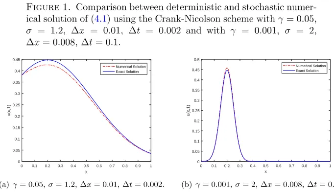
Figure 1. Comparison between deterministic and stochastic numer-ical solution of (4.1) using the Crank-Nicolson scheme withγ= 0.05,
σ = 1.2, ∆x = 0.01, ∆t = 0.002 and with γ = 0.001, σ = 2, ∆x= 0.008, ∆t= 0.1.
0 0.1 0.2 0.3 0.4 0.5 0.6 0.7 0.8 0.9 1
x
0 0.05 0.1 0.15 0.2 0.25 0.3 0.35 0.4 0.45
u(x,1)
Numerical Solution Exact Solution
(a)γ= 0.05,σ= 1.2, ∆x= 0.01, ∆t= 0.002.
0 0.1 0.2 0.3 0.4 0.5 0.6 0.7 0.8 0.9 1 x
0 0.05 0.1 0.15 0.2 0.25 0.3 0.35 0.4 0.45 0.5
u(x,1)
Numerical Solution Exact Solution
(b)γ= 0.001,σ= 2, ∆x= 0.008, ∆t= 0.1.
hence to generate Wiener increments ∆Wnin MATLAB environment of random num-bers the generator, randn(# traj,# step) is used, such that each call to randn(# traj,# step) creates a #traj×#stepmatrix of independentN(0,1) samples.
Example 4.1. Consider the stochastic diffusion equation of the form
ut(x, t) =γuxx(x, t) +σu(x, t) ˙W(t), x∈[0,1], t∈[0,1], (4.1)
with initial condition
u(x,0) = exp (
−(x−0.2)2
γ
)
,
and boundary conditions
u(0, t) = √ 1
4t+ 1exp (
− 0.04
γ(4t+ 1)
)
,
u(1, t) = √ 1
4t+ 1exp (
− 0.64
γ(4t+ 1)
)
.
In absence of the noise term, the exact solution is
u(x, t) =√ 1
4t+ 1exp (
−(x−0.2)2
γ(4t+ 1)
)
.
In this example, in order to qualify numerical results of the considered stochastic diffusion equation, we plot in Figure1the stochastic solution using stochastic Crank-Nicolson scheme (2.6) with γ = 0.05, σ = 1.2, ∆x = 0.01, ∆t = 0.002 and with
of stability of this stochastic implicit method, we have not any restriction for con-sidering the space and time step sizes and refinement of the computational domain does not impose any restriction on the stability scheme. So numerically implicit and unconditional stability of this stochastic method could be used to approximate the solu-tion of stochastic diffusion equasolu-tion. In Table1, some numerical results are presented for solving the stochastic diffusion equation (4.1) using the conditional stable scheme (2.7). The exact deterministic solution and numerical solution of the stochastic
diffu-Table 1. Test white noise SPDE (4.1) by the stochastic scheme (2.7).
N E(u(0.2,1)) E((u(0.2,1))2
5 −1.2703 1.6137 15 0.1389 0.0193 25 0.4101 0.1682 40 0.4498 0.2023 50 0.4961 0.2461 60 0.4639 0.2152
sion equation (4.1) using the stochastic Crank-Nicolson scheme are shown in Figure3
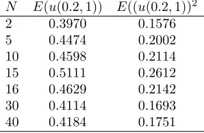
and Figure4on a500×500grid during the time interval[0,1]forγ= 0.001,σ= 0.01 and forγ= 0.002,σ= 0.03, respectively. Also by fix γ= 0.001,σ= 2 andM = 125 the stochastic scheme is convergent withN ≥16. We have shown this in Table3. For
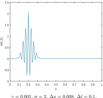
γ = 0.001, σ = 2,∆x= 0.008 and∆t = 0.1, numerical solution (2.7) is shown in Figure2. From the numerical results of this example, we get that the obtained results from the scheme (2.6)quite agreed with the exact one.
Table 2. Test white noise SPDE (4.1) by the stochastic Crank-Nicolson scheme.
γ σ ∆t ∆x E(u(0.2,1)) E((u(0.2,1))2
0.005 1 0.005 0.01 0.4680 0.2190 0.05 1.2 0.02 0.01 0.4353 0.1895 0.001 2 0.04 0.008 0.4736 0.2243 0.01 1.5 0.1 0.01 0.4599 0.2115
Example 4.2. We consider another test example to approximate the solution of stochastic diffusion equation driven by the white noise of the form
ut(x, t) =γuxx(x, t) +σu(x, t) ˙W(t), x∈[0,1], t∈[0,1], (4.2)
with initial condition
u(x,0) = sin(πx), x∈[0,1],
and boundary conditionsu(0, t) =u(1, t) = 0, by use of the stochastic Crank–Nicolson scheme. The problem has an exact solution given by
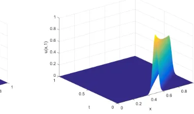
Figure 2. Numerical solution of stochastic advection-diffusion equa-tion by use of the scheme (2.7).
0 0.1 0.2 0.3 0.4 0.5 0.6 0.7 0.8 0.9 1
x
-1 -0.5 0 0.5 1 1.5 2 2.5
u(x,1)
γ= 0.001,σ= 2,∆x= 0.008,∆t= 0.1.
Figure 3. The exact solution and numerical solution of (4.1) using the stochastic Crank-Nicolson method.
(a) The exact solution withγ= 0.001. (b) The numerical solution withγ= 0.001 and
σ= 0.01.
Figure 4. The exact solution and numerical solution of (4.1) using the stochastic Crank-Nicolson method.
(a) The exact solution withγ= 0.002. (b) The numerical solution withγ= 0.002 and
σ= 0.03.
Table 3. Test white noise SPDE (4.1) by the stochastic Crank-Nicolson scheme.
N E(u(0.2,1)) E((u(0.2,1))2
2 0.3970 0.1576 5 0.4474 0.2002 10 0.4598 0.2114 15 0.5111 0.2612 16 0.4629 0.2142 30 0.4114 0.1693 40 0.4184 0.1751
Table 4. Test of white noise SPDE (4.1) by the stochastic scheme (2.7).
N E(u(0.5,1)) E((u(0.5,1))2
5 1.2487 1.5591 10 1.2170 1.4810 15 1.1106 1.2333 30 1.0390 1.0796 40 1.0363 1.0740 45 1.0503 1.1031
see that stability conditions are hold for the scheme (2.7). If we choose γ = 0.001,
σ = 1.5, ∆x= 0.01 and ∆t > 0.04, i.e., N < 25, we will see the scheme (2.7) is
Figure 5. Numerical solution of stochastic advection-diffusion equa-tion using the scheme (2.7).
0 0.1 0.2 0.3 0.4 0.5 0.6 0.7 0.8 0.9 1
x
-80 -60 -40 -20 0 20 40 60 80
u(x,1)
γ= 0.001,σ= 1.5,∆x= 0.01,∆t= 0.1.
Table 5. Test white noise SPDE (4.1) by the stochastic scheme (2.7).
N E(u(0.5,1)) E((u(0.5,1))2
5 1.2487 1.5591 10 1.2170 1.4810 15 1.1106 1.2333 30 1.0390 1.0796 40 1.0363 1.0740 45 1.0503 1.1031
The exact deterministic solution and numerical solution of the stochastic diffusion equation (4.2) using the stochastic Crank–Nicolson scheme have been shown in Figures
8–9on a 500×500grid during the time interval[0,1]forγ= 0.002,σ= 0.03and for
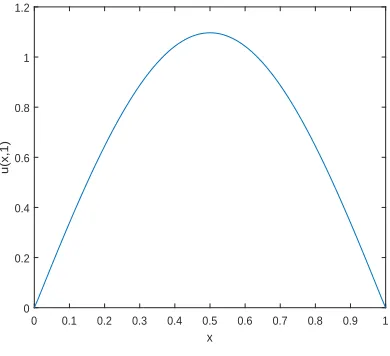
γ= 0.001,σ= 0.001, respectively. Ifγ= 0.001,σ= 1.5 andM = 100, the stochastic scheme is convergent if N ≥ 10. This is obvious from Table 7. Figure 7 shows numerical solution of the scheme (2.7)for valuesγ= 0.001,σ= 1.5,∆x= 0.01 and ∆t= 0.02.
Example 4.3. Consider the following SPDE
ut(x, t) +νux(x, t) =γuxx(x, t) +σu(x, t) ˙W(t), x∈[0,1], t∈[0,1], (4.3)
with the following initial condition
u(x,0) = exp (
−(x−0.5)2
γ
)
Figure 6. Comparison between deterministic and stochastic numer-ical solution of (4.2) using the Crank-Nicolson scheme withγ= 0.002,
σ = 1.8, ∆x = 0.01, ∆t = 0.02 and with γ = 0.001, σ = 1.5, ∆x= 0.01, ∆t= 0.02.
0 0.1 0.2 0.3 0.4 0.5 0.6 0.7 0.8 0.9 1
x
0 0.1 0.2 0.3 0.4 0.5 0.6 0.7 0.8 0.9 1
u(x,1)
Numerical Solution Exact Solution
(a)γ= 0.002,σ= 1.8, ∆x= 0.01, ∆t= 0.02.
0 0.1 0.2 0.3 0.4 0.5 0.6 0.7 0.8 0.9 1
x
0 0.1 0.2 0.3 0.4 0.5 0.6 0.7 0.8 0.9 1
u(x,1)
Numerical Solution Exact Solution
(b)γ= 0.001,σ= 1.5, ∆x= 0.01, ∆t= 0.02.
Figure 7. Numerical solution of stochastic advection-diffusion equa-tion using the scheme (2.7).
0 0.1 0.2 0.3 0.4 0.5 0.6 0.7 0.8 0.9 1
x
0 0.2 0.4 0.6 0.8 1 1.2
u(x,1)
γ= 0.001,σ= 1.5, ∆x= 0.01,∆t= 0.02.
with the boundary conditions
u(0, t) = √ 1
4t+ 1exp (
−(−0.5−νt)2
γ(4t+ 1)
)
,
u(1, t) = √ 1
4t+ 1exp (
−(0.5−νt)2
γ(4t+ 1)
)
Table 6. Test of white noise SPDE (4.2) by the stochastic Crank-Nicolson scheme.
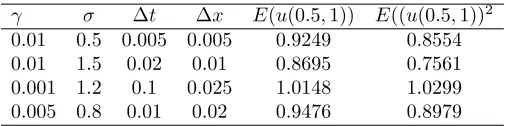
γ σ ∆t ∆x E(u(0.5,1)) E((u(0.5,1))2
0.01 0.5 0.005 0.005 0.9249 0.8554 0.01 1.5 0.02 0.01 0.8695 0.7561 0.001 1.2 0.1 0.025 1.0148 1.0299 0.005 0.8 0.01 0.02 0.9476 0.8979
Figure 8. Exact solution and numerical solution of (4.2) using sto-chastic Crank-Nicolson scheme.
(a) The exact solution withγ= 0.002. (b) The numerical solution withγ= 0.002 and
σ= 0.03.
Figure 9. Exact solution and numerical solution of (4.2) using sto-chastic Crank-Nicolson scheme.
(a) The exact solution withγ= 0.001. (b) The numerical solution withγ= 0.001 and
σ= 0.001.
It is easy to verify that in the absence of the noise term, the exact solution is
u(x, t) =√ 1
4t+ 1exp (
−(x−0.5−νt)2
γ(4t+ 1)
)
Table 7. Test of white noise SPDE (4.2) by the stochastic Crank-Nicolson scheme.
N E(u(0.5,1)) E((u(0.5,1))2
2 0.9421 0.8876 5 0.9998 0.9997 10 1.0192 1.0387 15 1.0525 1.1077 20 1.1183 1.2507 40 1.0152 1.0307 100 1.1005 1.2111
Table 8. Test of white noise SPDE (4.3) by stochastic scheme (2.7).
N E(u(0.6,1)) E((u(0.6,1))2
80 −2.6964E+ 20 7.2704E+ 40 90 −1.2982E+ 19 1.6853E+ 38 100 −8.4556E+ 16 7.1497E+ 33 150 0.1114 0.0124 152 0.1162 0.0135 200 0.1068 0.0114
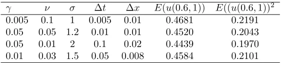
Table 9. Test white noise SPDE (4.3) by the stochastic Crank-Nicolson scheme.
γ ν σ ∆t ∆x E(u(0.6,1)) E((u(0.6,1))2
0.005 0.1 1 0.005 0.01 0.4681 0.2191 0.05 0.05 1.2 0.01 0.01 0.4520 0.2043 0.05 0.01 2 0.1 0.02 0.4439 0.1970 0.01 0.03 1.5 0.05 0.008 0.4584 0.2101
Table 10. Test white noise SPDE (4.3) by the stochastic Crank-Nicolson scheme.
N E(u(0.6,1)) E((u(0.6,1))2
2 0.3882 0.1507 5 0.3236 0.1047 10 0.4339 0.1882 20 0.3343 0.1117 40 0.3900 0.1521 150 0.3910 0.1529 200 0.3940 0.1552
Figure 10. Comparison between deterministic and stochastic nu-merical solutions of (4.3) using the Crank-Nicolson scheme with
γ = 0.01, ν = 0.01, σ = 2.5, ∆x = 0.01 and ∆t = 0.001 and with
γ= 0.001,ν = 0.02,σ=−2, ∆x= 0.004 and ∆t= 0.01.
0 0.1 0.2 0.3 0.4 0.5 0.6 0.7 0.8 0.9 1
x
0 0.05 0.1 0.15 0.2 0.25 0.3 0.35 0.4 0.45 0.5
u(x,1)
Numerical Solution Exact Solution
(a) γ= 0.01, ν = 0.01, σ = 2.5, ∆x = 0.01, ∆t= 0.001.
0 0.1 0.2 0.3 0.4 0.5 0.6 0.7 0.8 0.9 1
x
0 0.05 0.1 0.15 0.2 0.25 0.3 0.35 0.4 0.45
u(x,1)
Numerical Solution Exact Solution
(b)γ= 0.001,ν= 0.02,σ=−2, ∆x= 0.004, ∆t= 0.01.
Figure 11. Numerical solution of stochastic advection diffusion equation using the scheme (2.7).
0 0.1 0.2 0.3 0.4 0.5 0.6 0.7 0.8 0.9 1
x
-2 -1.5 -1 -0.5 0 0.5 1 1.5 2
u(x,1)
1018
γ= 0.001,ν= 0.02,σ=−2, ∆x= 0.004, ∆t= 0.01.
ν = 0.01, σ = 2.5, ∆x= 0.01, ∆t = 0.001 and for γ = 0.001, ν = 0.02, σ = −2, ∆x= 0.004,∆t= 0.01.
Figure 12. Exact solution and numerical solution of (4.3) using the stochastic Crank-Nicolson scheme.
(a) Exact solution withγ= 0.002 andν= 1.2. (b) The numerical solution withγ= 0.002,ν= 1.2 andσ= 0.01.
Figure 13. Exact solution and numerical solution of (4.3) using the stochastic Crank-Nicolson scheme.
(a) The exact solution withγ= 0.001 andν= 1.
(b) The numerical solution withγ= 0.001,ν= 1 andσ= 0.01.
The computational results for approximating the solution of SPDE (4.3) are shown in Table9 by consideration several values for time step and space size, ν, γ and σ. In Figures12–13we have shown the exact deterministic solution and the approxima-tion of the stochastic advecapproxima-tion diffusion equaapproxima-tion using the stochastic Crank-Nicolson scheme on a500×500 grid withγ= 0.002,ν= 1.2, σ= 0.01 andγ= 0.001,ν= 1,
σ= 0.01during the time interval [0,1]. If we chooseγ= 0.01,ν = 0.1,σ=−2 and
5. Conclusion
In this paper, a stochastic finite difference scheme has been applied for the solution of stochastic advection-diffusion equation. Also, we have provided analysis of consis-tency, stability, and convergence of the stochastic difference scheme. The scheme has applied to three problems have given in the paper, each with different boundary con-ditions and has given an initial condition. The numerical results have obtained by the stochastic difference scheme is compared with the exact solution and the scheme in [7], to verify the accuracy and efficiency of the stochastic difference scheme.
References
[1] E. J. Allen , S. J. Novose, and Z. C. Zhang,Finite element and difference approximation of some linear stochastic partial differential equations, Stochastic Rep.,64(1998), 117–142. [2] M. Bishehniasar and A. R. Soheili, Approximation of stochastic advection-diffusion equation
using compact finite difference technique, Iranian Journal of Science & Technology, 37(A3) (2013), 327–333.
[3] I. Gyongy and C. Rovira,OnLp–solution of semilinear stochastic partial differential equation,
Stoch. Proc. Appl.,90(2000), 83–108.
[4] I. Gyongy,Existence and uniqueness results for semilinear stochastic partial differential, Stoch. Proc. Appl.,73(1998), 271–299.
[5] M. Kamrani and S. M. Hosseini,The role of the coefficients of a general SPDE on the stability and convergence of the finite difference method, J. Comput. Appl. Math.,234(2010), 1426–1434. [6] P. E. Kloeden and E. Platen,Numerical solution of stochastic differential equations, Springer
Berlin, 1995.
[7] M. Namjoo and A. Mohebbian,Approximation of stochastic advection-diffusion equations with finite difference scheme, Journal of Mathematical Modeling,4(2016), 1–18.
[8] G. D. Prato and L. Tubaro,Stochastic partial differential equations and application, Longman scientific and technical, Harlow, 1992.
[9] C. Roth,Difference methods for stochastic partial differential equations, Z. Zngew. Math. Mech.,
82(2002), 821–830.
[10] A. R. Soheili, M. B. Niasar, and M. Arezoomandan, Approximation of stochastic parabolic differential equations with two different finite difference schemes, Bulletin of the Iranian Math-ematical Society,37(2011), 61–83.
[11] J. C. Strikwerda,Finite difference schemes and partial differential equations, 2nd ed. Society for Industrial and Applied Mathematics, Philadelphia, 2004.